To lockdown? When to peak? Will there be an end? A macroeconomic analysis on COVID-19 epidemic in the United States

Abstract

In this paper, we construct an extended SIR model with agents optimally choosing outdoor activities. We calibrate the model and match it to the data from the United States. The model predicts the epidemic in the United States very well. Without government intervention, our simulation shows that the epidemic peaks on 22 March, 2020 and ends on 29 August, 2022. By the end of the epidemic, more than 21 million people will be infected, and the death toll is close to 3.8 million. We further conduct counterfactual experiments to evaluate the effectiveness of different polices against this pandemic. We find that no single policy can effectively suppress the epidemic, and the most effective policy is a hybrid policy with lockdown and broadening testing. Lockdown policy alone is ineffective in controlling the epidemic as agents would have optimally stayed at home anyway if the infection risk is high even without a lockdown. Broadening testing solely will accelerate the return to normal life as there are fewer infected people hanging around. However, as people do not internalize the social costs of returning to normal life, the epidemic could get even worse. Increasing medical capacity without any other measures only has temporary effects on reducing the death toll. We also find that random testing is too inefficient unless a majority of population is infected.

1. Introduction

Life is no longer the same for an American since the first case of COVID-19 recorded on 22 January, 2020. The confirmed cases have skyrocketed with more than a million American tested positive and tens of thousands of lives being taken away in about three months. States after states have issued the state of emergency order. Following the footsteps of many Asian and European countries, cities are locked down to tackle the virus. With such a strong measure on limiting the freedom of people, a question naturally arises: Is the measure effective and necessary?

One challenge for tackling COVID-19 is the high proportion of no symptoms or mild cases (or long incubation periods) which could continue spreading the virus. Broadening testing will keep people informed with their truth health status. This works together with an effective quarantine order could effectively lower the unaware infected people hanging around in the community and slowdown the spread. The strategy has been used by many countries without a lockdown.

The COVID-19 has already become a pandemic, but countries around the world are posing substantially different death rates. The case fatality rates vary from more than 10% in Italy and the United Kingdom to less than 1% in Singapore. The number is about 6% in the United States as of 8 May, 2020. One possible explanation to the large discrepancies in death rates is the collapse of healthcare systems in many countries. Increasing medical capacities, such as building temporary hospitals and producing emergency ventilators, are particularly important in lowering the death rates. The overall effect of medical capacity to the epidemic is another issue worth studying.

In this paper, we construct an extended SIR model and match the model to the available data in the United States. We simulate the benchmark model under the situation of no government intervention. By 29 August, 2022, more than 21 million of people will be infected in the whole epidemic and the death toll is close to 3.8 million. We then perform experiments to investigate the effects of different policies against the epidemic, including lockdown, broadening testing, increasing medical capacity and a hybrid policy combining lockdown and broadening testing. We find that no policies alone can successfully tackle the epidemic. Locking down only results in delaying the peak and the end of the epidemic because a second wave of infection will quickly emerge after reopening. Broadening testing solely lowers the risk of infection because fewer infected individuals are hanging around. However, people do not internalize the social costs of spreading the virus, and will choose to return to normal life too soon, leading to a worsened epidemic. Increasing medical capacity alone lowers the costs of infection initially. However, similar to broadening testing, more people will hang around, and the resulted increases in infection and medical demand will erase the gain of an enlarged medical capacity. In the end, we experiment on a combination of policies with lockdown and broadening testing and find that such policy successfully limits the spread of the virus. This is because when people do not internalize the social costs of spreading the virus, lockdown can effectively prevent unconfirmed infected cases from returning to normal life and spreading the virus further. Our simulation shows that the hybrid policy stops the epidemic completely.

As the pandemic of COVID-19 is still ongoing, the literature is rapidly growing. This paper is closely related to papers using a standard SIR model to study COVID-19. For example, Alvarez et al. (2020) study the optimal lockdown policy. Eichenbaum et al. (2020) extend the standard SIR model to study the economic interactions with the spread of virus. Garibaldi et al. (2020) focus on the matching mechanism in the SIR model. Berger et al. (2020) extend an SIR model to SEIR in order to study the effect of testing and quarantine. Other papers include Krueger et al. (2020), Aum et al. (2020), Toda (2020), Favero (2020), Gonzalez-Eiras and Niepelt (2020), Bethune and Korinek (2020). Lockdowns around the world also raises lots of research interests in working from home and people being affected by the stay-at-home order. Dingel and Neiman (2020) estimate that 34% of US jobs can be performed at home. Using American Time Use Survey, Alon et al. (2020) analyze the sectors and groups of people that are most affected by the stay-at-home order. Other works examining different countries include Saltiel (2020), Gottlieb et al. (2020), Delaporte and Pena (2020).

2. Model

2.1. Agent

Consider an infinite-horizon model with a continuum of agents. In each period, all agents are endowed with one unit of time and allocating their time to working away from home l, working from home l^h, and outdoor consumption c^o. Agents receive utility from two consumption goods - indoor consumption cⁱ and outdoor consumption c^o. Let $u(c_t^i,c_t^o)$ be the period utility at time t. The budget constraint and time constraint at time t are given respectively by

$$\begin{array}{cc}& c_t^i=w_t{l}_t+w_t^h{l}_t^h+{\tau }_t\hfill \\ & c_t^o+l_t+l_t^h=1\hfill \end{array}$$

where w_t and $w_t^h$ are the wages for working away from home and working from home, respectively. τ_t is a direct transfer. Hence, outdoor consumption costs time while indoor consumption is bought from the market.

We extend the SIR model and assume that there are five possible states: susceptible, infected, confirmed with mild symptoms, confirmed with severe symptoms, and recovered.

2.1.1. Susceptible

Agents are healthy in the susceptible state and choose cⁱ, c^o, l, l^h to maximize their lifetime utility. However, outdoor consumption and working away from home could lead to infectious exposures. Assume that an agent has a probability p(c^o, l, η) of being infected, where η is the proportion of infected people among people who are hanging around by choosing c^o > 0 or l > 0. If an agent is infected by the virus, he will enter the infected state.

2.1.2. Infected

In the infected state, an agent acts like a susceptible agent. This could be interpreted as the incubation period, the misinterpretation of a common cold or the waiting time for the test results. The agent in this phase is assumed to be unaware of being infected and will share the same decision rules as a healthy agent. However, with a probability ψ, the agent will be tested positive with the disease and become a confirmed case. A confirmed case has probabilities λ to have mild symptoms and $1-\lambda$ to have severe symptoms. With a probability γ, the infected agent will recover without being tested positive.

2.1.3. Confirmed with mild symptoms or severe symptoms

For confirmed cases with either mild or severe symptoms, working ($l=l^h=0$) or hanging around (c^o) are prohibited, and hence the agents are effectively quarantined. For mild cases, agents will recover with a probability of γ in each period. For severe cases, there is a probability γ_s (γ_s < γ) of recovery and a probability π(MD) of death, where MD is the medical demand. If the medical demand increases relative to the capacity of the health care system, mortality rate increases. Hence, we assume π′(MD) > 0.

2.1.4. Recover

This state includes agents who are recovered from the states of infected, confirmed with mild symptoms and confirmed with severe symptoms. In this state, agent is immune to infection with the same virus. However, since little has been known for the nature of COVID-19 regarding whether an agent will be infected again, we assume that there is a probability ζ that an agent will be in the susceptible state again.

2.2. Production technology

The production takes both types of labor as inputs, l and l^h. We assume that the marginal product of labor is always larger for working away from home, i.e. $\frac{dY}{dL}>\frac{dY}{d{L}^h},$ where Y, L, L^h are the aggregate output, the labor away and the labor at home respectively. As a result, a worker will always choose to commute to work if there are no risks of being infected. To be specific, we assume

$$Y=A(L^h+L)+B{L}^{\alpha }.$$

Hence, $w_t^h=A$ and $w_t=A+\alpha B{L}_t^{\alpha -1}$ in equilibrium. Profit is being allocated evenly in the population every period through the direct transfer τ_t.

2.3. Demographic evolution

We will specify the transition of states in this section. Assume that $X_t^s,$ $X_t^i,$ $X_t^m,$ $X_t^s,$ $X_t^r$ and $X_t^d$ be the total number of agents in state of susceptible, infected, confirmed with mild symptoms, confirmed with severe symptoms, recovered and death at time t respectively. The evolutions are given by

$$\begin{array}{cc}\hfill X_{t+1}^i& =p(c_t^o,l_t,{\eta }_t)X_t^s+(1-\psi -\gamma )X_t^i,\hfill \\ \hfill X_{t+1}^m& =\psi \lambda X_t^i+(1-\gamma )X_t^m,\hfill \\ \hfill X_{t+1}^s& =\psi (1-\lambda )X_t^i+(1-{\gamma }_s-\pi \left(M{D}_t\right))X_t^s,\hfill \\ \hfill X_{t+1}^r& =\gamma X_t^i+\gamma X_t^m+{\gamma }_s{X}_t^s+(1-\zeta )X_t^r,\hfill \\ \hfill X_{t+1}^s& =\zeta X_t^r+(1-p(c_t^o,l_t,{\eta }_t))X_t^s,\hfill \\ \hfill X_{t+1}^d& =\pi \left(M{D}_t\right)X_t^s+X_t^d.\hfill \end{array}$$

Also, the infected hangout ratio η_t is given by

$${\eta }_t=\frac{X_t^i}{X_t^s+X_t^i+X_t^r}.$$

Since all the confirmed cases are being prohibited from hanging around until they are recovered, the virus is spread mainly through those unaware infected agents.

2.4. Dynamic program

Let U be the value function of a susceptible agent, and let V be the value function of an infected agent. The value of being a susceptible agent is given by

$$U_t=\max \{u(c_t^i,c_t^o)+\beta [(1-p(c_t^o,l_t,{\eta }_t\left)\right)U_{t+1}+p(c_t^o,l_t,{\eta }_t)V_{t+1}]\}$$

subject to

$$\begin{array}{cc}& c_t^i=w_t{l}_t+w_t^h{l}_t^h+{\tau }_t,\hfill \\ & c_t^o+l_t+l_t^h=1,\hfill \\ & c_t^o\le {\overline{c}}_t^o,\hfill \\ & l_t\le {\overline{l}}_t,\hfill \end{array}$$

where β is the discount factor, and ${\overline{c}}_t^o$ and ${\overline{l}}_t$ are the exogenous lockdown parameters. Without lockdowns, ${\overline{c}}_t^o={\overline{l}}_t=1$. Let $c_t^{i*},$ $c_t^{o*},$ $l_t^{*},$ $l_t^{h*}$ be the solution in the above maximization.

Since the agent is unaware of being infected, the decision rule is the same as a susceptible agent. The value of being an infected agent is given by

$$V_t=u(c_t^{i*},c_t^{o*})+\beta [\psi W_{t+1}+\gamma R_{t+1}+(1-\psi -\gamma )V_{t+1}]$$

where W is the value function of being tested positive with the disease and R is the value for agents who have recovered from the disease.

For agents who are diagnosed with the disease, let W^m and W^s be the value functions for having mild and severe symptoms respectively. We have

$$\begin{array}{cc}\hfill W_t& =\lambda W_t^m+(1-\lambda )W_t^s,\hfill \\ \hfill W_t^m& =u({\tau }_t,0)+\beta [\gamma R_{t+1}+(1-\gamma )W_{t+1}^m],\hfill \\ \hfill W_t^s& =u({\tau }_t,0)+\beta [\pi \left(M{D}_t\right)v_d+{\gamma }_s{R}_{t+1}+(1-{\gamma }_s-\pi \left(M{D}_t\right))W_{t+1}^s],\hfill \end{array}$$

where v_d is the value of death, which we will normalize to 0. As agents are restricted from working or outdoor consumption after being tested positive, they can only consume the transfer received until they are recovered because there is no saving in the model.

Finally, let R be the value of recovered agent and is given by

$$R_t=u(c_t^{i*},c_t^{o*})+\beta [\zeta U_{t+1}+(1-\zeta )R_{t+1}]$$

Again, agents are unsure whether he is susceptible to the disease or not, and lots of people might not even realize that they have caught the disease as people recover from the disease before they are tested. We therefore assume that agents in this state follow the decision rule of that for a susceptible agent as well.

3. Calibration

In this section, we calibrate the model to match the pandemic of COVID-19 in the United States. We first divide the parameters into different categories and discuss the setting of the functional forms used. We then describe the data moments used in the calibration.

3.1. Parameters

3.1.1. Preference

One model period is assumed to be one day. The discount factor β is set as 0.96^1/365. Assume that the period utility is given by a standard CES utility

$$u(c^i,c^o)=\frac{c^{i1-\varphi }}{1-\varphi }+\mu \frac{c^{o1-\varphi }}{1-\varphi }$$

Although the intertemporal marginal rate of substitution tends to be small in the macroeconomic literature, we set $\varphi =0.5$ as the model period is only one day. The substitutability of consumption between today and tomorrow should be much higher than the consumption between today and next year when the model period is one year. The remaining parameter left to be calibrated is μ.

3.1.2. Labor market

The three parameters related to the labor market are A, B and α in the production function. Without loss of generality, we normalize $A=1$. Also, we set $\alpha =0.7$ as that for a standard Cobb-Douglas production function.2 Since there exist universal transfers in the model, we manage to match the transfers with the benefits observed in the data. According to the United States Department of Labor, the average weekly benefit in the second quarter of 2019 is $366.53 while the average weekly wage in the same period is $1106. Hence, we set $\tau /wl=0.3314$. We further normalize the total initial population to one and target $l=0.5,$ as discussed in the next section, we have $B=0.9005$.

3.1.3. Lockdown

The lockdown parameters ${\overline{c}}^o$ and $\overline{l}$ are the parameters that we will experiment with. The default value is one, representing that there are no restrictions in outdoor consumption and working away from home.

3.1.4. Contagious parameters

In the model, p(c^o, l, η) governs how the virus is being transmitted. We specify the functional form as:

$$p(c^o,l,\eta )=\chi ((1-\nu )c^o+\nu l){\eta }^{\kappa }.$$

Under this specification, ${\lim }_{\eta \to 0}p=0$ and the infection probability goes to zero when no infected agents are hanging around. ν is the relative exposure parameter between working away from home and outdoor consumption. Eichenbaum et al. (2020) estimate that 16% of transmissions are related to consumption while 17% of transmissions are related to work. Consistent with their findings, we set $\nu =0.5,$ representing equal probability of exposure in the benchmark. A sensitivity test will be provided in the next section. The remaining two parameters χ and κ will be calibrated by matching the United States spreading data.

3.1.5. Disease

Finally, the parameters affecting the severity and the number of cases of the disease include ψ, λ, γ, γ_s and ζ. We also need to specify the mortality π(MD). According to Guan (2020), the incubation period has a median of four days. We assume that it takes an extra two days between the appearing of the first symptom and the time of being tested positive and set $\psi =0.11$.3 According to Wu and McGoogan (2020), about 81% of 44,415 confirmed cases show mild symptoms, 14% show severe symptoms and 5% are critical. Hence, we set $\lambda =0.81$. For the mortality function, we assume that

$$\begin{array}{cc}\hfill \pi \left(MD\right)& =\delta +(1-\delta -{\gamma }_s)(1-e^{-\frac{MD}{\omega }}),\hfill \\ \hfill MD& =\theta X^m+(1-\theta )X^s,\hfill \end{array}$$

where δ is the basic fatality rate of the disease. The death rate will increase if medical demand, MD, increases relative to the capacity of the health care system, ω. We interpret ω as the medical capacity of the health care system which includes available physicians, intensive care beds, ventilators, and etc. We assume medical demand MD to be a weighted average of mild and severe cases with a weight of θ < 0.5 for mild cases. Since the epidemic is still on going, the recovery and fatality statistics are very likely to be biased at this point. Therefore, it is better to leave these parameters to be calibrated by matching the observed data moments. Finally, as mentioned in the previous section, ζ is a parameter we will experiment on. We set ζ at zero in the benchmark. That is, in the benchmark model, once people have caught the disease, they are immune from the disease forever.

In all, there are eight parameters remained to be calibrated, including μ, χ, κ, γ, γ_s, θ, δ and ω.

3.2. Moments

We focus on matching the observed confirmed cases, deaths, and cases of recovery since the first case was recorded in the United States.4 Also, as there are no lockdowns in the benchmark model, it is more suitable to fit the observed trend before the implementation of any lockdown measures within the United States. To this end, the calibration periods ranges from 22 January, 2020 when the first case was recorded to 18 March, 2020 when California announced the first mandatory stay-at-home order on 19 March, 2020.5 We also set the labor hours at 0.5 before the epidemic starts. This number suggests that individuals spend half of the non-sleeping hours on working and the other half on outdoor leisure.

4. Simulation

Although it is a more common practice to simulate the decision rules under rational expectation, people could hardly foresee the future under such a rapid changing environment, including the virus spreading and the sudden policy changes. We thus simulate the time path by assuming that agents make decisions based on what they observe today and stay at the current level. The simulation starts at a steady state of no infection. We then randomly let one individual be infected, and the virus starts to spread in the economy from that point on. We define the period to be 22 January, 2020 when there is exactly one case (or more than one cases) being confirmed with COVID-19.6 We report in Table 1 the 8 parameters that are used to match the observed trend in the data before 19 March, 2020.

Table 1.

Parameter values.

Parameters	Value
μ	1.2231
κ	1.1022
χ	3.2418
γ	0.005043
γs	0.002011
θ	0.2108
δ	0.02100
ω	0.0001753

At the first glance, the recovery probabilities γ and γ_s are low while the death probability is high compared to other studies. Atkeson (2020) and Alvarez et al. (2020) both follow Wang (2020) to use a recover probability of 1/18. However, we doubt that the number is highly biased upward.7 Also, as the United States recorded only 105 cases of recovery from 7783 confirmed cases on 18 March, 2020, it is not surprising that γ and γ_s are so small. As for the death rate, a daily mortality rate of 2.1% is high. However, recall that only agents with severe symptoms die. The true mortality rate is thus much lower as there are only 19% out of the confirmed cases with severe symptoms. Moreover, lots of agents recovered directly without being tested.

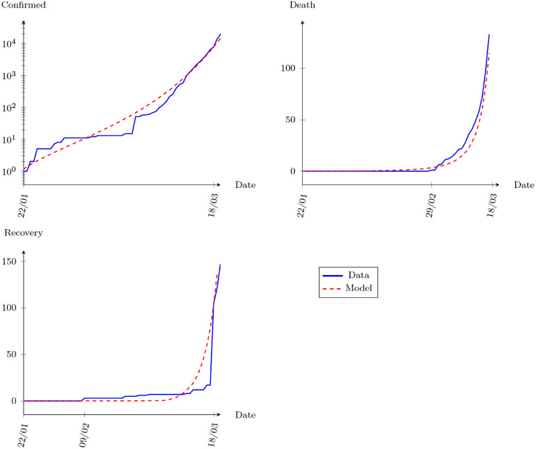
We plot in Fig. 1 the calibration results with three panels exhibiting the simulated confirmed cases, death tolls and recovery cases respectively.8 The blue line shows the observed data while the red line shows the model prediction. The model matches the United States experiences before 19 March, 2020 very well. We now proceed to model predictions based on the benchmark calibration from 19 March, 2020 onwards.

Fig. 1.

Calibration Results: Model vs Data, 22 January, 2020 to 18 March, 2020.

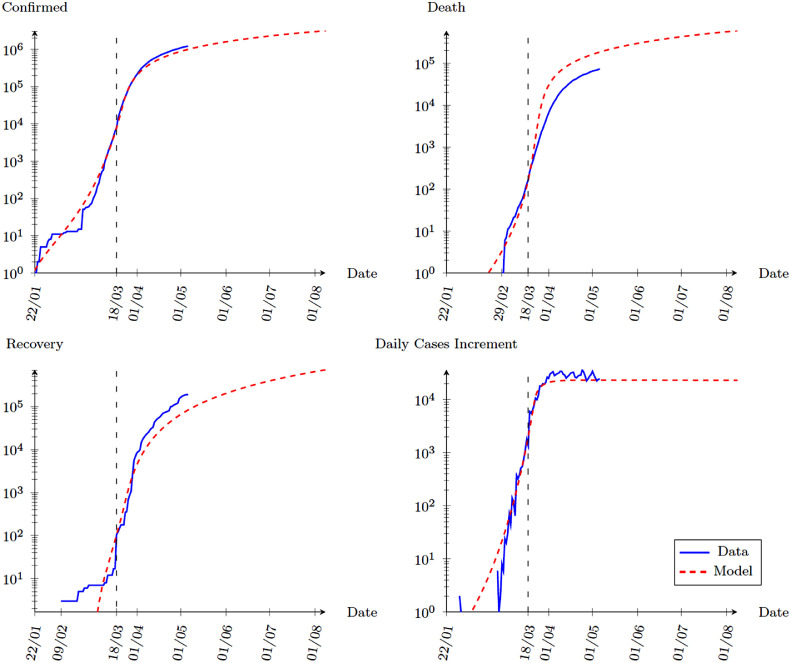
The total number of confirmed cases of COVID-19 has surged since 18 March, 2020. More than 1.2 million cases were recorded as of 6 May, 2020. The death toll has also raised above 70 thousand. Without any government intervention, our model predicts similar severity of the epidemic. Fig. 2 shows our simulation results for 200 days since 22 January, 2020, that is, 8 August, 2020. Observing the top-left panel, the model predicts the confirmed cases very well, especially the slow down after April. The model slightly underestimates the severity of the epidemic. However, it successfully predicts that the spread of the virus has become more stable after April. For the death toll and total recovery, the model overestimates the death rates while underestimates the recovery rates. This is not surprising as the calibration target is the trend when COVID-19 first spread. Lots of research has been done on the virus since then and we can expect the recovery rates to go up and the death rates to go down as we are more capable of tackling the virus.

Fig. 2.

Benchmark Simulation: Model vs Data, 22 January to 8 August, 2020.

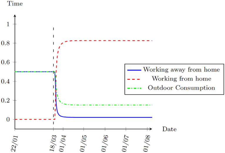
One interesting fact is that the benchmark simulation assumes no government interventions. Without any lockdown, the model suggests that the virus spread will be more stable after April. The reason is that in view of the risks of being infected, people are optimally reducing outdoor consumption and the working time away from home. Fig. 3 shows the decisions for time use. The model suggests that the risks of infection are severe enough to give people incentives to work from home since 21 March, 2020.

Fig. 3.

Benchmark Simulation: Time Allocation, 22 January to 8 August, 2020.

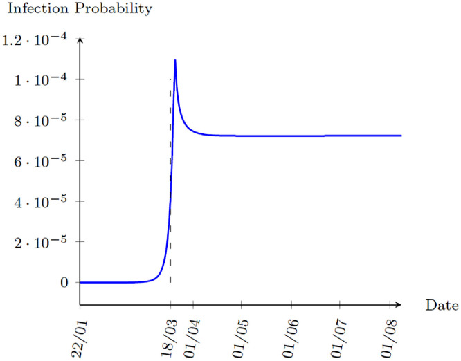
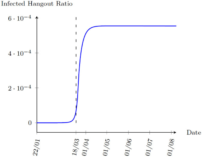
Finally, Fig. 4 plots the infection probability in each day. The model shows that the infection probability peaks on 21 March, 2020 and starts to decrease as people rapidly reduce outdoor consumption and start to work from home. Another interesting statistic is the infected hangout ratio, η_t. In the model, when an agent is tested positive for COVID-19, they are quarantined. Hence, the infected agents hanging around are those who are unaware of the fact that they are infected. Fig. 5 shows the simulated infected hangout ratio. Both statistics suggest that the speed of the virus spread is growing rapidly during late March until people decide to stay home to avoid the risk of being infected. The spread of the virus is stabilized since then.

Fig. 4.

Benchmark Simulation: Infection Probability, 22 January to 8 August, 2020.

Fig. 5.

Benchmark Simulation: Infected Hangout Ratio, 22 January to 8 August, 2020.

5. Counterfactual experiments

In this section, we are interested in three policy experiments. First, we would like to study how effective lockdown is on limiting the spread of the virus. Second, the main channel of transmission of the virus is the unaware infected people with very mild or no symptoms. Broadening testing and quarantining confirmed cases as soon as possible is a way of tackling the epidemic. We thus would like to investigate the effectiveness of policies related to testing. Third, as one suggested reason of the high fatality rate of COVID-19 is the collapsed of health care system, we would like to know if increasing medical capacity could lower the death toll.

To compare the effects of different policies, we define a peak of an epidemic as the point with the largest increment of infections and the end of an epidemic as the total number of infected population has reached its peak under non-binding policy restrictions.9 We will compare the timing of peak and the end of the epidemic, the number of infected cases, and death toll at the end of the epidemic under different policies. We will also compare a normal life index (NLI), constructed by $l+c^o,$ to evaluate how much people are returning to their pre-epidemic life. In the benchmark simulation, the peak of the epidemic is on 22 March, 2020 and the end of the epidemic is on 29 August, 2022. Total infection cases exceed 21 million and the death toll is closed to 3.8 million. The normal life index is 0.181 in the end of the epidemic.

5.1. Lockdown

The first experiment is to examine the effect of a lockdown. From the benchmark simulation, it is obvious that a partial lockdown ($\overline{l}>0$ or $\overline{c}>0$) would be ineffective as people are optimally reducing their consumption on outdoor activities and switching to work from home. Here, we will examine three dimensions of possible lockdown: (1) the duration of lockdown, (2) the selective lockdown and (3) the reopening scheme.

5.1.1. Duration of lockdown

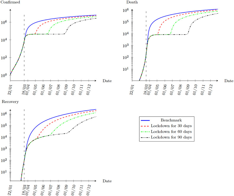
In this part, we study the effects of different lengths of lockdown. Assume that the government decides a complete lockdown ($\overline{l}={\overline{c}}^o=0$) on 19 March, 2020. Fig. 6 shows the effects of a lockdown of 30 days, 60 days and 90 days. In all cases, locking down simply delays the epidemic. Once the restriction is lifted, a second wave of virus starts to spread. This fact is more clear when we compare the effects of different policies in Table 2 .

Fig. 6.

Simulation with different lengths of lockdown, 22 January to 31 December, 2020.

Table 2.

Summary - lockdown.

	Peak	End	Infection (End)	Death Toll (End)	NLI (End)
Benchmark	22-Mar-20	29-Aug-22	21,171,782	3,797,870	0.181
Lockdown 30 days	4-May-20	10-Oct-22	21,199,163	3,802,764	0.181
Lockdown 60 days	23-Jun-20	29-Nov-22	21,188,555	3,800,828	0.181
Lockdown 90 days	31-Aug-20	7-Feb-23	21,204,736	3,803,754	0.181
Lockdown co	22-Mar-20	29-Aug-22	21,168,294	3,797,236	0.181
Lockdown l	19-Apr-20	7-Sep-22	21,197,699	3,802,546	0.181
Phased Reopening	3-May-20	10-Oct-22	21,193,463	3,801,729	0.181
Gradual Reopening	23-May-20	29-Oct-22	21,200,929	3,803,069	0.181
Endogenous Reopening	26-Jul-20	22-Dec-22	21,207,973	3,804,302	0.181

5.1.2. Selective lockdown

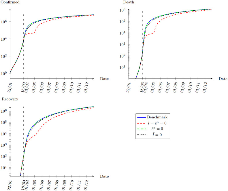
Fig. 7 compares the effects of locking down both outdoor consumption and working away from home, locking only outdoor consumption, and locking only working away from home for 30 days. As expected, the effect is very small if we do not shutdown both outdoor consumption and working away from home.

Fig. 7.

Simulation with selective lockdown, 22 January to 31 December, 2020.

5.1.3. Reopening scheme

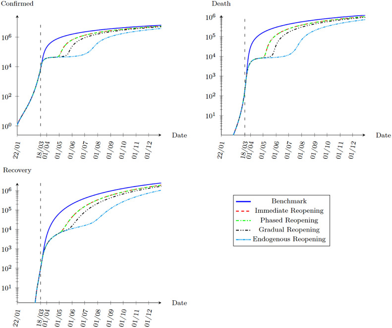
Finally, we would like to know the effects of different reopening policies. We consider four possible schemes. First, we examine an immediate reopening with all restrictions lifted. Second, we consider a phased reopening by relaxing the labor supply restrictions first and extending the outdoor consumption restrictions for another 30 days. Third, we consider a gradual reopening scheme with the lockdown parameters $\overline{l}$ and ${\overline{c}}^o$ increasing by 0.25 for every 30 days. Finally, we consider an endogenous reopening scheme where we assume that $\overline{l}$ and ${\overline{c}}^o$ increase by 0.1 if the number of newly confirmed cases decreases for 7 consecutive days. The results are shown in Fig. 8 .

Fig. 8.

Simulation with different Reopening Schemes after Lockdown, 22 January to 31 December, 2020.

5.1.4. Short summary

Overall speaking, the effect of lockdown is to delay the epidemic. Table 2 shows the results of all lockdown experiments. Comparing with the benchmark simulation, all the lockdown experiments point that temporary lockdown will only delay the spread of the virus. The spread of the virus will quickly catch up once the lockdown is over. The reason is simple. If there are infected agents hang around after the lockdown, it will create another wave of spreading. In all cases, the economy will arrive at the same long run equilibrium when people optimally perform social distancing with the normal life index stays at 0.181.

5.2. Broadening testing

As mentioned before, the main channel of transmission of the COVID-19 virus is from unaware infected people with no or mild symptoms. In this section, we provide experiments on policies of broadening testing which aim at reducing the number of infected individuals hanging around. We consider two possible policies: (1) rapid and target testing, and (2) random testing.

5.2.1. Rapid testing and target testing

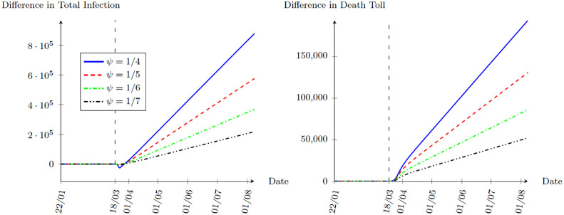
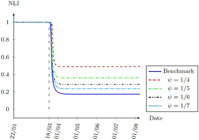
Developing rapid testing and improving identification for high-risk individuals could limit the length in the unaware infected stage. For example, immediate testing on other family members when a family member is confirmed even they are showing no symptoms can effectively lower the risk of community transmissions by identifying potential cases earlier. In the model, the policy goal is to shorten the length of the infected state. In the benchmark calibration, the median of switching from infected state to confirmed state is assumed to be 6 days, which is about 9 days on average. We will experiment ψ with an average duration in the infected state between 4 days to 7 days, that is $\psi =\{1/4,1/5,1/6,1/7\}$. Fig. 9 plots the differences in total infection and death toll relative to the benchmark. Interestingly, although a larger ψ initially reduces the total infection, the situation gets worse as time goes by with both total infection and death toll rise above the benchmark level. When we look at the NLI as shown in Fig. 10 , people are moving closer to the normal life. As rapid and target testing permanently lower the risk of exposure to the virus, people optimally increase outdoor consumption and return to normal workplace. However, people do not internalize the probability of spreading the virus. As a result, increases in ψ worsen the long run epidemic equilibrium while people enjoy normal life more.

Fig. 9.

Simulation with different ψ, 22 January to 31 December, 2020.

Fig. 10.

Normal Life Index ($l+c^o$) under different ψ, 22 January to 31 December, 2020.

5.2.2. Random testing

Many countries have started to expand the scope of testing by randomly sample residents for COVID-19 testing. The result could be informative for policy makers to know the severity of the epidemic. In this section, we study the effects of such a policy. Suppose in the beginning of each period, M people who are not in the confirmed state are randomly drawn for testing. An agent in the infected state, if selected, will receive a positive test result and immediately move to the confirmed state. As of 22 May, 2020, the United States has more than 13 million tests reported and the daily test number is close to 400 thousand. The average number of tests between 19 March to 22 May, 2020 is about 200 thousand. We experiment $M=200,000$ and a 10 times expansion of random testing, $M=2,000,000$. The results are very close to the benchmark with the NLI increasing slightly to 0.191 under $M=2,000,000$. Essentially, random testing is too inefficient unless a majority of population is infected. It thus remains a tool for policy makers to understand the severity of epidemic rather than a tool for tackling the virus.

5.2.3. Short summary

In short, broadening of testing initially lowers the risk of infection as fewer infected individuals hang around spreading the virus. As people increase outdoor consumption and return to normal work with a lower infection risk, total infection and death toll end up even higher when people do not internalize the social effect when they are moving towards normal life. Table 3 summarizes the results.

Table 3.

Summary - broadening testing.

	Peak	End	Infection (End)	Death Toll (End)	NLI (End)
Benchmark	22-Mar-20	29-Aug-22	21,171,782	3,797,870	0.181
$\psi =1/4$	24-Mar-20	28-Jul-22	25,852,305	4,778,228	0.517
$\psi =1/5$	23-Mar-20	8-Aug-22	24,281,949	4,461,417	0.380
$\psi =1/6$	22-Mar-20	15-Aug-22	23,171,859	4,232,363	0.300
$\psi =1/7$	22-Mar-20	21-Aug-22	22,370,141	4,062,012	0.247
$M=200,000$	22-Mar-20	29-Aug-22	21,199,783	3,803,867	0.182
$M=2,000,000$	22-Mar-20	28-Aug-22	21,425,292	3,852,764	0.191

5.3. Medical capacity

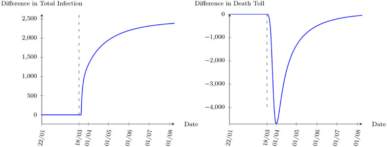
As the collapse of a health care system could lead to a dramatic increase in death rates, it would be of interest to examine how medical capacity affects the results. We experiment it by doubling ω after the calibration periods and find that the results are very similar to the benchmark simulation. As shown in Fig. 11 , although an increase in medical capacity lowers immediate death toll, it also lowers the penalty of being infected. In response, people optimally reduce the time staying at home, leading to an increase in infection cases. This then further increases the demand of medical services. As a result, there are no long run effects as shown in Table 4 .

Fig. 11.

Increasing Medical Capacity Simulation, 22 January to 8 August, 2020.

Table 4.

Summary - medical capacity.

	Peak	End	Infection (End)	Death Toll (End)	NLI
Benchmark	22-Mar-20	29-Aug-22	21,171,782	3,797,870	0.181
doubling ω	22-Mar-20	29-Aug-22	21,174,223	3,797,945	0.181

5.4. Hybrid policy

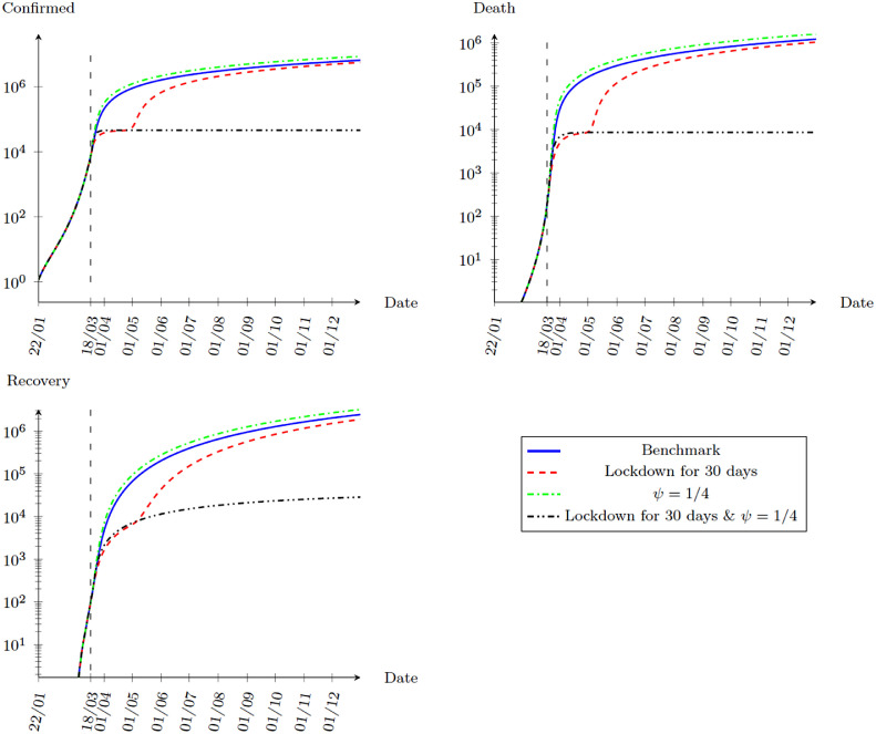
All the simulation results above are showing discouraging results in stopping the epidemic. However, the reason of the failure of lockdown is that lockdown stops the transmission of virus without identifying the infected, but the virus starts to spread again when reopening. Broadening testing identifies those who are infected and lowers the proportion of the infected population in the community. However, as people do not internalize the social costs of spreading the virus, they return to normal life too soon under a lowered infection probability due to broadening testing. Hence, the two policies work together, with broadening testing lowering the risk of infection and lockdown restricting people from returning to normal life too soon. In this part, we experiment again the rapid and target testing with $\psi =1/4$ together with a lockdown of 30 days. Fig. 12 shows the hope to stop the epidemic as lockdown and testing together limit the spread after reopening. The epidemic peaks at 19 March, 2020 when the lockdown starts and end at 18 April, 2020 when the lockdown ends. People return to normal life with NLI equal to 1.

Fig. 12.

Simulation with Lockdown and Broaden Testing, 22 January to 31 December, 2020.

6. Robustness tests

In this section, we perform the robustness tests for the parameters of interests, namely ζ and ν. In our benchmark, we assume $\zeta =0$ and $\nu =0.5$. These two parameters could have important implications on the results. We thus perform a sensitivity analysis for these two parameters. Since ζ and ν are not policy parameters, changing their values would require a re-calibration of the model. In all the results below, we simply re-calibrate the model using the same procedure as that for the benchmark model.

6.1. Temporary immunity

In the benchmark simulation, we assume that $\zeta =0,$ meaning that whoever catch the disease and recovered are granted with immunity forever. However, the lasting of the immunity has important implications on when the epidemic will peak and end.

If recovered individual are susceptible to the virus again in one year on average, ζ is equal to 1/365. As we can see from Table 5 , the possibility of losing immunity significantly worsens the situation. The end of the epidemic prolongs by about 7 months, and both the number of total infection and death toll raise by more than 23%.

Table 5.

Sensitivity results on ζ.

	Peak	End	Infection (End)	Death Toll (End)	NLI (End)
Benchmark	22-Mar-20	29-Aug-22	21,171,782	3,797,870	0.181
$\zeta =1/365$	22-Mar-20	23-Mar-23	26,080,659	4,686,957	0.176

6.2. Relative exposure

In the benchmark, we assume equal exposure probability between outdoor consumption and working away from home with $\nu =0.5$. In this section, we perform two experiments on ν: (1) outdoor consumption leads to more exposure, setting $\nu =1/3,$ and (2) working away from home leads to more exposure, i.e. $\nu =2/3$. From Table 6 , the epidemic worsens if outdoor consumption leads to more exposure, and the situation improves otherwise. The reason is that in the model, working from home is a substitute to commuting to work while there are no close substitutes to outdoor consumption. As a result, if working away from home leads to more exposure ($\nu =2/3$), people will rapidly switch to working from home. However, people are more reluctant to switch away from outdoor consumption even if it has a higher exposure risk ($\nu =1/3$).

Table 6.

Sensitivity results on ν.

	Peak	End	Infection (End)	Death Toll (End)	NLI (End)
Benchmark	22-Mar-20	29-Aug-22	21,171,782	3,797,870	0.181
$\nu =1/3$	23-Mar-20	18-Sep-22	22,905,961	4,112,186	0.168
$\nu =2/3$	22-Mar-20	14-Aug-22	19,733,954	3,538,916	0.259

7. Conclusion

In this paper, we have constructed an extended SIR model with agents optimally choosing outdoor activities. We calibrate the model and match it with the data in the United States. The model predicts the epidemic in the United States very well. The counterfactual experiments suggest that any single policy alone, including lockdown, broadening COVID-19 testing, and expanding medical capacity, is not effective in tackling the epidemic. Lockdown is not as effective as many people believe because people will optimally reduce outdoor activities if the risk of being infected is high. When the economy reopens after the lockdown, the infection risk is low, and people respond by increasing their outdoor activities. This will negate almost all the effects brought by the lockdown if there are still infected individuals in the community. Broadening testing gives incentives for people to return to their normal life as fewer infected individuals are outside hanging around. However, as people do not internalize the social cost of returning to normal life, the situation can get even worse. We also find that increasing medical capacity will only have temporary effects on reducing the death toll. As the cost of infection decreases, more people hang around and infection increases as a result. The most effective policy is a combination of lockdown and broadening testing: Broadening testing lowers the risks of infection, and lockdown further prevent people from returning to normal life too early. Our result shows that a lockdown of 30 days together with a shortening of the duration between being exposed to the virus and being tested positive from an average of nine days to four days can successfully defeat the epidemic. Finally, under the benchmark simulation without any policy intervention, the epidemic peaks on 23 March, 2020 and ends on 19 August, 2022. However, the epidemic will be prolonged by another seven months if recovered people lose their immunity in one year on average.

CRediT authorship contribution statement

Wung Lik Ng: Conceptualization, Methodology, Software, Validation, Formal analysis, Investigation, Data curation, Writing - original draft, Writing - review & editing, Visualization.

References

- Alon T.M., Doepke M., Olmstead-Rumsey J., Tertilt M. 2020. The impact of COVID-19 on gender equality. [Google Scholar]; NBER Working Paper No. w26947
- Alvarez F., Argente D., Lippi F. 2020. A simple planning problem for COVID-19 lockdown. [Google Scholar]; NBER Working Paper No. w26981
- Atkeson A. 2020. What will be the economic impact of COVID-19 in the US? Rough estimates of disease scenarios. [Google Scholar]; NBER Working Paper No.w26867
- Aum S., Lee S., Shin Y. 2020. Inequality of fear and self-quarantine: is there a trade-off between GDP and public health? [Google Scholar]; NBER Working Paper No.w27100
- Berger D., Herkenhoff K., Mongey S. 2020. An SEIR infectious disease model with testing and conditional quarantine. [Google Scholar]; NBER Working Paper No.w26901
- Bethune Z., Korinek A. Covid Economics Vetted and Real-Time Papers. CEPR; 2020. COVID-19 infection externalities: pursuing herd immunity or containment? [Google Scholar]
- Chen N. Epidemiological and clinical characteristics of 99 cases of 2019 novel coronavirus pneumonia in Wuhan, China: a descriptive study. Lancet. 2020;395(10223):507–513. doi: 10.1016/S0140-6736(20)30211-7. [DOI] [PMC free article] [PubMed] [Google Scholar]
- Delaporte I., Pena W. 2020. Working from home under COVID-19: Who is affected? Evidence from latin american and caribbean countries. [Google Scholar]; GLO Discussion Paper No.528
- Dingel J., Neiman B. 2020. How many jobs can be done at home. [DOI] [PMC free article] [PubMed] [Google Scholar]; NBER Working Paper No.w26948
- Eichenbaum M., Rebelo S., Trabandt M. 2020. The macroeconomics of epidemics. [Google Scholar]; NBER Working Paper No.w26882
- Favero, C., 2020. Why is COVID-19 mortality in lombardy so high? Evidence from the simulation of a SEIHCR model.
- Garibaldi P., Moen E., Pissarides C. Covid Economics Vetted and Real-Time Papers. CEPR; 2020. Modelling contacts and transitions in the SIR epidemics model. [Google Scholar]
- Gonzalez-Eiras M., Niepelt D. 2020. On the optimal ‘lockdown’ during an epidemic. [Google Scholar]; CESifo Working Paper No.8240
- Gottlieb C., Grobovsek J., Poschke M. Covid Economics Vetted and Real-Time Papers. CEPR; 2020. Working from home across countries. [Google Scholar]
- Guan W. Clinical characteristics of coronavirus disease 2019 in China. N. Engl. J. Med. 2020;382(18):1708–1720. doi: 10.1056/NEJMoa2002032. [DOI] [PMC free article] [PubMed] [Google Scholar]
- Krueger D., Uhlig H., Xie T. 2020. Macroeconomic dynamics and reallocation in an epidemic. [Google Scholar]; NBER Working Paper No.w27047
- Saltiel F. Covid Economics Vetted and Real-Time Papers. CEPR; 2020. Who can work from home in developing countries? [Google Scholar]
- Toda, A., 2020. Susceptible-infected-recovered (SIR) dynamics of COVID-19 and economic impact. arXiv:2003.11221.
- Wang H. Phase-adjusted estimation of the number of coronavirus disease 2019 cases in Wuhan, China. Cell Discov. 2020;6(1):1–8. doi: 10.1038/s41421-020-0148-0. [DOI] [PMC free article] [PubMed] [Google Scholar]
- Wu Z., McGoogan J. Characteristics of and important lessons from the coronavirus disease 2019 (COVID-19) outbreak in China. JAMA. 2020;323(13):1239–1242. doi: 10.1001/jama.2020.2648. [DOI] [PubMed] [Google Scholar]