Deep Feature Stability Analysis Using CT Images of a Physical Phantom Across Scanner Manufacturers, Cartridges, Pixel Sizes, and Slice Thickness

Abstract

Image acquisition parameters for computed tomography scans such as slice thickness and field of view may vary depending on tumor size and site. Recent studies have shown that some radiomics features were dependent on voxel size (= pixel size × slice thickness), and with proper normalization, this voxel size dependency could be reduced. Deep features from a convolutional neural network (CNN) have shown great promise in characterizing cancers. However, how do these deep features vary with changes in imaging acquisition parameters? To analyze the variability of deep features, a physical radiomics phantom with 10 different material cartridges was scanned on 8 different scanners. We assessed scans from 3 different cartridges (rubber, dense cork, and normal cork). Deep features from the penultimate layer of the CNN before (pre-rectified linear unit) and after (post-rectified linear unit) applying the rectified linear unit activation function were extracted from a pre-trained CNN using transfer learning. We studied both the interscanner and intrascanner dependency of deep features and also the deep features' dependency over the 3 cartridges. We found some deep features were dependent on pixel size and that, with appropriate normalization, this dependency could be reduced. False discovery rate was applied for multiple comparisons, to mitigate potentially optimistic results. We also used stable deep features for prognostic analysis on 1 non–small cell lung cancer data set.

Introduction

In medical research, imaging plays an important role in identifying abnormalities by creating a visual depiction of the internal organs of the human body for clinical analysis. Radiomics (1, 2) refers to the extraction of quantitative features from medical images to discover prognostic or diagnostic disease markers. These features may have the ability to enable building classifiers for effective detection, diagnosis, and therapy outcome prediction of cancer.

Computed tomography (CT) scans are used extensively in cancer diagnosis and treatment. CT scans between patients may have different acquisition and reconstruction parameters. These parameters vary among scanner vendors as well. In addition, every institution follows its own scan protocols; therefore, scans for the same body part may differ among institutions. As a result, a radiomics prediction model generated on one institution's data may not be usable or may not generate acceptable performance with another institution's data. Hence, it is necessary to analyze the stability of features under varying imaging parameters to assess the impact of the latter on the former.

Most reports on the stability and robustness of radiomics features with variation in image acquisition parameters are on patients' CT scans. In a previous study (3), we analyzed the variability and stability of radiomics features across different image acquisition parameters using 8 scanners from 3 different manufacturers. The acquired images had 7 different pixel sizes ranging from 0.39 to 0.98 mm, and the slice thickness varied from 1.25 to 3.75 mm. It was found that some radiomics features were voxel size–dependent, but with a proper normalization approach, this dependency could be reduced or eliminated. Galavis (4) analyzed the variability of texture features under various acquisition and reconstruction parameters using 20 patients with solid tumors. In total, 50 texture features were extracted and further classified into 3 groups based on variation range: small variability features (range ≤ 5%), intermediate variability features (10% ≤ range ≤ 25%), and large variability features (≥30%). Hunter (5) analyzed radiomics features that were stable and informative across different machines using 56 patients with non–small cell lung cancer (NSCLC) from 3 CT scan machines of 2 institutions. The Jaccard index and dice similarity coefficient were used to analyze the stability of radiomics features across multiple machines. He found that redundancy and stability of features depended on the CT image type and CT scanner. Balagurunathan (6) analyzed the stability of features from CT scans of 32 patients with NSCLC. Baseline and follow-up scans of the patients were obtained within a gap of 15 minutes using the same CT scanner and imaging protocol. There were 23 stable features out of a total of 219 features extracted. To show the prognostic potential of these 23 features, another independent NSCLC data set with 59 lung adenocarcinomas was used.

Every scanner has its own set of image acquisition and reconstruction parameters as shown in Table 1. The variability of image acquisition and reconstruction parameters across different machines could be measured to enable adjustments by scanning a given patient multiple times with different sets of imaging parameters for each machine. However, scanning the same patient multiple times is ethically questionable owing to the accumulated ionizing radiation dose. To address this problem, a physical phantom can be used to acquire multiple scans while varying imaging parameters for different machines. Zhao et al. (7) analyzed 22 phantom lesions for exploring slice thickness and reconstruction kernel variation using 14 radiomics features. In total, 3 different slice thicknesses (1.25, 2.5, and 5 mm) and 2 reconstruction kernels were used to obtain the scans. They observed that all features were significantly different when imaged at 1.25-mm versus 5-mm slice thickness and suggested that thinner (1.25 and 2.5 mm) and thicker (5 mm) slice images should not be used concurrently. Mackin et al. (8) investigated the interscanner variability of radiomics features using phantoms by obtaining scans from 17 different scanners. In total, 20 patients with NSCLC were also used to measure the variability of features from tumors. They concluded that the variability of some radiomics features extracted from NSCLC tumors was comparable to the variability of the same radiomics features obtained from CT scans of phantoms across different CT scanners. We also previously studied the variation of feature values across different scanners for several manufacturers (3).

Table 1.

CT Scanners and Scanner Parameters Used in This Study

Scanner	kVp	mAs	ScanType	Pitch	RotationTime(Sec)	ReconstructionKernel	DetectorConfiguration(mm)	SliceThickness(mm)
GE Discovery STE (GE1)a	120	250b	Helical	0.984	1.0	Standard	Det. Coverage = 40	1.25, 2.5, and 3.75
GE LightSpeed 32 pro (GE2)	120	250b	Helical	0.984	1.0	Standard	Det. Coverage = 40	1.25, 2.5, and 3.75
Philips Big Bore (P1)	120	250	Helical	1.024	1.0	Standard (B)	16 × 0.75	1.5, 2, and 3
Philips Brilliance 64 (P2)	120	250	Helical	1.024	1.0	Standard (B)	64 × 0.625	1.5, 2, and 3
Siemens Definition As (S1)	120	250	Helical	1.0	1.0	I31f-2	64 × 0.625	1.5, 2, and 3
Siemens Sensation 64 (S2)	120	250	Helical	1.0	1.0	B31f	64 × 0.625	1.5, 2, and 3
Siemens Sensation 40 (S3)	120	250	Helical	1.0	1.0	B31f	40 × 0.625	1.5, 2, and 3
Siemens Sensation 16 (S4)	120	250	Helical	1.0	1.0	B31f	16 × 0.75	1.5, 2, and 3

^aGE1 (GE Discovery STE) was a PET/CT scanner.

^bFor GE scanners, manual mAs were used; for all other scanners, quality reference mAs were used.

In recent years, with the advancement of neural networks (9, 10), deep features obtained from deep neural networks have been proposed for analyzing cancerous tumors alone or in combination with conventional radiomics features. One of the most crucial traits of deep features to qualify as a potential imaging biomarker is stability across scans. Until now, there was not much work regarding deep features' variability over scanner parameters other than our previous work (11), in which prerectified linear unit (pre-ReLU) features (deep features from the layer before the outputs of a pretrained convolutional neural network [CNN] before applying the ReLU activation function) were used for the analysis of deep feature variability. Our current work is an extension of our previous work on deep feature stability analysis. In this paper, we have made the following contributions using the following CT radiomics phantom images:

1. In total, 8 different scanners from 3 different manufacturers were investigated in our current study.

2. As post-ReLU features have shown better classification performance (12), along with the pre-ReLU features, these were also examined for stability analysis.

3. In our previous work, only the rubber cartridge, which showed textural similarity to NSCLC tumors, was used. The dense cork cartridge also showed textural similarity to NSCLC tumors (13). In this study, we examined dense cork and natural cork cartridges in addition to the rubber cartridge.

4. As the rubber cartridges had Hounsfield unit (HU) values similar to those of NSCLC tumors, the stable deep features for the rubber cartridge were also tested on the 2 other cartridges for classification analysis.

The goal of this study was to analyze the stability of deep features extracted from CT scans (images) from 3 different manufacturers with different image acquisition parameters and to evaluate the stable features' utility in building accurate classifiers.

Materials and Methods

Image Acquisition and Reconstruction

The credence cartridge radiomics (CCR) phantom reported by Mackin (8) was used in image acquisition. In total, 8 different scanners from 3 different manufacturers (GE, Philips, and Siemens) were used to obtain scans using the CCR phantom at the H. Lee. Moffitt Cancer Center and Research Institute, Tampa, FL. Slice thicknesses for the GE scanners were 1.25, 2.5, and 3.75 mm, and those for the Philips and Siemens scanners were 1.5, 2, and 3 mm. The adjacent reconstruction interval or zero interslice gap was used for all CT phantom scans. For every slice thickness, the reconstruction field of view (FOV) varied from 200 to 500 mm (200, 250, 300, 350, 400, 450, and 500 mm) corresponding to pixel sizes ranging from 0.39 to 0.98 mm. The pixel size was calculated as FOV/matrix size, and a matrix size of 512 ×512 was kept constant for all scans. Parameters for each scanner are shown in Table 1. CT (HU) numbers and SDs for different cartridges within the CCR phantom are reported in online supplemental Table 1). The noise power spectrum (NPS) of the rubber cartridge using 5 different scanners was reported in a recent paper (14) for the same pixel sizes and slice thicknesses. The NPS provides the noise texture of an image. Noise texture in a CT image varies with variation of slice thickness, pixel size, and reconstruction kernels. Here, we want to point out that NPS can be used to quantify the noise texture introduced because of different imaging parameters. For example, when the same slice thickness has similar noise texture, it results in similar NPS values. So, noise texture is intrinsically associated with images, while NPS is an analytical tool to quantify that texture. The investigation of the impact of noise on deep features could be significant and thus needs future evaluation. For the same pixel size and slice thickness, CT images might provide the same NPS and thus similar noise texture. However, for different kernels, the NPS, as well as the noise texture, will be different.

Convolutional Neural Networks and Transfer Learning

A CNN (9, 10) is a variant of feedforward neural networks, and it has been used extensively for object recognition and classification. A CNN typically consists of ≥1 convolutional layers along with pooling layers followed by ≥1 fully connected layers, as in a classical multilayer feedforward network. Each neuron has a bias input, accepts some input values on weighted links, executes a dot product, and forwards the output to the next layer. A nonlinear activation function is normally used on the outputs.

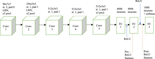
Training a CNN from scratch requires a large amount of data (preferably hundreds of images per class, eg, ImageNet data set). In medical imaging, obtaining a large amount of data (ie, a large number of images) is often difficult. To counter this problem, a transfer learning approach (15, 16) has been used. Using previously learned knowledge to solve a new task is known as transfer learning. In this study, we chose 1 CNN (visual geometry group-slow [VGG-S]) (17) already trained using natural camera images from the ImageNet data set (18). The VGG-S CNN architecture is shown Figure 1. This pretrained CNN has 5 convolution layers followed by 3 fully connected layers. We obtained deep features from the penultimate layer of the CNN before (pre-ReLU) and after (post-ReLU) applying the ReLU activation function. The frequently used ReLU activation function for a CNN is represented by the following equation:

$$f=\text{max}\left(0,x\right)=\left\{\begin{array}{c}x,if{x}_{}\ge 0\\ 0,if{x}_{}<0\end{array}\right.$$

where x is the feature value. Notice that after applying the ReLU activation function, negative feature values are set to 0 and positive feature values remained unchanged.

Figure 1.

Visual geometry group-slow (VGG-S) architecture containing 5 convolution layers, conv 1–conv 5, and 3 fully connected layers. A × K × K means subimages created using a K × K kernel; st. indicates convolution stride; LRN indicates local response normalization; pad indicates padding; pool indicates max pooling; and ReLU indicates rectified linear units.

Contouring and Feature Extraction

The phantom had 10 different cartridges, from which we chose rubber, dense cork, and natural cork cartridges for our experiments. We analyzed the rubber and dense cork cartridges because of the similarity of their HU to NSCLC HU values (13), and natural cork was also investigated owing to some visible textural patterns. Throughout the scanning procedure, a 512 × 512 image size was used. Contouring of regions of interest (ROIs) was done with the help of Mirada software (3) (the central region of each cartridge was captured with a spherical ROI of volume 4.2 cm³.) As this was a 2D approach, for every scan of the phantom using a different pixel size and FOV, 1 slice from each of the 3 cartridges was chosen for analysis.

The input image size for the pretrained network was 224 × 224; so, a subimage of the required size was extracted from the center of the 512 × 512 scanned image. The pretrained CNN was trained using color camera images (24-bit images), whereas the phantom's images were grayscale. Hence, deep features were extracted by feeding phantom images through the red channel only (zeros were sent through green and blue channels). The vector size of the extracted deep features was 4096 (12). After extraction, deep features were normalized between 1 and −1. Figure 2 shows a phantom image slice of a rubber cartridge and 224 × 224 extracted subregions from different cartridges.

Figure 2.

Phantom image slice of the rubber cartridge (A), 224 × 224 extracted region from rubber cartridge (B), 224 × 224 extracted region from dense cork cartridge, and (C) 224 × 224 extracted region from normal cork cartridge (D) .

Feature Normalization

Using 1 cartridge of the phantom at a time (rubber, dense cork, or normal cork) for every scanner, we obtained scans of 3 different slice thicknesses and, for each slice thickness, 7 different pixel sizes. For every cartridge, 21 different scans were generated with the intent to analyze the stability of each deep feature across these scans.

The deep features were normalized by pixel area and voxel size using the following equations (according) to our previous studies (3, 11):

$$f_n=p^2\times f$$ [1]

$$f_{nv}=p^2\times t\times f,$$ [2]

where f_n and f_nv are the normalized feature value by pixel area and voxel size, respectively; p is the pixel size; t is the slice thickness; and f is the original feature value.

For each of the 4096 features, the concordance correlation coefficient (CCC) (19) across the 21 scans was calculated with respect to the pixel size before and after feature normalization. The maximum CCC after feature normalization was around 0.8 for some deep features, whereas those same features had much lower CCC (∼0.3) before feature normalization. As the CCC values could be low even after normalization, improvements in the CCC values after normalization were noted. Each CCC value was converted to a z value (using Fisher transformation equation [3] (20), and the improvement was calculated by equation [4]. After that, the z value was converted to a P-value, and the improvement significance was checked at the 95% significance level, P = .05. If any feature was found to be improved with a P >.05, then that feature was not evaluated further. Equations [3] and [4] are as follows:

$$Z=0.5\times {\text{log}}_e\frac{1+r}{1-r}$$ [3]

$$Z_{diff}=\frac{Z1-Z2}{\sqrt{\frac{1}{n-3}+\frac{1}{m-3}}},$$ [4]

where r is the CCC value; Z is the transformed z value obtained from a CCC; Z1 and Z2 are the transformed z values obtained from the CCC of the original deep feature and the normalized deep feature, respectively; and n and m are the number of data points for every feature (here it is 21 for 7 pixel sizes and 3 slice thicknesses).

After using CCC for further filtering, the SD was also computed for each feature after normalization. Stability was determined using thresholds as follows. A threshold value of 0.25 was chosen for the SD. If a feature value had an SD <0.25, that feature value was considered stable across different pixel sizes. The chosen threshold value encompassed 12.5% of the feature range. The SD threshold will mostly rule out features that have widely disparate values but will vary little, on average. After normalization, a feature will be called stable with respect to a change of pixel size, if it had P-values <.05 and <.25 for its CCC and SD, respectively.

For the stability analysis, 4096 deep features were extracted from the pretrained CNN. This large number has the problem of multiple comparisons potentially showing spurious results. To avoid this, false discovery rate (FDR) (22) was applied to the discovered stable features to adjust their P-value.

Experiments and Results

In Section 3, the results of multiple scans of cartridges are analyzed for deep feature stability. If a feature varies with the change of pixel size or voxel size, then a machine learning model built with deep features extracted using one institution's data may not work on another institution's data. Stable features are needed across different scanner parameters. We called a feature stable if, after normalization, the feature had a similar value within a chosen threshold limit independently of scanner parameters, which meant that the feature was stable across variations of parameters.

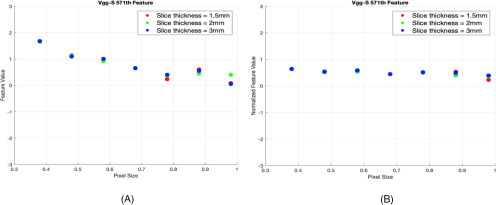
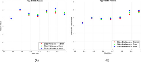
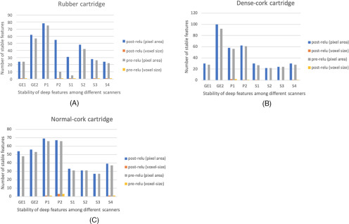
Based on both SD and improvement in CCC, we grouped the deep features into 2 different groups. Group 1 consisted of features whose improvement in CCC resulted in P-value and SD values <.05 and <0.25, respectively. These features showed less variability with the change of pixel sizes and slice thicknesses, and they were considered stable across pixel sizes. Group 2 comprised unstable features that did not become stable after applying normalization (ie, showed variability before and after normalization). We analyzed the stability of deep features for both pre-ReLU and post-ReLU features extracted from 3 different phantom cartridges. Figures 3 and 4 show examples of a feature that improved and of one that did not improve after normalization, respectively. Figure 5A shows stability results of VGG-S pre-ReLU and post-ReLU features obtained from the rubber cartridge. Figure 5B shows the analysis of the dense cork, and Figure 5C describes results from the normal cork.

Figure 3.

Feature improvement by normalization. Before normalization (SD = 0.49) (A) and after normalization using pixel area (SD = 0.1 and false discovery rate [FDR] corrected P = .045) (B) (post-VGG-S features from Philips Brilliance 64 scanner and dense cork cartridge).

Figure 4.

Feature that did not improve by normalization. Before normalization (SD = 0.38) (A) and after normalization using pixel area (SD = 0.48) (B) (pre-VGG-S features from Philips Brilliance 64 scanner and dense cork cartridge) (y-axis represents feature value and x-axis represents pixel size).

Figure 5.

Results from rubber cartridge (A), dense cork (B), and normal cork cartridge (C) (only the number of features that are stable are shown).

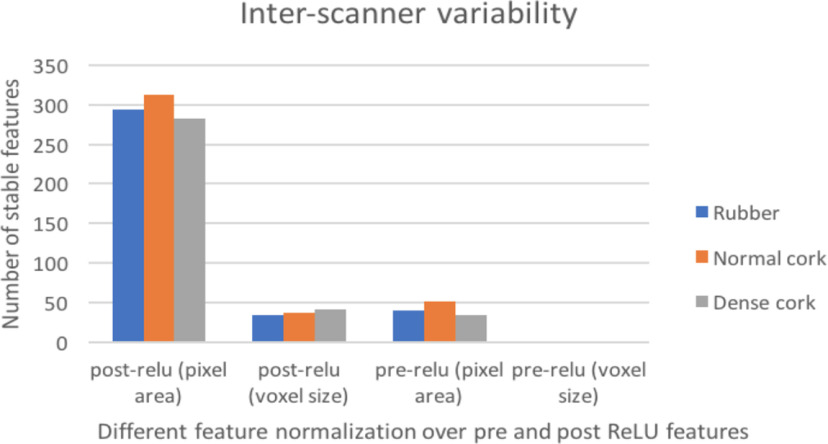
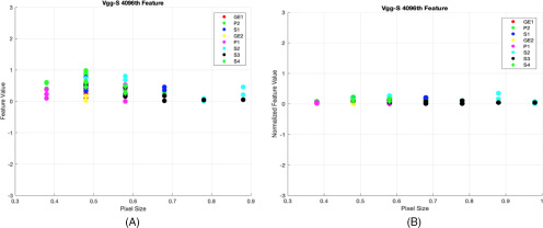
We observed that normalization using the pixel area helped to obtain more stable features (reducing variations and increasing stability across different pixel sizes) better than normalization using voxel size. After analyzing intrascanner dependency (investigating features from every scanner separately), we analyzed features from different scanners jointly (interscanner dependency). Interscanner dependency evaluates the number of stable features by comparing all 4096 features among all scanners. Different cartridges (rubber, dense cork, and normal cork), normalization approaches, and deep features (post-ReLU and pre-ReLU) were also compared. Figure 6 shows the results obtained from the interscanner dependency analysis. Only 1 pre-ReLU feature obtained from different scanners was found to be stable across 3 cartridges. Whereas for post-ReLU features, 19 features were found to be stable across 3 cartridges. Figure 7 shows a feature found to be stable after normalization (interscanner dependency).

Figure 6.

Results from interscanner stability (only the number features that are stable are shown in the figure).

Figure 7.

Inter-scanner dependency (post-ReLU 4096th feature using rubber cartridge): feature improvement after normalization, before normalization (SD = 0.28) (A), after normalization using pixel area (SD = 0.1 and FDR corrected P-value = .0024) (B). [Note: In figure, GE1 = GE Discovery STE, GE2 = GE LightSpeed 32 pro, P1 = Philips Big Bore, P2 = Philips Brilliance 64, S1 = Siemens Definition As, S2 = Siemens Sensation 64, S4 = Siemens Sensation 40, and S4 = Siemens Sensation 16].

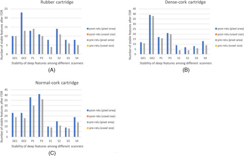
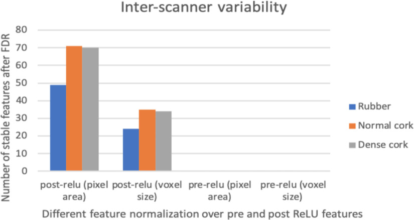
FDR was applied on the discovered stable features to adjust their P-value. Now the features with adjusted P-value were compared against those with P-value of .05. After the FDR correction, the number of stable features was reduced (49, 71, and 70 deep features were stable on rubber, dense cork, and normal cork cartridges, respectively). Interscanner dependency (analysis of features obtained from different scanners) was also explored. Each of these 3 cartridges had different HU values and textures. Only 1 post-ReLU feature (feature column 299) from CNN was found to be stable across different scanners for all 3 cartridges after P-values were corrected using FDR. The stability of features changed significantly with the change of cartridges. Hence, the question of stability on a cartridge was examined. The results obtained after applying FDR are shown in Figures 8 and 9.

Figure 8.

Results after using FDR: rubber cartridge (A), dense cork (B), and normal cork cartridge (C) (only the number of features that are stable are shown).

Figure 9.

Results from interscanner stability after FDR (only the number features that are stable are shown in the figure).

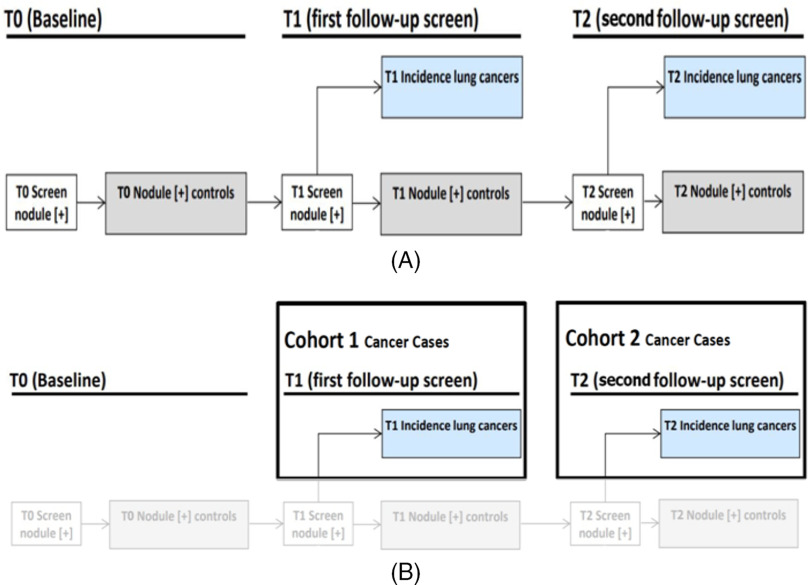
One data set was chosen to analyze the relevant utility of the stable deep features for prognostic analysis. Deidentified data from the National Lung Screening Trial (NLST) was obtained via the data access system of the National Cancer Institute under an IRB-approved process. Figure 10 describes the NLST study timeline as well as the criteria for dividing the SDLCs and NPCs into Cohort1 and Cohort2. It should be noted that the scans performed on the physical phantom (120 kVp, 250 mAs) were not equivalent to the low-dose scans used on the NLST data set (120–140 kVp, 40–80 mAs). Nevertheless, we have shown that stable deep features identified using phantom images can be used to enhance malignancy classification in humans during low-dose CT screening, which uses a higher mAs value. A detailed description of the data set is in the online supplemental Appendix (23, 24) which includes Figure 10 describing the data. Deep features from the CNN were extracted using the red-color channel. In our previous study (21), we experimented with the original deep features (without choosing any stable features) and the top 5 / 10/15 / 20 deep features were selected using the symmetric uncertainty (25) feature selector. In Paul et al.'s study (21), using VGG-S deep features from the red-color channel gave the best classification accuracy of 65.4% with 0.66 area under the curve (AUC) using 15 features.

Figure 10.

National Lung Screening Trial (NLST) study and (A) flowchart of selection of cohort 1 and cohort 2 from the NLST study (B).

The deep features (49) that were found to be stable on rubber cartridges over different scanners and parameters were evaluated further to determine whether the use of stable features could lead to improved classification performance. The classification performance was evaluated with respect to accuracy and area under the receiver operating characteristic curve (26). We also choose the top 5 / 10/15 / 20 deep features from our stable features using the symmetric uncertainty feature selector and using all 49 features to classify using random forests classifier (27). We found that using pixel area normalized deep features enabled 67.08% accuracy with 0.67 AUC, which was an improvement over our previous analysis using all 4096 features. The classification performance was further enhanced to 68.77% (0.68 AUC) by using all 49 stable features, a 2% accuracy increase over using unnormalized features. Detailed results are shown in Table 2. Online supplemental Appendix Table 2) compares the performance of different classifiers [decision tree (28), naïve Bayes (29), and nearest neighbors (30)] with unmodified deep features and normalized stable deep features. From this study, we observed the importance of deep feature stability assessment before prognostic evaluation. By choosing the stable features, we may avoid using unreliable and irrelevant features.

Table 2.

Malignancy Prediction Results Using NLST Data set

# of Features	Original Deep Features(All 4096 Features)a	Stable DeepFeatures Onlyb	Stable Deep Features – Normalizedby Pixel Areab
Top 5	62.02 (0.643)	64.135 (0.62)	62.02 (0.6)
Top 10	63.71 (0.66)	63.71 (0.66)	65.4 (0.64)
Top 15	65.4 (0.66)	65.82 (0.66)	65.4 (0.66)
Top 20	64.97 (0.66)	66.24 (0.66)	67.08 (0.67)
Top 49 or All 49	66.24 (0.68)	67.08 (0.68)	(0.68)

^aTop 49 features were chosen here using feature selector.

^bAll 49 features were stable deep features obtained from rubber cartridge.

Discussion

CT imaging plays a critical role in current NSCLC treatment and research. The FOV can vary from scan to scan depending on the size, location, and NSCLC tumor stage and patient size. Slice thickness is another important parameter selected for obtaining a scan. How these image acquisition parameters affect features extracted from a CNN remains unexplored. Hence, the main focus of this study was to evaluate how deep features behave with variation in image acquisition parameters. There has been recent work (31) on finding semantic meaning for deep features, suggesting that meaning may be ascertained for stable deep features. To the best of our knowledge, this is the first work analyzing the stability of deep features with varying slice thickness and FOV. In this paper, only pixel size and slice thickness dependency and variability were chosen for analysis. The goal was to gain a better understanding of the variability and allow focus on ways to remove or reduce variability.

In our previous study (21), deep features extracted from different color channels of a pretrained CNN were analyzed and variations in classification accuracies were also obtained. Deep features were extracted from the red channel of the pretrained CNN (VGG-S) for our current study. VGG-S was chosen for our study because deep features from VGG-S showed good classification for NSCLC nodules (21).

From this study, we observed that some deep features were stable as shown in Figure 4 (small variability with the variation of pixel size) within a chosen threshold. These stable features did not appreciably change with the change of pixel sizes. Some of the deep features were pixel size–dependent. These features showed variation with changes in pixel size. Robust and stable features across different reconstruction kernels and image acquisition parameters are desirable in radiomics. In an attempt to stabilize these features across the variability of pixel sizes, we proposed 2 normalization procedures using pixel area and voxel size (11, 14). In some cases, features stabilized after being normalized by pixel area or voxel size. However, some of these pixel size–dependent features showed variability even after normalization. They were not stable with pixel size. Hence, we found that some deep features also had pixel size dependencies such as the conventional radiomics features, and a similar correction approach could be used to reduce the dependency.

Normalization using pixel area generated a greater number of stable features (less variability across pixel size changes) than using voxel size. In fact, voxel size normalization by itself was of minimal help, perhaps because we are dealing with planar images (2D), 1 slice per scan. It added only a couple more stable features, in some cases, to the set found with pixel area normalization. Voxel size is a volume that may explain the lack of improvement when normalizing by it. Interscanner dependency (analysis of features obtained from different scanners) was also explored. Each of these 3 cartridges (rubber, dense cork, and natural cork) had different HUs and textures, yet 1 pre-ReLU and 19 post-ReLU features from a VGG-S pretrained CNN were found to be stable across different scanners for all 3 cartridges.

Previously (12, 21) we found that using post-ReLU features provided better classification performance than using pre-ReLU features for lung nodules. Post-ReLU features lack negative values (all the negative values were made 0) owing to the ReLU activation function. Pre-ReLU features had negative feature values. Both sets of features (pre- and post-ReLU) were investigated to gain our understanding of feature stability. From our current study, we found more post-ReLU deep features could be stabilized than pre-ReLU features.

We found that the features also changed significantly when using different scanners with different protocols. Our analysis also showed that more deep features from the dense cork cartridges were stable than features from the rubber and normal cork cartridges. This happened because the texture of dense cork cartridge is more uniform than that of the rubber and normal cork cartridges.

Finally, in this study, pre- and post-ReLU features were obtained from a transfer learning approach, which was a limitation of the study because the VGG-S CNN was not trained on any type of medical images or any medical imaging modality. We used transfer learning because we do not yet have the large number of medical images needed to train a complex CNN and to explore the utility of transfer learning. Given our present results, deep features from a CNN trained on CT images will be investigated in the future. Even though phantoms were made of different materials with different texture, an analysis using real human CT scans would be useful. No scans from human subjects were used for stability analysis, which was a limitation of this study. In future work, more analysis using patient data will be analyzed for prognostic evaluation after using the proposed pixel size-based normalization. Deep features from only the red channel of the VGG-S network were used for this study, which was another limitation. In the future, feature normalization will be analyzed during CNN training to determine if it is possible to identify characteristics of features that would benefit from normalization. The deep features will be analyzed further using different scanner parameters and various reconstruction kernels.

Conclusions

The goal of this study was to analyze whether deep features were stable across different scanner parameters and manufacturers. Stability is one of the essential characteristics of deep features to qualify as a potential imaging biomarker. From this study, we found that many deep features were dependent on pixel size, as are many conventional radiomics features. It was found that this dependency could be reduced, for some, by normalizing the deep features using pixel area and voxel size. We found that the stability of deep features changed significantly when using different phantom cartridges (49, 71, and 70 deep features were stable on rubber, dense cork, and normal cork cartridges, respectively). We also looked for deep features that were stable across 3 physical phantom cartridges for post-ReLU, and found 1 feature. The 3 cartridges were made of different components and had differences in texture uniformity and HU values. It is therefore advisable to analyze the stability of deep features among different cartridges independently. The stable and normalized deep features achieved improved classification performance compared with the original deep features chosen by the symmetric uncertainty feature selector, which shows the usefulness of stable features for prognosis analysis. Based on this study, some deep features may be candidates for future imaging biomarkers, but researchers must be cautious because most deep features show dependence on image acquisition parameter variations.

References

- 1. Lambin P, Rios-Velazquez E, Leijenaar R, Carvalho S, Van Stiphout RG, Granton P, Zegers CM, Gillies R, Boellard R, Dekker A, Aerts HJ. Radiomics: extracting more information from medical images using advanced feature analysis. Eur J Cancer. 2012;48:441–446. [DOI] [PMC free article] [PubMed] [Google Scholar]
- 2. Kumar V, Gu Y, Basu S, Berglund A, Eschrich SA, Schabath MB, Forster K, Aerts HJWL, Dekker A, Fenstermacher D, Goldgof DB, Hall LO, Lambin P, Balagurunathan Y, Gatenby RA, Gillies RJ. Radiomics: the process and the challenges. Magn Reson Imaging. 2012;30:1234–1248. [DOI] [PMC free article] [PubMed] [Google Scholar]
- 3. Shafiq-Ul-Hassan M, Zhang GG, Latifi K, Ullah G, Hunt DC, Balagurunathan Y, Abdalah MA, Schabath MB, Goldgof DG, Mackin D, Court LE, Gillies RJ, Moros EG. Intrinsic dependencies of CT radiomic features on voxel size and number of gray levels. Med Phys. 2017;44:1050–1062. [DOI] [PMC free article] [PubMed] [Google Scholar]
- 4. Galavis PE, Hollensen C, Jallow N, Paliwal B, Jeraj R. Variability of textural features in FDG PET images due to different acquisition modes and reconstruction parameters. Acta Oncol. 2010;49:1012–1016. [DOI] [PMC free article] [PubMed] [Google Scholar]
- 5. Hunter LA, Krafft S, Stingo F, Choi H, Martel MK, Kry SF, Court LE. High quality machine‐robust image features: identification in nonsmall cell lung cancer computed tomography images. Med Phys. 2013;40:121916. [DOI] [PMC free article] [PubMed] [Google Scholar]
- 6. Balagurunathan Y, Gu Y, Wang H, Kumar V, Grove O, Hawkins S, Kim J, Goldgof DB, Hall LO, Gatenby RA, Gillies RJ. Reproducibility and prognosis of quantitative features extracted from CT images. Transl Oncol. 2014;7:72–87. [DOI] [PMC free article] [PubMed] [Google Scholar]
- 7. Zhao B, Tan Y, Tsai WY, Schwartz LH, Lu L. Exploring variability in CT characterization of tumors: a preliminary phantom study. Transl Oncol. 2014;7:88–93. [DOI] [PMC free article] [PubMed] [Google Scholar]
- 8. Mackin D, Fave X, Zhang L, Fried D, Yang J, Taylor B, Rodriguez-Rivera E, Dodge C, Jones AK, Court L. Measuring CT scanner variability of radiomics features. Invest Radiol. 2015;50:757–765. [DOI] [PMC free article] [PubMed] [Google Scholar]
- 9. LeCun Y, Boser B, Denker JS, Henderson D, Howard RE, Hubbard W, Jackel LD. Backpropagation applied to handwritten zip code recognition. Neural Computation. 1989;1:541–551. [Google Scholar]
- 10. Zeiler MD, Fergus R. Visualizing and understanding convolutional networks. In: European Conference on Computer Vision. 2014. (pp. 818–833). Springer, Cham. [Google Scholar]
- 11. Paul R, Shafiq-Ul-Hassan M, Moros EG, Gillies RJ, Hall LO, Goldgof DB. Stability of deep features across CT scanners and field of view using a physical phantom. In: Proceedings SPIE, Medical Imaging 2018: Computer-Aided Diagnosis, 105753; February 27, 2018. [Google Scholar]
- 12. Paul R, Hawkins SH, Balagurunathan Y, Schabath MB, Gillies RJ, Hall LO, Goldgof DB. Deep feature transfer learning in combination with traditional features predicts survival among patients with lung adenocarcinoma. Tomography. 2016;2:388–395. [DOI] [PMC free article] [PubMed] [Google Scholar]
- 13. Fave X, Mackin D, Yang J, Zhang J, Fried D, Balter P, Followill D, Gomez D, Kyle Jones A, Stingo F, Fontenot J, Court L. Can radiomics features be reproducibly measured from CBCT images for patients with non‐small cell lung cancer? Med Phys. 2015;42:6784–6797. [DOI] [PMC free article] [PubMed] [Google Scholar]
- 14. Shafiq-Ul-Hassan M, Zhang GG, Hunt DC, Latifi K, Ullah G, Gillies RJ, Moros EG. Accounting for reconstruction kernel-induced variability in CT radiomic features using noise power spectra. J Med Imag. 2017;5:011013. [DOI] [PMC free article] [PubMed] [Google Scholar]
- 15. Oquab M, Bottou L, Laptev I, Sivic J. Learning and transferring mid-level image representations using convolutional neural networks. In: Proceedings of the IEEE Conference on Computer Vision and Pattern Recognition 2014. (pp. 1717–1724). [Google Scholar]
- 16. Thrun S. Is learning the n-th thing any easier than learning the first? Adv Neural Inf Process Syst. 1996:640–646. [Google Scholar]
- 17. Chatfield K, Simonyan K, Vedaldi A, Zisserman A. Return of the devil in the details: delving deep into convolutional nets. In: Proceedings of BMVC 2014; arXiv preprint arXiv:1405.3531 2014. [Google Scholar]
- 18. Deng J, Dong W, Socher R, Li LJ, Li K, Fei-Fei L. Imagenet: a large-scale hierarchical image database. In: 2009 IEEE Conference on Computer Vision and Pattern Recognition 2009. (pp. 248–255). [Google Scholar]
- 19. Lawrence I, Lin K. A concordance correlation coefficient to evaluate reproducibility. Biometrics. 1989;45:255–268. [PubMed] [Google Scholar]
- 20. Dhanoa MS, Lister SJ, France J, Barnes RJ. Use of mean square prediction error analysis and reproducibility measures to study near infrared calibration equation performance. J Near Infrared Spectrosc. 1999;7:133–143. [Google Scholar]
- 21. Paul R, Hawkins S, Schabath MB, Gillies RJ, Hall LO, Goldgof DB. Predicting malignant nodules by fusing deep features with classical radiomics features. J Med Imag. 2018;5:011021. [DOI] [PMC free article] [PubMed] [Google Scholar]
- 22. Benjamini Y, Hochberg Y. Controlling the false discovery rate: a practical and powerful approach to multiple testing. J R Stat Soc Series B Stat Methodol. 1995;57:289–300. [Google Scholar]
- 23. Schabath MB, Massion PP, Thompson ZJ, Eschrich SA, Balagurunathan Y, Goldof D, Aberle DR, Gillies RJ. Differences in patient outcomes of prevalence, interval, and screen-detected lung cancers in the CT arm of the national lung screening trial. PLoS One. 2016;11:e0159880. [DOI] [PMC free article] [PubMed] [Google Scholar]
- 24. Hawkins S, Wang H, Liu Y, Garcia A, Stringfield O, Krewer H, Li Q, Cherezov D, Gatenby RA, Balagurunathan Y, Goldgof D, Schabath MB, Hall L, Gillies RJ. Predicting malignant nodules from screening CT scans. J Thorac Oncol. 2016;11:2120–2128. [DOI] [PMC free article] [PubMed] [Google Scholar]
- 25. Yu L, Liu H. Feature selection for high-dimensional data: a fast correlation-based filter solution. In: Proceedings of the 20th International Conference on Machine Learning (ICML-03) 2003. (pp. 856–863). [Google Scholar]
- 26. Hajian-Tilaki K. Receiver operating characteristic (ROC) curve analysis for medical diagnostic test evaluation. Caspian J Intern Med. 2013;4:627–635. [PMC free article] [PubMed] [Google Scholar]
- 27. Ho TK. Random decision forests. In: Proceedings of 3rd International Conference on Document Analysis and Recognition 1995. (1; pp. 278–282). [Google Scholar]
- 28. Quinlan JR. Decision trees and decision-making. IEEE Trans Syst Man Cybern Syst. 1990;20:339–346. [Google Scholar]
- 29. Lewis DD. Naive (Bayes) at forty: the independence assumption in information retrieval. ECML. 1998. (pp. 4–15). Springer, Berlin, Heidelberg. [Google Scholar]
- 30. Cover T, Hart P. Nearest neighbor pattern classification. IEEE Trans Inform Theory. 1967;13:21–27. [Google Scholar]
- 31. Paul R, Schabath M, Balagurunathan Y, Liu Y, Li Q, Gillies R, Hall LO, Goldgof DB. Explaining Deep Features Using Radiologist-Defined Semantic Features and Traditional Quantitative Features. Tomography. 2019;5:192–200. [DOI] [PMC free article] [PubMed] [Google Scholar]
Associated Data
This section collects any data citations, data availability statements, or supplementary materials included in this article.