Learning to detect anatomical landmarks of the pelvis in X-rays from arbitrary views

Abstract

Purpose

Minimally invasive alternatives are now available for many complex surgeries. These approaches are enabled by the increasing availability of intra-operative image guidance. Yet, fluoroscopic X-rays suffer from projective transformation and thus cannot provide direct views onto anatomy. Surgeons could highly benefit from additional information, such as the anatomical landmark locations in the projections, to support intra-operative decision making. However, detecting landmarks is challenging since the viewing direction changes substantially between views leading to varying appearance of the same landmark. Therefore, and to the best of our knowledge, view-independent anatomical landmark detection has not been investigated yet.

Methods

In this work, we propose a novel approach to detect multiple anatomical landmarks in X-ray images from arbitrary viewing directions. To this end, a sequential prediction framework based on convolutional neural networks is employed to simultaneously regress all landmark locations. For training, synthetic X-rays are generated with a physically accurate forward model that allows direct application of the trained model to real X-ray images of the pelvis. View invariance is achieved via data augmentation by sampling viewing angles on a spherical segment of 120° × 90°.

Results

On synthetic data, a mean prediction error of 5.6 ± 4.5mm is achieved. Further, we demonstrate that the trained model can be directly applied to real X-rays and show that these detections define correspondences to a respective CT volume, which allows for analytic estimation of the 11 degree of freedom projective mapping.

Conclusion

We present the first tool to detect anatomical landmarks in X-ray images independent of their viewing direction. Access to this information during surgery may benefit decision making and constitutes a first step toward global initialization of 2D/3D registration without the need of calibration. As such, the proposed concept has a strong prospect to facilitate and enhance applications and methods in the realm of image-guided surgery.

Introduction

In recent years, the increasing availability of intra-operative image guidance has enabled percutaneous alternatives to complex procedures. This is beneficial for the patient since minimally invasive surgeries are associated with a reduced risk of infection, less blood loss, and an overall decrease in discomfort. However, this comes at the cost of increased task load for the surgeon, who has no direct view onto the patient’s anatomy but has to rely on indirect feedback through X-ray images. These suffer from projective transformation, particularly the absence of depth cues and, depending on the viewing direction, vanishing anatomical landmarks. One of these procedures is percutaneous pelvis fracture fixation. Pelvis fractures may be complex with a variety of fracture patterns. In order to fixate pelvic fractures internally, K-wires must be guided through narrow bone corridors. Numerous X-ray images from different views may be required to ensure a correct tool trajectory [2,24]. One possibility to support the surgeon during these procedures is to supply additional contextual information extracted from the image. Providing additional, “implicit 3D” information during these interventions can drastically ease the mental mapping, where the surgeon has to register the tool in his hand to the 3D patient anatomy using 2D X-ray images only [8,22]. In this case, implicit 3D information refers to data that are not 3D as such, but provides meaningful contextual information related to prior knowledge of the surgeon.

A promising candidate for implicit 3D information is the positions of anatomical landmarks in the X-ray images. Anatomical landmarks are biologically meaningful locations in anatomy that can be readily detected and enable correspondence between specimens and across domains. Inherently, the knowledge of landmark locations exhibits helpful properties: (1) Context is provided, which supports intra-operative decision making, (2) they supply semantic information, which defines correspondences across multiple images, and (3) they might foster machine understanding. For these reasons, anatomical landmarks are widely used in medicine and medical imaging, where they serve as orientation in diagnostic and interventional radiology [7]. They deliver a better interpretation of the patients’ anatomy [28] and are also of interest for image processing tasks as prerequisite to initialize or constrain mathematical models [27]. A non-exhaustive review reveals that anatomical landmarks have been used to guide and model segmentation tasks [10,31], to perform image registration [12], to extract relevant clinical quantitative measurements [19], to plan therapies [14], or to initialize further image processing [16].

Often, knowing the exact location of landmarks is mandatory for the desired application suggesting that landmarks must be labeled manually [28]. Manual labeling is time-consuming, interrupts the clinical workflow, and is subjective, which yields rater dependent results. Although important, anatomical landmark detection is a challenging task due to patient specific variations and ambiguous anatomical structures. At the same time, automatic algorithms should be fast, robust, reliable, and accurate.

Landmark detection methods have been developed for various imaging modalities and for 2D or 3D image data [6,7]. In the following overview, we focus on 2D X-ray images. Landmark or key point detection is well understood in computer vision, where robust feature descriptors disambiguate correspondences between multiple 2D images, finally enabling purely image-based pose retrieval. Unfortunately, the above concept defined for reflection imaging does not translate directly to transmission imaging. For the latter, image and landmark appearance can change fundamentally depending on the viewing direction since the whole 3D object contributes to the resulting detector measurement.

Most of the current landmark detection approaches either predict the landmark positions on the input image directly, or combine these initial estimates subsequently with a parametric or graphical model fitting step [27]. Constraining detection results by models that encode prior knowledge can disambiguate false positive responses. Alternatively, priors can be incorporated implicitly, if multiple landmarks are detected simultaneously by reducing the search space to possible configurations [15]. Wang et al. [28] summarized several landmark detection methods competing in a Grand Challenge, where 19 landmarks have to be detected in 2D cephalometric X-ray images of the craniofacial area, a task necessary for modern orthodontics. Mader et al. [16] used a U-net to localize ribs in chest radiographs. They solved the problem of ambiguities in the local image information (false responses) using a conditional random field. This second step assesses spatial information between the landmarks and also refines the hypotheses generated by the U-net. Sa et al. [21] detected intervertebral discs in X-ray images of the spine to predict a bounding box of the respective vertebrae, by using a pre-trained Faster-RNN and refining its weights. Payer et al. [18] evaluated different CNN architectures to detect multiple landmark locations in X-ray images of hand X-rays by regressing a single heat map for each landmark. In a similar task, another approach used random forests to detect 37 anatomical landmark in hand radiographs. The initial estimates were subsequently combined with prior knowledge given by possible landmark configurations. [23]. For each landmark, a unique random regression forest is trained. In Xie et al., anatomical landmarks were a prerequisite for the segmentation of the pelvis in anterior–posterior radiographs in order to create a 3D patient specific pelvis model for surgical planning. The shape model utilized for this purpose is based on anatomical landmarks [30].

All the presented approaches above assume a single, predefined view onto the anatomy. This assumption is valid for certain applications, where radiographic images in a diagnostic setup are often acquired in standardized views, but is strongly violated when view changes continuously, e.g., in interventional applications or for projection data acquired on trajectories, scenarios in which the view changes continuously. To the best of our knowledge, there exists no approach that is able to detect anatomical landmarks in X-ray images independent of the viewing direction. The view independence substantially complicates the landmark detection problem in X-ray images since object edges vanish and anatomical structures overlap due to the effect of transmission imaging. X-ray transform invariant landmark detection, therefore, bears great potential to aid fluoroscopic guidance.

In contrast to the landmark detection approaches that deliver implicit 3D information, several approaches exist that introduce explicit 3D information. These solutions rely on external markers to track the tools or the patient in 3D [17], consistency conditions to estimate relative pose between X-ray images [1], or 2D/3D registration of pre-operative CT to intra-operative X-ray to render multiple views simultaneously [17,25]. While these approaches have proven helpful, they are not widely accepted in clinical practice. The primary reasons are disruptions to the surgical workflow [8], as well as susceptibility to both truncation and initialization due to the low capture range of the optimization target [11].

In this work, we propose an automatic, purely image-based method to detect multiple anatomical landmarks in X-ray images independent of the viewing direction. Landmarks are detected using a sequential prediction framework [29] trained on synthetically generated images. Based on landmark knowledge, we can (a) identify corresponding landmarks between arbitrary views of the same anatomy and (b) estimate pose relative to a pre-procedurally acquired volume without the need for any calibration. We evaluate our approach on synthetic data and demonstrate that it generalizes to unseen clinical X-rays of the pelvis without the need for re-training. Further, we argue that the accuracy of our detections in clinical X-rays may benefit the initialization of 2D/3D registration. This paper is an extended version of the work presented at the MICCAI 2018 conference [4] and provides a broader background on existing landmark detection research, a comprehensive quantitative analysis of the view invariance on synthetic data and a quantitative evaluation on real X-ray images of cadaveric specimens.

Materials and methods

Network architecture

The sequential prediction framework used in this work has been initially developed for human pose estimation [29]. In the original application, the machine learning task is to detect multiple human joint positions in RGB images. The architecture is abstractly depicted in Fig. 1. Given a single RGB input image, the network predicts multiple belief maps $b_t^p$ for each joint position p ∈ [1, …, P] at the end of every stage t ∈ [1, …, T] of the network. In the first stage, initial belief maps $b_1^p$ are predicted based only on local image information. Image features are extracted using a stack of convolutional and pooling layers with Rectified Linear Units (ReLUs) as activation functions, described by weights w₁. In following stages t ≥ 2, the predicted belief maps $b_t^p$ are obtained by combining local image information extracted by the layers with weights w_p and the prediction results of the preceding stage. Note that this combination is implemented using a concatenation operation. The weights w_p are shared for all stages t ≥ 2. The cost function C is the sum of the L2-losses between the predicted belief maps $b_t^p$ and the ground truth belief maps $b_t^{*}$:

$$C=\sum _{t=1}^T\sum _{p=1}^P{\Vert b_t^p-b_t^{*}\Vert }_2^2$$ (1)

The ground truth belief maps $b_t^{*}$ contain a normal distribution, centered at the ground truth joint position. By design, the network imposes several properties: The key element of the architecture is that the belief maps are predicted based on local image information as well as the results of the preceding stage. This enables the model to learn long-range contextual dependencies of landmark configurations. The belief maps of the first stage $b_1^p$ are predicted only on local image information, which leads to false positive responses due to ambiguities in the local image appearance. The stage-wise application resolves these by implicitly incorporating the characteristic configuration of the landmark positions. Furthermore, the network has a very large receptive field that also increases over stages, which enables the learning of spatial dependencies over long distances. Lastly, the loss over all intermediate predictions $b_t^p$ is computed, which counteracts the vanishing gradient effect and simultaneously guides the network to focus early on the detection task. A drawback of this architecture is the small size of the output belief maps that are downsampled by a factor of around eight compared to the input size.

Fig. 1.

Schematic representation of the convolutional neural network used in this work. A single input image is processed by multiple stages of convolutional and pooling layers, resulting in a stack of belief maps, where each map corresponds to a landmark location. During the stage-wise application, these belief maps are refined

Landmark detection

We exploit the aforementioned advantages of sequential prediction frameworks for the detection of anatomical landmarks in X-ray images independent of their viewing direction. Our assumption is that anatomical landmarks exhibit strong constraints and thus characteristic patterns even in the presence of arbitrary viewing angles. In fact, this assumption may be even stronger compared to human pose estimation if limited anatomy, such as the pelvis, is considered due to rigidity. Within this paper and as a first proof-of-concept, we study anatomical landmarks on the pelvis. We devise a network adapted from [29] with six stages to simultaneously predict 23 belief maps per X-ray image that are used for landmark location extraction, as shown in Fig. 1.

In order to obtain the predicted landmark positions, all predicted belief maps $b_t^p$ are averaged over all stages prior to estimating the position of the landmarks yielding the averaged belief map b^p. We then define the landmark position lp as the position with the highest response in b^p. Since the belief maps are downsampled, the maximum location is computed in a sub pixel accuracy by a maximum likelihood estimation of the Gaussian estimate. If the maximum response in a belief map is below 0.4, the landmarks are discarded since they may be outside the field of view or are not reliably recognized. The implementation was done in Python and TensorFlow. The hyperparameters for the network training are set to 10⁻⁶ for the learning rate and a batch size of one. Optimization was performed using Adam over 30 epochs until convergence in the validation set had been reached.

Data generation

The network training requires a data set of X-ray images with corresponding landmark positions. Manual labeling is infeasible for various reasons: First of all, the labeling process to obtain the required amount of training data is time costly. However, and more importantly, an accurate and consistent labeling cannot be guaranteed in the 2D projection images due to the discussed properties of transmission imaging (vanishing edges, superimposed anatomy). Therefore, we synthetically generated the training data from full body CTs of the NIH Cancer Imaging Archive [20]. In total, 23 landmark positions were manually labeled in 20 CTs of male and female patients using 3D volume renderings in 3D Slicer [5]. The landmark positions have been selected to be clinically meaningful, to have a good visibility in the projection images and to be consistently identifiable on the anatomy. The selected landmarks are depicted in Fig. 2.

Fig. 2.

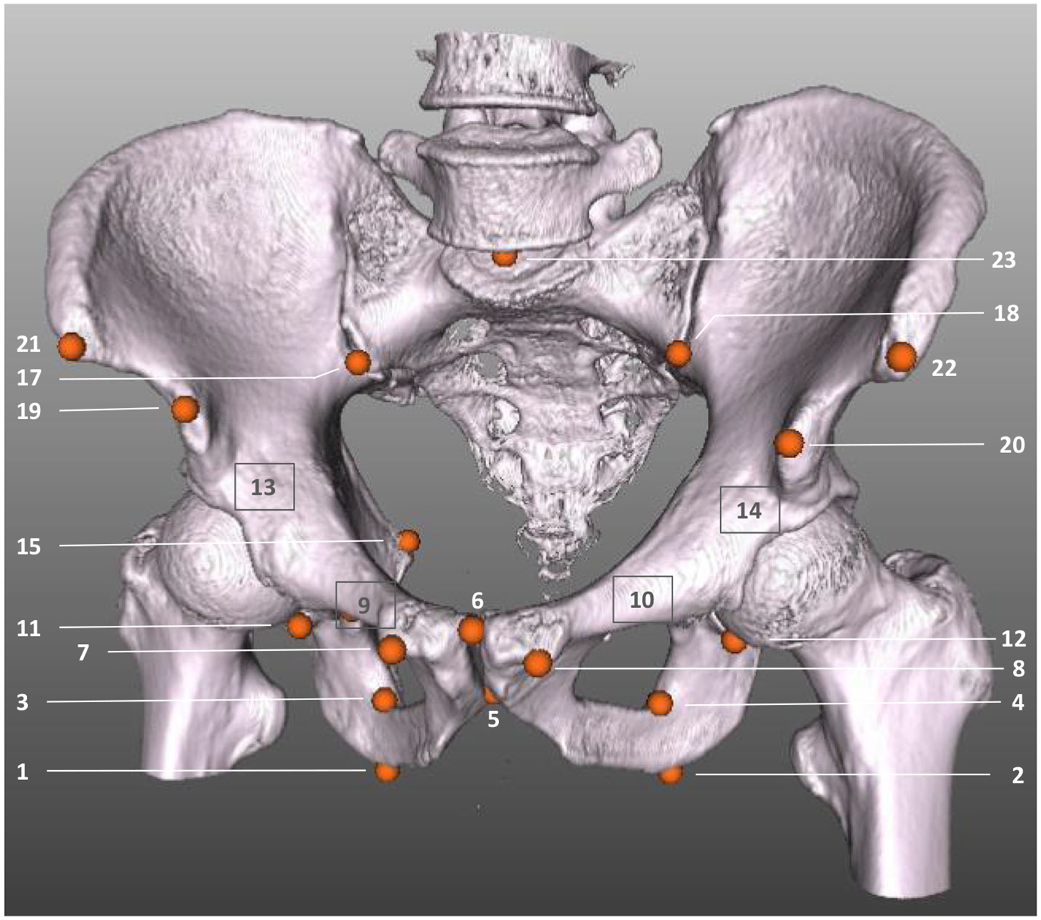
The pelvis bone of a CT of the used data set is rendered with the corresponding 3D landmark labels that have been labeled manually. Orange dots with numbers indicate visible landmarks. Landmarks hidden due to the rendering are marked with a gray box and number (e.g., the tip of the right femoral head, landmark #13)

Subsequently, data were obtained by forward projection of the volume and the respective 3D labels with the same X-ray imaging geometry, resulting in a set of X-ray images with corresponding landmark positions. The synthetic X-ray images had a size of 615 × 479 pixels with an isotropic pixel spacing of 0.616mm. The corresponding ground truth belief maps were downsampled by a factor of about eight and had a size of 76 × 59. For data generation, two factors are important to emphasize: (1) the augmentation of training data in order to obtain view invariance is crucial. To this end, we applied random translation to the CT volume, varied the source-to-isocenter distance, applied flipping on the detector, and most importantly, varied the angular range of the X-ray source position on a spherical segment of 120° in LAO/RAO and in 90° in CRAN/CAUD, centered around an AP view of the pelvis. This range approximates the range of variation in X-ray images during surgical procedures on the pelvis [13]. (2) A realistic forward projector that accounts for physically accurate image formation, while being capable of fast data generation, was used to obtain realistic synthetic training data. This allows direct application of the network model to real clinical X-ray images. The forward projector computes material-dependent attenuation images that are converted into synthetic X-rays [26]. In total, 20,000 X-rays were generated and split 18 × 1 × 1-fold into training, validation, and testing, where we ensured that images of one patient are not shared among these sets.

2D/3D registration

As motivated previously, the detected anatomical landmarks offer a range of possible applications. In this work, we focus on the example of initializing 2D/3D registration. To this end, 2D landmark positions are automatically extracted from X-ray images, while 3D points are obtained from a manually labeled pre-operative CT acquisition of the same patient. Since the landmark detections supply semantic information, correspondences between the 2D and 3D points are defined, which enables the computation of the projection matrix $P\in {ℝ}^{3\times 4}$ in closed form across the two domains [9]. The set of 2D detections are expressed as homogeneous vectors as $d_n\in {ℝ}^3$ with n ∈ [1, …, N]. Each point contains the entries d_n = (x_n·y_n, w_n). The set of corresponding 3D points are denoted as homogeneous vectors $r_n\in {ℝ}^4$. Following the direct linear transform, each correspondence yields two linearly independent equations [9, p. 178]:

$$\left[\begin{array}{ccc}{0}^T& -w_i{r}_i^T& y_i{r}_i^T\\ w_i{r}_i^T& 0^T& -x_i{r}_i^T\end{array}\right]\left(\begin{array}{l}{p}_1\hfill \\ p_2\hfill \\ p_3\hfill \end{array}\right)=0.$$ (2)

With N being the number of corresponding points, these rows are stacked into a measurement matrix that results in a size of 2N × 12. p₁, p₂, and p are vectors $\in {ℝ}^4$ that contain the entries of the projection matrix P. These are obtained subsequently by computing the null space of the measurement matrix.

Experiments and results

The result section is split into two parts: In the first part, the results of the landmark detection on the synthetic data set are presented. In the second part, the network trained on synthetic data is used to predict anatomical landmarks in real X-ray images acquired using a clinical C-arm X-ray system of cadaveric specimens. Note, that the network has not been re-trained for this purpose. For both cases, the results are presented qualitatively and quantitatively.

Synthetic data

For the evaluation of the view-invariant landmark detection, we created X-ray images of the testing CT data set that was uniformly sampled across the whole spherical segment with an angular spacing of 5° in both dimensions. A standard setting for the geometry with 750mm source-to-isocenter distance and 1200mm source-to-detector distance was used. These distances are not varied in the evaluation, since the focus is the angular dependent detectability of landmarks.

In Fig. 3, the detection results are presented qualitatively and compared to the ground truth positions. Overall, the qualitative agreement between ground truth locations and predictions is very good. Quantitatively, the average distance between ground truth positions and detection across all projections and landmarks is 9.1 ± 7.4pixels (5.6 ± 4.5 mm). Note that, as motivated previously, belief map responses lower than 0.4 are considered as landmark not detected and the corresponding landmark are excluded from the statistics. Graphically, the detection accuracy is plotted across all viewing directions in Fig. 4. We define the detection accuracy as the percentage of landmarks that have an error smaller than a distance threshold of 15 pixels in the respective view. The detection accuracy is also plotted against this threshold in Fig. 8.

Fig. 3.

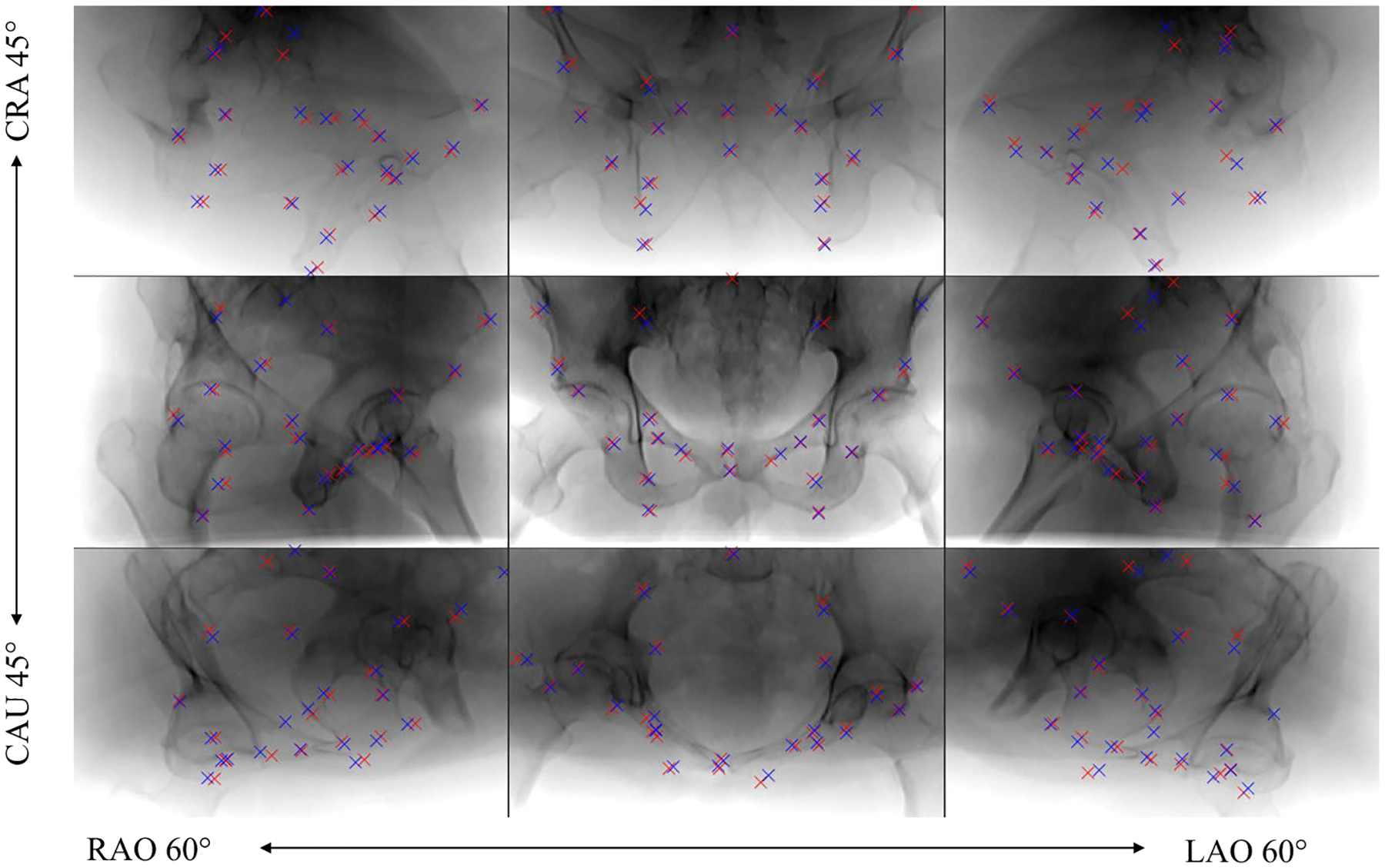
Predicted landmark positions for example projection images sampled across the sampled spherical segment of the synthetic test data set. Ground truth positions are marked with blue labels and automatic detection with red labels. Note that each projection image is processed independently

Fig. 4.

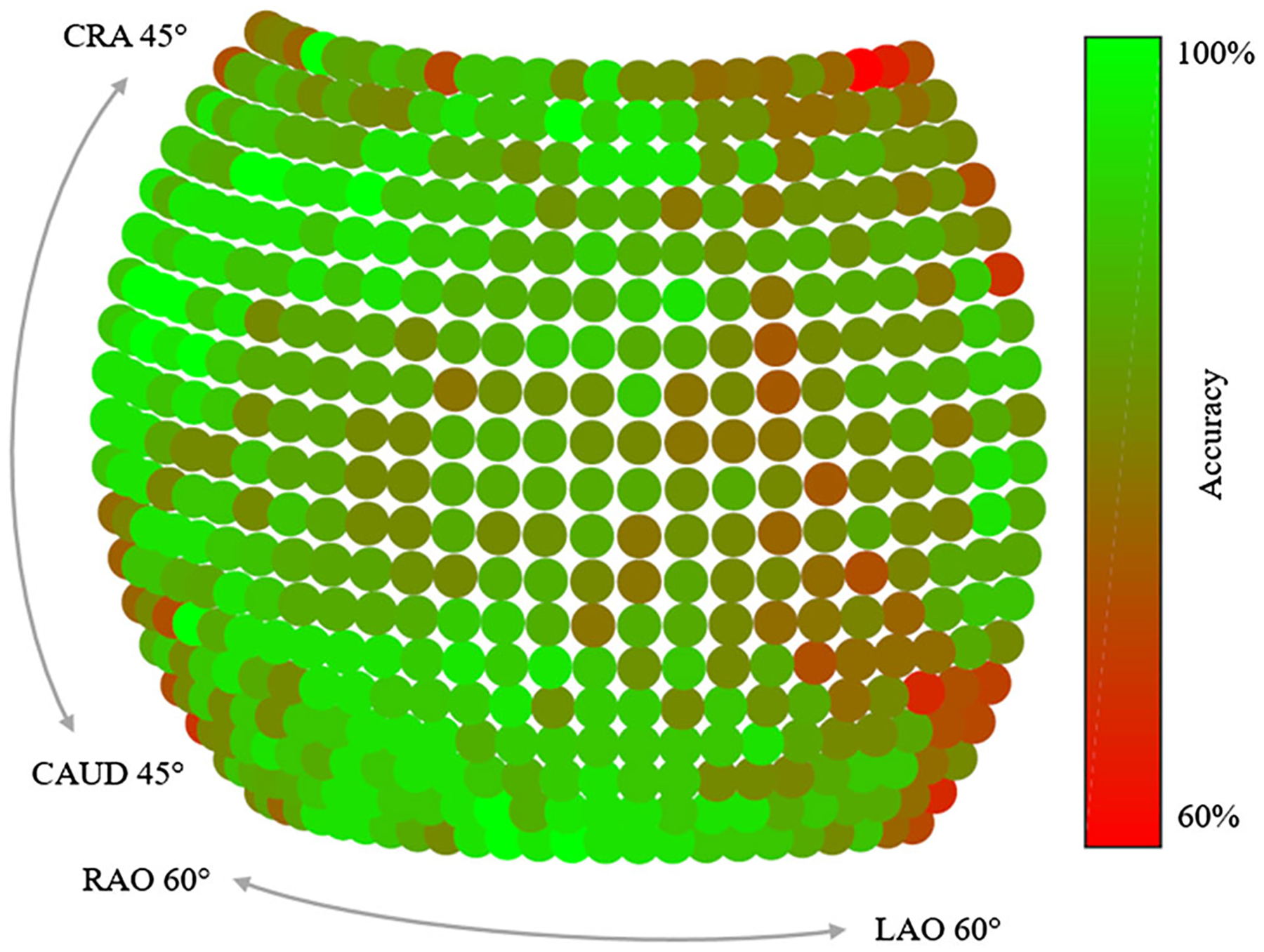
Accuracy depending on the viewing direction of the X-ray source. In average the detection result from central views is superior to the ones at the border of the sphere. The accuracy is defined as the ratio of landmarks that have an error below 15 pixels in the respective view

Fig. 8.

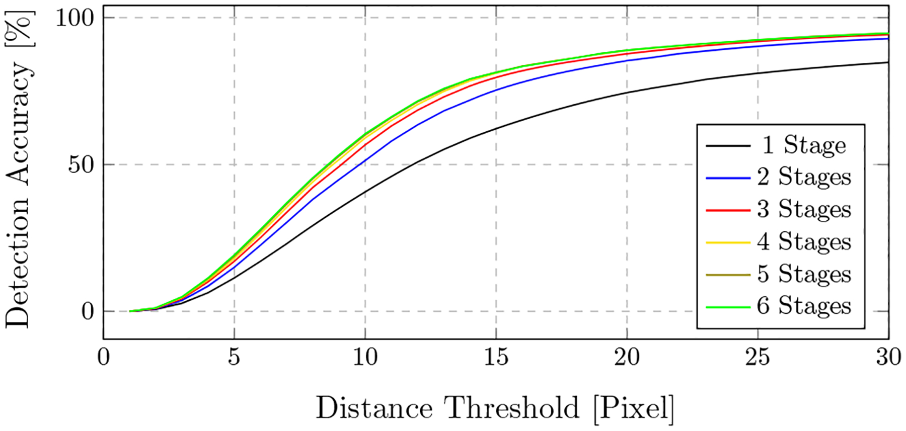
Accuracy depending on the distance threshold for intermediate stages

In Table 1, a more detailed analysis of the error across the different landmarks and the view position is presented. For each landmark, the average maximum belief, the average error across all projections, as well as the error across quadrants are shown. For the latter, the spherical segment is subdivided into four areas, centered at the AP position with two perpendicular divisions across the CRAN/CAUD and RAO/LAO axis. This reveals three interesting observations: First, some landmarks have an overall lower error (e.g., land mark #9 with an average error of 5.26pixels), while others are detected poorly (e.g., landmark #23 with an average error of 26.05pixels). Second, there exists a correlation between the average maximum belief response and the average error: The higher the response in a belief map, the lower the error. This observation is also supported by the scatter plot presented in Fig. 5, where for each prediction, the detection error is plotted over the corresponding maximum belief map response. Third, some landmarks can be detected equally well, independently of the viewing direction (e.g., landmark #11), while for others, the detectability highly varies across the quadrants (e.g., landmark #19). This observation is graphically well visible for these two landmarks, as shown in Fig. 6.

Table 1.

Individual landmark belief and error

Landmark #	Average belief	Average error (pixel)	Q1	Q2	Q3	Q4
1	0.79	7.60	9.42	5.35	7.13	7.89
2	0.84	6.68	5.66	7.67	6.63	6.05
3	0.83	6.86	9.13	7.81	5.07	5.26
4	0.87	7.69	8.79	10.2	7.11	4.70
5	0.85	7.53	8.11	8.47	6.63	6.62
6	0.82	5.63	4.72	5.21	5.97	6.35
7	0.78	7.90	7.96	7.48	8.29	7.99
8	0.77	10.1	5.87	12.1	7.70	15.3
9	0.90	5.26	5.15	5.08	5.55	5.07
10	0.88	7.19	7.60	6.90	5.80	8.41
11	0.89	6.43	5.77	5.99	6.86	6.83
12	0.91	7.78	8.96	7.23	5.71	8.55
13	0.92	4.47	5.64	4.10	4.67	3.24
14	0.90	5.64	3.70	7.00	5.24	6.18
15	0.85	9.04	8.77	9.54	7.75	10.3
16	0.82	7.23	6.55	6.95	7.26	8.18
17	0.81	19.9	20.0	24.2	15.2	21.1
18	0.80	15.3	11.2	16.6	14.5	19.3
19	0.74	9.56	10.4	10.4	9.80	7.09
20	0.77	8.59	5.78	12.9	6.83	8.91
21	0.51	9.40	14.3	6.86	13.9	8.51
22	0.44	13.7	9.73	25.0	10.1	16.2
23	0.51	26.0	24.2	17.6	39.3	29.8
Average	9.10 ± 7.38

Average Belief is the average of the highest responses in the belief maps for a certain landmark. Average Error is the average distance between the landmark detection and its ground truth location. The columns Q1, Q2, Q3 and Q4 also contain the average error, but evaluated only in a particular quadrant of the spherical segment to indicate detectability changes of certain landmarks across the spherical segment. Error values are given in pixels

Fig. 5.

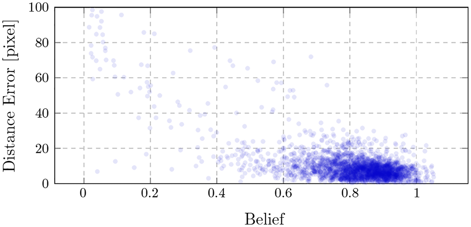
The error of a landmark detection is plotted onto the belief of the corresponding landmark detection. A correlation can be observed: Higher beliefs indicate lower detection errors

Fig. 6.

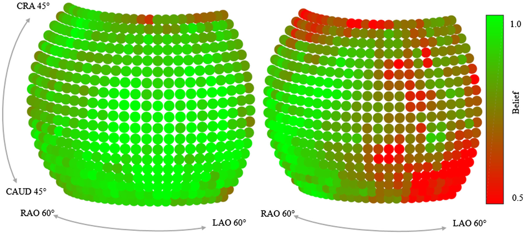
Maximum belief depending on the viewing direction for two landmarks (#11 and #19). While landmark #11 (left) is equally well visible across views, the belief for landmark #19 (right) changes substantially across views

We further investigated how the belief map response develops over the stages of the network and how ambiguities in the early stages are resolved. In Fig. 7, two example projections are shown, overlain by their corresponding belief maps at the respective stage. In the first row, the landmark of interest (tip of the right femoral head) is outside the field of view. However, a false position response appears after the first stage due to the similar appearance of the anatomy. With further stages, this ambiguity gets resolved. In the second row, a similar behavior is visible and a refinement of the prediction accuracy is clearly observable. The development of a landmark belief is also shown in Fig. 8. Here, the detection accuracy is plotted over the error distance tolerance for the belief maps at certain stages. Identical to above, a landmark is considered detected, if the error to its ground truth location is smaller than the Distance Threshold. It can be well observed that the detection results are refined with increasing stages.

Fig. 7.

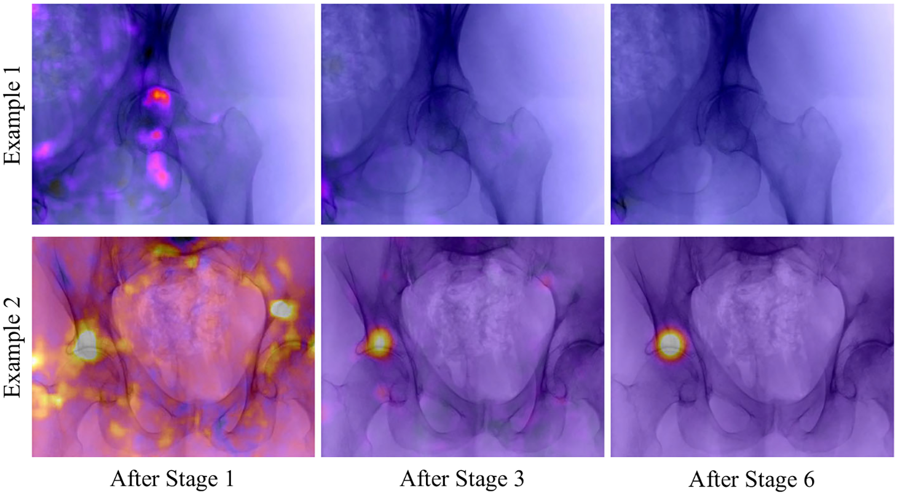
Initial, intermediate, and final belief map predicted by the model. The detection task in both cases is to detect the tip of the right femur. False positive responses due to ambiguities in the local image information are resolved over the stages

Clinical data

For the evaluation of the view-invariant landmark detection on real X-ray image data, five cadaveric data sets have been processed, each set consisting of a pre-operative CT scan and intra-operative X-ray sequences, taken from arbitrary and unknown viewing angles. In order to enable the retrieval of X-ray geometry, metal beads (BBs) were injected into the pelvis before imaging. To retrieve the X-ray projection geometry, first BB correspondences are established between individual images of the intra-operative X-ray sequence. Then, the fundamental matrix is computed for each image pair allowing for the 3D reconstruction of the BB positions [9]. This 3D reconstruction was then registered to the 3D BB locations extracted from the CT volume, allowing for an exact registration of each BB in 2D space to its corresponding location in 3D space. With these correspondences established, the projection matrices for each X-ray image were then calculated in closed form solution as in Eq. 2. To evaluate the reprojection error of these projection matrices (which defines a lower bound on the accuracy achievable using anatomical landmarks), the 3D BB coordinates as per the CT scan are forward projected into 2D space. Table 2 shows the reprojection error between the forward projection and the real X-ray images for the X-ray sequences. Note that one of this sequences has a tool in the field of view (sequence #3), while another shows a fracture of the pelvis (sequence #2). The low reprojection error of 2–5pixel is in line with our expectations and suggests that the resulting projection matrices are an appropriate reference when evaluating the performance of our proposed view-invariant landmark detection.

Table 2.

Quantitative evaluation for the detection results on the X-ray images of the cadaver specimens

Sequence	ref RPE	Landmark RPE	Landmark error
#1: specimen 1	2.45	74.31	120.9 (23.33 mm)
#2: specimen 1, with fracture	5.46	173.6	97.82 (18.87mm)
#3: specimen 1, with tool	2.88	177.4	63.67 (12.28 mm)
#4: specimen 2	2.86	119.4	127.9 (24.68 mm)
#5: specimen 2	2.99	115.3	79.89 (15.41mm)

Reprojection Errors (RPE) given in pixels. ref RPE is the error of the reference pose estimated from the metallic beads in order to project the 3D labels into the 2D X-ray images. Landmark RPE is the RPE of the metallic markers, using poses estimated with automatic anatomical landmark detections. Landmark Error is the distance of the detections to the ground truth positions. With a pixel size of 0.193mm/px, the metric error on the detector is given in mm

In the top row of Fig. 9, example landmark detection results in X-ray images of these sequences are shown. Automatic detections and ground truth locations are indicated with red and blue crosses, respectively. Overall, the well agreement between the automatic detections and the ground truth positions can be appreciated for various poses and truncations. In complicated situations when tools are present in the image, the landmark detection approach fails to detect the surrounding landmarks, as can be seen in example 4. However, this is not surprising since such situations were not part of the training data set. Small unknown objects, such as the metallic beads on the bone, seem to only have a limited influence on performance. Furthermore, example 5 depicts an image of the sequence where a fracture is present in the X-ray image, indicated with the white arrow. Qualitatively, this did not influence the detection substantially. Quantitatively, the overall deviation between true and predicted landmark locations averaged over the total 106 real images is shown in Table 2 in column titled Landmark Error.

Fig. 9.

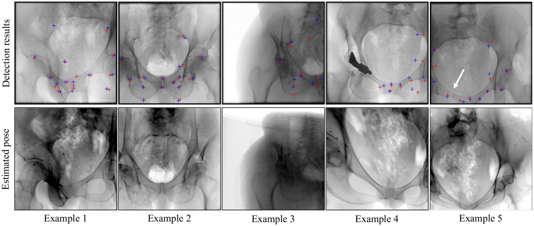
(Top) Detection results on clinical X-ray images. Landmark detection using the proposed approach is marked with a red cross, ground truth positions with a blue cross. (Bottom) Forward projections of the corresponding CT volume using the projection matrices computed by 2D/3D registration between the 2D landmark detections and the 3D labels in the CT volumes

The bottom row in Fig. 9 shows digitally reconstructed radiographs (DRRs) of the CT volumes belonging to the real X-ray image of the same patient shown above. The geometry for generating the DRRs has been obtained in closed form 2D/3D registration of the detected landmarks to the 3D labels in the CT volume, as described in “2D/3D registration” section. For these various poses, the landmark detection accuracy proves sufficient to achieve views that are very similar to the target X-ray image, suggesting successful initialization.

Discussion and conclusion

We presented a novel approach to detect anatomical landmarks in X-ray images independent of the viewing direction. The landmark locations supply additional information for the surgeon and enable various applications, including global initialization of 2D/3D registration in closed form. Due to the characteristics of transmission imaging, landmark appearances change substantially with the viewing direction making anatomical landmark detection a challenging task that has, to the best of our knowledge, not previously been addressed.

We employed a convolutional neural network that consists of multiple stages. Given a single input image, multiple belief maps are inferred and refined based on local image information and belief maps of the preceding stage, finally indicating the respective landmark location. The network was trained on synthetic data generated using a physics-based framework and evaluated on both synthetic and real test sets, revealing promising performance.

Despite encouraging results, some limitations remain that we discuss in the following paragraph, pointing to possible future research directions to overcome or alleviate these. First of all, the robustness toward unseen scenarios such as tools in the image or changes of the anatomy due to fractured anatomy must be improved. This issue could be addressed with a larger data set that contains such variation. Also, the accuracy from views of the border of the spherical segment is slightly inferior compared to frontal views. This might be explained by the higher amount of overlapping anatomy from these directions as well as a lower amount of variation of the training data sampled in this area. A possible solution could be to increase the angular range during training, while limiting validation to the current range Further, the network architecture in its current state yields belief maps that are downsampled by a factor of around eight compared to the input image. This downsampling inherently limits the accuracy of the detection results. While this accuracy may have been sufficient for the initial purpose of human pose estimation, in medical imaging, higher accuracy is desirable. Possible improvements that are subject to future work could be achieved by competing network architectures based on an encoder–decoder design with skip connections in order to preserve resolution of the output images. Alternatively, test-time augmentation could be applied by processing slightly altered versions of the input image with the same network during application. The results of these multiple outputs could subsequently be averaged, which might yield higher accuracy. Furthermore, the robustness as well as the overall accuracy could benefit by providing prior knowledge in the form of a model-based post-processing step. A possible source of error might be introduced by the labeling of the landmarks in the 3D volume that, since manual, is inherently prone to errors. Ideally, an unsupervised landmark or keypoint selection process would be of great benefit for this approach. As a possible application, we showed that an initialization of 2D/3D registration based on the automatic detections is successful without the need for additional calibration. In this work, we relied on a closed form solution to estimate the image pose which is compelling due to its simplicity, yet a more sophisticated approach based on maximum likelihood would certainly yield superior results in the presence of statistical outliers. In this task, we also showed that considering the maximum belief is powerful for selecting reliably detected landmarks. This additional information can be used as a confidence measure for further processing tasks. Recently, the proposed concept of view-invariant anatomical landmark detection has been transferred to projection images of knees in an attempt to estimate involuntary motion during scans [3].

In conclusion, detecting anatomical landmarks has grown to be an essential tool in automatic image parsing in diagnostic imaging, suggesting similar importance for image-guided interventions. The implementation of anatomical landmarks as a powerful concept for aiding image-guided interventions will be pushed continuously as new approaches, such as this one, strive to achieve clinically acceptable performance.

References

- 1.Aichert A, Berger M, Wang J, Maass N, Doerfler A, Hornegger J, Maier AK (2015) Epipolar consistency in transmission imaging. IEEE Trans Med Image 34(11):2205–2219 [DOI] [PubMed] [Google Scholar]
- 2.Baumgartner R, Libuit K, Ren D, Bakr O, Singh N, Kandemir U, Marmor MT, Morshed S (2016) Reduction of radiation exposure from c-arm fluoroscopy during orthopaedic trauma operations with introduction of real-time dosimetry. J Orthop Trauma 3(2):e53–e58 [DOI] [PubMed] [Google Scholar]
- 3.Bier B, Aschoff K, Syben C, Unberath M, Levenston M, Gold G, Fahrig R, Maier A (2018) Detecting anatomical landmarks for motion estimation in weight-bearing imaging of knees In: International workshop on machine learning for medical image reconstruction. Springer, New York, pp 83–90 [Google Scholar]
- 4.Bier B, Unberath M, Zaech JN, Fotouhi J, Armand M, Osgood G, Navab N, Maier A (2018) X-ray-transform invariant anatomical landmark detection for pelvic trauma surgery. In: International conference on medical image computing and computer-assisted intervention Springer, New York, pp 55–63 [Google Scholar]
- 5.Fedorov A, Beichel R, Kalpathy-Cramer J, Finet J, Fillion-Robin JC, Pujol S, Bauer C, Jennings D, Fennessy F, Sonka M, Buatti J, Aylward S, Miller J, Pieper S, Kikinis R (2012) 3d slicer as an image computing platform for the quantitative imaging network. Magn Reson Imaging 30(9):1323–1341 [DOI] [PMC free article] [PubMed] [Google Scholar]
- 6.Ghesu FC, Georgescu B, Mansi T, Neumann D, Hornegger J, Comaniciu D (2016) An artificial agent for anatomical landmark detection in medical images In: MICCAI. Springer, New York, pp 229–237 [Google Scholar]
- 7.Ghesu FC, Georgescu B, Zheng Y, Grbic S, Maier A, Hornegger J, Comaniciu D (2017) Multi-scale deep reinforcement learning for real-time 3d-landmark detection in ct scans. IEEE Trans Pattern Anal Mach Intell 41:176–189 [DOI] [PubMed] [Google Scholar]
- 8.Härtl R, Lam KS, Wang J, Korge A, Audigé FKL (2013) Worldwide survey on the use of navigation in spine surgery. World Neurosurg 379(1):162–172 [DOI] [PubMed] [Google Scholar]
- 9.Hartley RI, Zisserman A (2004) Multiple view geometry in computer vision. Cambridge University Press, Cambridge: ISBN 0521540518 [Google Scholar]
- 10.Heimann T, Meinzer HP (2009) Statistical shape models for 3d medical image segmentation: a review. Med Image Anal 13(4):543–563 [DOI] [PubMed] [Google Scholar]
- 11.Hou B, Alansary A, McDonagh S, Davidson A, Rutherford M, Hajnal JV, Rueckert D, Glocker B, Kainz B (2017) Predicting slice-to-volume transformation in presence of arbitrary subject motion In: MICCAI. Springer, New York, pp 296–304 [Google Scholar]
- 12.Johnson HJ, Christensen GE (2002) Consistent landmark and intensity-based image registration. IEEE Trans Med Imaging 21(5):450–461 [DOI] [PubMed] [Google Scholar]
- 13.Khurana B, Sheehan SE, Sodickson AD, Weaver MJ (2014) Pelvic ring fractures: what the orthopedic surgeon wants to know. Radio-graphics 34(5):1317–1333 [DOI] [PubMed] [Google Scholar]
- 14.Litjens G, Kooi T, Bejnordi BE, Setio AAA, Ciompi F, Ghafoorian M, van der Laak JA, Van Ginneken B, Sánchez CI (2017) A survey on deep learning in medical image analysis. Med Image Anal 42:60–88 [DOI] [PubMed] [Google Scholar]
- 15.Liu D, Zhou KS, Bernhardt D, Comaniciu D (2010) Search strategies for multiple landmark detection by submodular maximization. In: 2010 IEEE conference on computer vision and pattern recognition (CVPR), IEEE, pp 2831–2838 [Google Scholar]
- 16.Mader AO, von Berg J, Fabritz A, Lorenz C, Meyer C (2018) Localization and labeling of posterior ribs in chest radiographs using a CRF-regularized FCN with local refinement. In: International conference on medical image computing and computer-assisted intervention Springer, New York, pp 562–570 [Google Scholar]
- 17.Markelj P, Tomaževič D, Likar B, Pernuš F (2012) A review of 3d/2d registration methods for image-guided interventions. Med Image Anal 16(3):642–661 [DOI] [PubMed] [Google Scholar]
- 18.Payer C, Štern D, Bischof H, Urschler M (2016) Regressing heatmaps for multiple landmark localization using CNNS. In: International conference on medical image computing and computer-assisted intervention Springer, New York, pp 230–238 [Google Scholar]
- 19.Pouch AM, Yushkevich PA, Jackson BM, Jassar AS, Vergnat M, Gorman JH, Gorman RC, Sehgal CM (2012) Development of a semi-automated method for mitral valve modeling with medial axis representation using 3d ultrasound. Med Phys 39(2):933–950 [DOI] [PMC free article] [PubMed] [Google Scholar]
- 20.Roth H, Lu L, Seff A, Cherry KM, Hoffman J, Wang S, Summers RM (2015) A new 2.5 D representation for lymph node detection in CT. Cancer Imaging Arch. 10.7937/K9/TCIA.2015.AQIIDCNM [DOI] [Google Scholar]
- 21.Sa R, Owens W, Wiegand R, Studin M, Capoferri D, Barooha K, Greaux A, Rattray R, Hutton A, Cintineo J, Chaudhary V (2017) Intervertebral disc detection in x-ray images using faster r-cnn. In: 2017 39th annual international conference of the IEEE engineering in medicine and biology society (EMBC), IEEE, pp 564–567 [DOI] [PubMed] [Google Scholar]
- 22.Starr R, Jones A, Reinert C, Borer D (2001) Preliminary results and complications following limited open reduction and percutaneous screw fixation of displaced fractures of the acetabulum. Injury 32:SA45–SA50 [DOI] [PubMed] [Google Scholar]
- 23.Štern D, Ebner T, Urschler M (2016) From local to global random regression forests: exploring anatomical landmark localization. In: International conference on medical image computing and computer-assisted intervention Springer, New York, pp 221–229 [Google Scholar]
- 24.Stöckle U, Schaser K, König B (2007) Image guidance in pelvic and acetabular surgery-expectations, success and limitations. Injury 38(4):450–462 [DOI] [PubMed] [Google Scholar]
- 25.Tucker E, Fotouhi J, Unberath M, Lee SC, Fuerst B, Johnson A, Armand M,Osgood GM, Navab N (2018) Towards clinical translation of augmented orthopedic surgery: from pre-op CT to intra-op x-ray via RGBD sensing In: Medical imaging 2018: imaging informatics for healthcare, research, and applications, vol 10579 International Society for Optics and Photonics, p 105790J [Google Scholar]
- 26.Unberath M, Zaech JN, Lee SC, Bier B, Fotouhi J, Armand M, Navab N (2018) Deepdrr–a catalyst for machine learning in fluoroscopy-guided procedures. In: International conference on medical image computing and computer-assisted intervention Springer, New York [Google Scholar]
- 27.Urschler M, Ebner T, Štern D (2018) Integrating geometric configuration and appearance information into a unified framework for anatomical landmark localization. Med Image Anal 43:23–36 [DOI] [PubMed] [Google Scholar]
- 28.Wang CW, Huang CT, Hsieh MC, Li CH, Chang SW, Li WC, Vandaele R, Marée R, Jodogne S, Geurts P, Chen C, Zhen G, Chu C, Mirzaalian H, Vrtovec T, Ibragimov B (2015) Evaluation and comparison of anatomical landmark detection methods for cephalometric x-ray images: a grand challenge. IEEE Trans Med Imaging 34(9):1890–1900 [DOI] [PubMed] [Google Scholar]
- 29.Wei SE, Ramakrishna V, Kanade T, Sheikh Y (2016) Convolutional pose machines In: CVPR, pp 4724–4732 [Google Scholar]
- 30.Xie W, Franke J, Chen C, Grützner PA, Schumann S, Nolte LP, Zheng G (2015) A complete-pelvis segmentation framework for image-free total hip arthroplasty (tha): methodology and clinical study. Int J Med Robot Comput Assist Surg 11(2):166–180 [DOI] [PubMed] [Google Scholar]
- 31.Zheng Y, Barbu A, Georgescu B, Scheuering M, Comaniciu D (2008) Four-chamber heart modeling and automatic segmentation for 3-d cardiac ct volumes using marginal space learning and steerable features. IEEE Trans Med Imaging 27(11):1668–1681 [DOI] [PubMed] [Google Scholar]