Statistical properties of cerebral CT perfusion imaging systems. Part I. Cerebral blood volume maps generated from nondeconvolution-based systems

Abstract

Purpose:

The development and clinical employment of a computed tomography (CT) imaging system benefit from a thorough understanding of the statistical properties of the output images; cerebral CT perfusion (CTP) imaging system is no exception. A series of articles will present statistical properties of CTP systems and the dependence of these properties on system parameters. This Part I paper focuses on the signal and noise properties of cerebral blood volume (CBV) maps calculated using a nondeconvolution-based method.

Methods:

The CBV imaging chain was decomposed into a cascade of subimaging stages, which facilitated the derivation of analytical models for the probability density function, mean value, and noise variance of CBV. These models directly take CTP source image acquisition, reconstruction, and postprocessing parameters as inputs. Both numerical simulations and in vivo canine experiments were performed to validate these models.

Results:

The noise variance of CBV is linearly related to the noise variance of source images and is strongly influenced by the noise variance of the baseline images. Uniformly partitioning the total radiation dose budget across all time frames was found to be suboptimal, and an optimal dose partition method was derived to minimize CBV noise. Results of the numerical simulation and animal studies validated the derived statistical properties of CBV.

Conclusions:

The statistical properties of CBV imaging systems can be accurately modeled by extending the linear CT systems theory. Based on the statistical model, several key signal and noise characteristics of CBV were identified and an optimal dose partition method was developed to improve the image quality of CBV.

1. INTRODUCTION

Cerebral computed tomography perfusion (CTP) is an imaging technique to assess the blood perfusion status of brain parenchyma. The technique involves rapid sequential CT scans of the head following intravenous administration of an iodinated contrast bolus. Based on certain tracer kinetics models, the acquired contrast-enhanced and time-resolved CT images are processed by either deconvolution- or nondecovolution-based algorithms to generate maps of parametric perfusion parameters such as cerebral blood volume (CBV) and cerebral blood flow (CBF). The concept of this imaging technique was initially proposed in 1980 by Axel.¹ Later in 1991, Miles et al. developed a practical method to display information extracted from CTP imaging by means of color maps.² These pioneering works, together with the improved accuracy and acquisition speed resulting from the advent of multidetector row CT (MDCT), has stimulated more frequent clinical use of CTP in the diagnosis and management of acute ischemic stroke (AIS),^3–8 transient ischemic stroke,^9–12 stroke mimics,¹³ aneurysmal subarachnoid hemorrhage,^14–16 ischemic Moyamoya disease,^17,18 and other neurological diseases.¹⁹ Among these applications, the use of CTP for selecting AIS patients for endovascular therapy has drawn particular attention. Multiple clinical trials demonstrated potential benefits of using CTP to select patients most likely to benefit from endovascular therapy and exclude one for whom the therapy may carry higher risk of further injury.^8,20–22

Despite the broad scope of CTP’s clinical applications, the reliability of perfusion information extracted from parametric CTP maps remains somewhat controversial.^23–27 One of the major technical reasons is the distinct lack of standardization for the acquisition, reconstruction, and postprocessing methods across vendors and institutions, which often leads to substantial variability in the measured tissue perfusion information.^28–33 The reliability of CTP imaging is also severely impeded by its limited quantification accuracy and low signal-to-noise ratio (SNR),^24,34 despite its requirement for relatively high radiation exposure.^35–37 Due to these technical limitations, there is strong call from the clinical neuroimaging community to “improve the science (of CTP) before changing clinical practice.”²⁶

In order to improve the science of an imaging technology, the science must be thoroughly understood in the first place. This rationale has been instrumental in advancing not only CTP but also the whole CT field. However, when the subject of CTP imaging science is reviewed, there is a major missing piece about how statistical properties of the system outputs (parametric perfusion maps) depend on the system inputs. This piece of information is important since it directly determines the quantification accuracy (bias) and precision of perfusion maps. Achieving this understanding is quite challenging: unlike other CT applications that directly generate interpretable images after tomographic reconstruction, CTP requires an extra postprocessing step, in which the temporal dimension is removed from the dynamic images using operations such as deconvolution and the extraction of a maximum value. These operations are not directly covered in the classical linear CT systems theory, and thus the properties of signal and noise transferred through these operations cannot be analyzed by borrowing the existing knowledge. Consequently, a clear understanding on the quantitative relationship between CTP imaging performance and input parameters is lacking. Selection of these parameters is often performed ad hoc — namely, heavily relying on developers’ experience, clinicians’ feedback, and other empirical findings. No scientific guiding principle is available to allow a synergistic optimization of the whole CTP imaging chain to generate the most reliable imaging outcome.

In a series of papers, we report our theoretical studies on the statistical properties of CTP imaging systems. The ultimate goal was to advance knowledge and improve reliability of the CTP technology. The direct goal was to establish a theoretical framework covering the quantitative relationship between signal and noise properties of perfusion maps and system input parameters. Cascaded systems analysis was applied and classical linear CT systems theory was extended to cover deconvolution and maximum operators encountered in CTP imaging.

In this Part I paper, we focused on the statistical properties of CBV map generated from nondeconvolution (aka direct method)-based CTP imaging systems. As shown later in Eq. (1), CBV produced from these systems does not involve the use of deconvolution or the maximum operator, and thus its signal and noise properties can be analyzed quite straightforwardly. We use this topic to jump-start subsequent analysis of more complex deconvolution-based systems. Some preliminary results on the noise properties of nondeconvolution-based CBV systems were reported in our conference proceeding.³⁸ The current paper presents additional statistical properties of CBV such as its mean value and probability density function, provides scientific evidences to justify underlying assumptions of the theoretical deviation, and reports additional quantitative results to validate the theory.

2. CASCADED SYSTEMS ANALYSIS

2.A. Signal model of CBV

CBV quantifies the volume of blood contained in the capillary bed within a unit mass of brain tissue. Intracranial hematoma or acute cerebral hemorrhage may result in a “erroneous” increase in CBV since blood is no longer confined in the capillary bed. In comparison, ischemic strokes may result in a significant reduction in CBV. For example, previous studies have shown that severely reduced CBV could be a strong predictor of hemorrhagic transformation and functional outcomes following endovascular therapy for AISs.^5,6

CBV can be estimated from the integrals of time-iodine density curves measured at an artery (C_artery) and brain tissue (C_tissue) as follows^39,40

$$\text{CBV}(\overrightarrow{x})=\kappa \frac{\int C_{\text{tissue }}(\overrightarrow{x},t)\text{d}t}{\int C_{\text{artery }}(t)\text{d}t},$$ (1)

where κ is a numerical factor determined by the density of brain tissue (ρ) and hematocrit ratio (H) between artery and capillary bed within brain tissue as follows:

$$\kappa =\frac{H}{\rho }.$$ (2)

In CTP imaging, both arterial and tissue time-density curves are estimated from time-resolved CT images, referred to as CTP source images or $I(\overrightarrow{x},t)$ in this work. The enhancement in CT numbers caused by the iodinated contrast medium is assumed to be linearly proportional to the iodine density,² namely

$$C_{\text{tissue }}(\overrightarrow{x},t)=\alpha \left[I(\overrightarrow{x},t)-I_b(\overrightarrow{x})\right],$$ (3)

where $I_b(\overrightarrow{x})$ is a “baseline” or “mask” image acquired before the wash-in of iodinated contrast, and α is a numerical scaling factor. Likewise, the time-density curve of the artery, namely the arterial input function (AIF), can be measured at spatial location ${\overrightarrow{x}}_0$ that corresponds to a major feeding cerebral artery as

$$C_{\text{artery }}(t)=\alpha \left[I\left({\overrightarrow{x}}_0,t\right)-I_b\left({\overrightarrow{x}}_0\right)\right].$$ (4)

As a result, CBV is related to the pixel value of CTP source images as

$$\text{CBV}(\overrightarrow{x})=\kappa \frac{{\int }_0^T\left[I(\overrightarrow{x},t)-I_b(\overrightarrow{x})\right]\text{d}t}{{\int }_0^T\left[I\left({\overrightarrow{x}}_0,t\right)-I_b\left({\overrightarrow{x}}_0\right)\right]\text{d}t},$$ (5)

where T is the total CT image acquisition time.

For the precontrast baseline image $I_b(\overrightarrow{x})$ in Eq. (5), it is often obtained by averaging multiple time frames acquired prior to contrast arrival in order to reduce noise:

$$I_b(\overrightarrow{x})=\frac{1}{T_b}{\int }_0^{T_b}I(\overrightarrow{x},t)\text{d}t.$$ (6)

Based on Eq. (6), the integration limits in Eq. (5) can be shrunk from [0,T] to [T_b, T], because

$${\int }_0^{T_b}\left[I(\overrightarrow{x},t)-I_b(\overrightarrow{x})\right]\text{d}t={\int }_0^{T_b}I(\overrightarrow{x},t)\text{d}t-T_b{I}_b(\overrightarrow{x})\equiv 0.$$ (7)

In other words, the formula of CBV in Eq. (5) can be rewritten as

$$\begin{gathered} \text{CBV}(\overrightarrow{x})=\kappa \frac{{\int }_{T_b}^T\left[I(\overrightarrow{x},t)-I_b(\overrightarrow{x})\right]\text{d}t}{{\int }_{T_b}^T\left[I\left({\overrightarrow{x}}_0,t\right)-I_b\left({\overrightarrow{x}}_0\right)\right]\text{d}t} \\ =\kappa \frac{A(\overrightarrow{x})}{B}, \end{gathered}$$ (8)

where A denote the area under the tissue enhancement curve, and B denotes the area under the AIF.

Based on Eq. (8), the expected value of CBV, denoted as $\overline{\text{CBV}}$, is related to the expected value of CTP source images by

$$\begin{gathered} \overline{\text{CBV}}(\overrightarrow{x})=\kappa \frac{\overline{A}(\overrightarrow{x})}{\overline{B}} \\ =\kappa \frac{{\int }_{T_b}^T\left[\overline{I}(\overrightarrow{x},t)-{\overline{I}}_b(\overrightarrow{x})\right]\text{d}t}{{\int }_{T_b}^T\left[\overline{I}\left({\overrightarrow{x}}_0,t\right)-{\overline{I}}_b\left({\overrightarrow{x}}_0\right)\right]\text{d}t}. \end{gathered}$$ (9)

In practice, an additional numerical scaling factor may be applied to the measured AIF to compensate for the magnitude drop associated with the partial volume effect (PVE).

2.B. Noise model of CBV

Due to the presence of noise in the measured CTP source images, a single measurement of CBV is likely to deviate from the expected value by a stochastic amount of ΔCBV:

$$\overline{\text{CBV}}(\overrightarrow{x})=\overline{\text{CBV}}(\overrightarrow{x})+\Delta \text{CBV}(\overrightarrow{x}).$$ (10)

By definition, the expected value of the square of ΔCBV is the noise variance of CBV:

$${\sigma }_{\text{CBV}}^2(\overrightarrow{x})=\overline{{\Delta }^2\text{CBV}(\overrightarrow{x})}.$$ (11)

As shown in Appendix 1, ${\sigma }_{\text{CBV}}^2(\overrightarrow{x})$ is related to the noise variance of the source image $({\sigma }_{\text{0}}^2)$ by

$$\begin{gathered} {\sigma }_{\text{CBV}}^2(\overrightarrow{x})\approx {\left(\frac{\kappa \Delta t}{\overline{B}}\right)}^2\left[\left(N-N_b\right){\sigma }_0^2(\overrightarrow{x})+{\left(N-N_b\right)}^2{\sigma }_b^2(\overrightarrow{x})\right] \\ ={\left(\frac{\kappa \Delta t}{\overline{B}}\right)}^2\left[N_a{\sigma }_0^2(\overrightarrow{x})+N_a^2{\sigma }_b^2(\overrightarrow{x})\right], \end{gathered}$$ (12)

where N = T/Δt is the total number of time frames, N_b is the number of baseline time frames, N_a = N − N_b the number of nonbaseline time frames. Since $N_a^2\gg N_a$, the noise of CBV has a much stronger dependence on the baseline image noise $({\sigma }_b^2)$.

When deriving Eq. (12), it was assumed that the noise of CTP source image is stationary and uncorrelated along the temporal dimension. An experimental validation of this assumption is presented in Fig. 1. The autocovariance matrix shown in this figure was measured in a relatively uniform 70 mm² region (ventricle) in the CTP source images acquired from a diagnostic MDCT system (GE Discovery CT750 HD). Note that although certain time frames may experience larger x-ray attenuation due to higher iodine enhancement, the absolute enhancement is usually 1% or 2% (10–20 HU) for majority of the brain tissues, thus the overall dependence of ${\sigma }_0^2$ on time is weak.

FIG. 1.

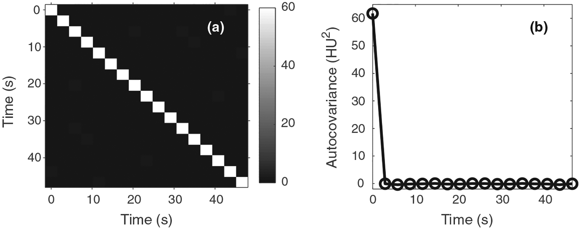
(a) Autocovariance matrix measured along the temporal direction from experimental computed tomography perfusion source images. (b) Plot of the first column of the autocovariance matrix. These results demonstrate that noise in the source images is approximately stationary and uncorrelated along the temporal direction.

Regarding the statistical distribution function of CBV, if the pixel value of each source image frame can be considered as a normally distributed random variable, based on the general properties of the normal distribution, CBV is distributed normally and its probability density function can be uniquely from $\overline{\text{CBV}}$ in Eq. (9) and ${\sigma }_{\text{CBV}}^2$ in Eq. (12):

$$\text{CBV}(\overrightarrow{x})~\mathcal{N}\left[\overline{\text{CBV}}(\overrightarrow{x}),{\sigma }_{\text{CBV}}^2(\overrightarrow{x})\right].$$ (13)

2.C. Example application of the theoretical model: Optimal dose partition

As indicated by Eq. (12), an effective approach to reduce CBV noise is to reduce noise of the baseline images, which can be achieved by increasing radiation exposure for the baseline frames. Since the total radiation dose D delivered during a CTP exam cannot be arbitrarily increased, an interesting question is: how to optimally partition D to the baseline and nonbaseline frames during a CTP exam in order to minmize CBV noise?

To help answer this question, the following well-known relationship between CT noise and radiation dose is utilized:

$$\begin{gathered} {\sigma }_0^2(\overrightarrow{x})\propto \frac{1}{D_a} \\ =\frac{\beta (\overrightarrow{x})}{D_a}, \end{gathered}$$ (14)

where D_a denotes radiation dose delivered to each nonbaseline frame, β denotes a numerical scaling factor that depends on the image object, reconstruction method, and postrecon-struction image smoothing kernel. For the baseline image I_b, since it is averaged from N_b image frames, its noise variance is related to the dose per baseline frame (D_b) by:

$${\sigma }_b^2(\overrightarrow{x})=\frac{1}{N_b}\frac{\beta (\overrightarrow{x})}{D_b},$$ (15)

Correspondingly, noise variance of CBV can be expressed in terms of D_a and D_b as

$$\begin{gathered} {\sigma }_{\text{CBV}}^2(\overrightarrow{x})={\left(\frac{\kappa \Delta t}{\overline{B}}\right)}^2\left(\frac{N_a\beta (\overrightarrow{x})}{D_b}+\frac{N_a^2\beta (\overrightarrow{x})}{N_b{D}_b}\right) \\ ={\left(\frac{\kappa \Delta t{N}_a}{\overline{B}}\right)}^2\beta (\overrightarrow{x})\left(\frac{1}{N_a{D}_a}+\frac{1}{N_b{D}_b}\right) \\ \propto \left(\frac{1}{N_a{D}_a}+\frac{1}{N_b{D}_b}\right). \end{gathered}$$ (16)

Based on Eq. (16), the optimal dose partition problem can be formulated as the following constrained optimization problem:

$$\left\{D_a^{*},D_b^{*}\right\}=\underset{D_a,D_b}{\text{arg}\text{min}}\left[\frac{1}{N_a{D}_a}+\frac{1}{N_b{D}_b}\right],$$ (17)

subject to

$$D=N_b{D}_b^{*}+N_a{D}_a^{*}.$$ (18)

Solution of this constrained optimization problem is given by (Appendix II)

$$D_b^{*}=\frac{D}{2N_b},D_a^{*}=\frac{D}{2N_a}.$$ (19)

In other words, the total dose delivered to the N_b baseline frames is equal to the total dose delivered to all the nonbaseline frames:

$$N_b{D}_b^{*}=N_a{D}_a^{*}=\frac{D}{2}.$$ (20)

The ratio in dose rate between baseline and nonbaseline frames is

$$\frac{D_b^{*}}{D_a^{*}}=\frac{N_a}{N_b}=\frac{N-N_b}{N_b}.$$ (21)

Since N_a is usually much larger than N_b, Eq. (21) indicates that a larger exposure rate should be used for baseline frames than subsequent nonbaseline frames.

In comparison, most clinical CTP scan protocols use a uniform dose partitioning strategy, namely:

$$D_a=D_b=\frac{D}{N}.$$ (22)

Based on Eqs. (16), (20), and (22), the ratio in ${\sigma }_{\text{CBV}}^2$ between the optimized and uniform dose partition method is:

$$\frac{{{\sigma }_{\text{CBV}}^2|}_{\text{opt}}}{{{\sigma }_{\text{CBV}}^2|}_{\text{uniform }}}=\frac{4\left(N-N_b\right)N_b}{N^2}.$$ (23)

This ratio is always ≤1, since

$$4\left(N-N_b\right)N_b-N^2=-{\left(N-2N_b\right)}^2\le 0.$$ (24)

Except in the rare case where N_b = N/2, the optimal dose partition method leads to lower CBV noise. In practice, the most straight forward approach to implement the optimized dose partitioning scheme is to modulate tube current (mA) as a function of time frame. However, some vendors do not allow the tube current to be modulated during a sequential scan mode (aka cine mode). Certain scanner models may offer a changeable temporal sampling interval, which allows N_b to be increased. Based on Eq. (20), if N_b = N_a, the optimal condition can still be met without modulating the mA. This is similar to what has been widely used in digital subtraction angiography (DSA) imaging, where a high number of baseline frames is quickly acquired in order to reduce baseline image noise and improve the final DSA image quality.

3. VALIDATION METHODS

3.A. Numerical simulations

To validated the signal and noise model, an anthropomorphic 4D digital CTP phantom^41,42 was used. As shown in Fig. 2(a), the phantom simulates the anatomy of human brain based on a clinical MRI dataset. Models of the skull, vessels and ventricles were included in this digital phantom (Fig. 2). In the brain parenchyma, regions with reduced and severely reduced blood flow were created. The ground truth for the perfusion properties of different brain tissues is listed in Table I. Ground truth for the AIF is shown in Fig. 2(b). The value of κ in Eq. (1) was assumed to be 1.0 [mL/g].

FIG. 2.

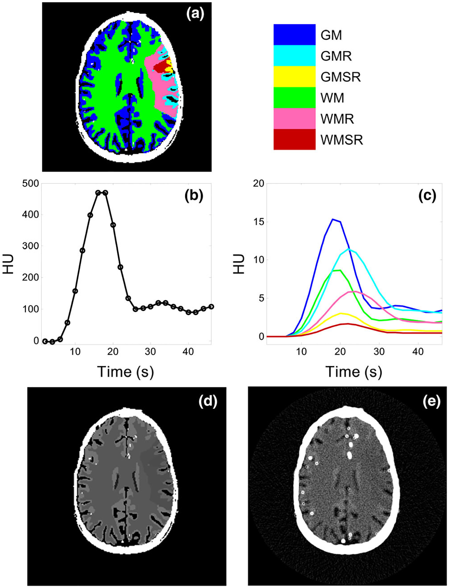
Digital head phantom used in the simulation study (a) Tissue types and locations. (b) Ground truth of the arterial input function. (c) Ground truth of the tissue enhancement curves. (d) Ground truth of the source image at the 9th time frame. (e) A noisy realization of the source image. Blooming of vessels and skull was due to the finite spatial resolution of the simulated CT system. The color legend applies to both (a) and (c). The display window/level in (d) and (e) are 100/50 HU.

Table I.

Ground truth for the cerebral blood volume (in ml/100 g) and CBF (in ml/100 g/min) used in the numerical simulations.

Tissue type	Abbreviation	CBV	CBF
Grey matter	GM	3.3	53
Grey matter with reduced flow	GMR	2.9	16
Grey matter with severely reduced flow	GMSR	0.7	5.3
White matter	WM	1.9	25
White matter with reduced flow	WMR	1.6	7.5
White matter with severely reduced flow	WMSR	0.4	2.5

Based on the true CBV and CBF values listed in Table I, a so-called flow-scaled residue function⁴⁰ was constructed for each spatial location $\overrightarrow{x}$ in the brain tissue:

$$R(\overrightarrow{x},t)=\{\begin{array}{cc}\rho \cdot \text{CBF}(\overrightarrow{x})& \text{ if }t\le t_0;\\ \rho \cdot \text{CBF}(\overrightarrow{x}){\text{e}}^{-\frac{t-t_0(\overrightarrow{x})}{\tau }}& \text{ if }t>t_0,\end{array}$$ (25)

where constant τ=1 s, tissue mass density ρ=1 g/ml, and t₀ is jointly determined by CBV and CBF as

$$t_0(\overrightarrow{x})=\frac{\text{CBV}(\overrightarrow{x})}{\text{CBF}(\overrightarrow{x})}-\tau .$$ (26)

For each tissue type, a convolution of its flow-scaled residue function in Eq. (25) with the true AIF provided its true tissue enhancement curve shown in Fig. 2(c).

In order to simulate noisy CTP source images of this digital phantom, each time frame of the original noise-free phantom image were forward-projected along 1000 angular directions uniformly distributed over an angular span of 360°. Poisson noise was added to the simulated prelog projection data. To model noise correlations imposed by the CT acquisition system, the noisy projection data were filtered by a Gaussian kernel, which enabled the texture of the CTP source images to closely resemble that of experimental CT images. Noisy CTP source images were reconstructed from the noisy projection data using filtered backprojection, and CBV maps were calculated from these source images using Eq. (8). For each CTP acquisition protocol, the simulation process was repeated 510 times to generate an ensemble of CBV maps, from which ${\sigma }_{\text{CBV}}(\overrightarrow{x})$ and $\overline{\text{CBV}}(\overrightarrow{x})$ can be measured at any spatial location $(\overrightarrow{x})$ in the phantom.

The simulations were performed with the following image acquisition parameters: T = 46 s, T_b = 4 s, Δt = 2 s, N = 23, and N_b = 2. Note that in practice, N_b can be prospectively determined using a test-bolus scan or bolus-tracking technology. For a given set of acquired CTP source images, N_b can be retrospectively determined by thresholding the AIF. The source images have a slice thickness of 5 mm and an axial size of 24 × 24 cm² sampled over a grid of 512 × 512. By adjusting the Poisson variance of the projection-domain noise simulator, source images with seven different dose levels (CTDI_vol = 800, 400, 200, 100, 50, 20, and 10 mGy) were simulated. The 100 mGy acquisition was referred to as 100% reference dose scan, while the other six were referred to as 800%, 400%, 200%, 50%, 20%, 10% dose scans, respectively.

For the conventional uniform dose partition method, dose per frame was kept constant across the 23 time frames. For the optimal dose partition method, dose per frame was increased by 475% for the two baseline frames and decreased by 45% for the other 21 time frames. The total radiation dose was matched at 100 mGy for the uniform and optimized dose partition methods.

3.B. In vivo animal experiment

The theory was also validated using in vivo canine experiments conducted under the approval of the Institutional Animal Care and Use Committee (IACUC) of University of Wisconsin-Madison. Three adult beagles were studied, and AIS models were created in two subjects via an endovascular approach.^43,44 One beagle, referred to as Subject 1, contained an ischemic infarction in the left cerebral hemisphere; the ischemic territory in another subject (referred to as Subject 2) occupied the entire left hemisphere and extended to the right hemisphere. For the third beagle, referred to as Subject 3, no ischemic infarction was created in the brain and it served as a healthy control.

For each canine subject, a total of three CTP acquisitions were performed using a 64-slice CT scanner (Discovery CT750 HD, GE Healthcare, Waukesha, WI) with the following common parameters: kV = 80, axial scan mode, beam collimation = 64 × 0.625 mm, gantry rotation time = 0.5 s, scan field of view (SFOV) = “head,” prep delay time = 5 s, total acquisition time T = 46 s, total number of time frames N = 23, temporal sampling rate Δt = 2 s, image display field of view (DFOV) = 6 cm, a “Standard” reconstruction kernel, slice thickness = 5 mm, and image matrix size = 512 × 512 × 8. The first CTP acquisition used the proposed optimal dose partition method: the tube current was 575 mA for the first two frames and was reduced to 55 mA for the other 21 frames. The second CTP acquisition used a constant tube current of 100 mA. The third scan used 200 mA. For the third CTP scan, the temporal sampling density was increased by a factor of 2, and every two neighboring time frames were binned to generate a “synthesized” 400 mA CTP scan. The radiation dose (in terms of CTDI_vol for the 16 cm CTDI phantom) for thre three CTP scans are 98, 98, and 196 mGy, respectively. For each CTP acquisition, 15 ml of Isovue 370 was injected intravenously at a rate of 3 ml/s, following by 10 ml of saline chase at the same rate. A delay time of 5 min was enforced between two CTP acquisitions to allow adequate washout of contrast agent. CBV maps were generated using an in-house perfusion processing software. After extracting the AIF curve, the software applied a 2D pillbox filter with a radius of 0.6 mm to each axial source image to reduce noise. For each CTP acquisition and subject, σ₀ was measured by subtracting the first two postfiltering baseline frames; a scaling factor of $1/\sqrt{2}$ was multiplied to the subtraction result to account for the doubling of noise variance associated with image subtraction. Using Eq. (12) and the measured σ₀, σ_CBV was calculated and the results were referred to as theoretical values. Since the 2D pillbox filter applied to the source image is linear, it does not impact the general relationship between σ₀ and σ_CBV, despite the fact that it reduced noise magnitude and modified noise spatial correlation for the source images. A validation of this point can be found in the Results section.

To obtain experimental σ₀, σ_CBV, and $\overline{\text{CBV}}$, ten region-of-interests (ROIs, approximately 40 mm²) were drawn in relatively uniform locations in the brain parenchyma. For Subject 1, two separate sets of measurements were performed in the ischemic and normal territories; for Subject 2, the measurements were confined to ischemic territory because of the small area of the healthy territory; similarly, only normal territories were used for the quantitative assessment of Subject 3.

4. RESULTS

4.A. Results of numerical simulation

Figure 3 shows the source image noise standard deviation (σ₀) measured at different time (t) and spatial locations $(\overrightarrow{x})$. As expected, σ₀ demonstrated both t and $\overrightarrow{x}$ dependence. For example, for the time frame corresponding to the peak tissue enhancement, σ₀ increased slightly due to increased x-ray absorption from iodine. Meanwhile, as shown by the vertical axis of Fig. 3(a), the change of σ₀ over time and spatial location is quite small. For a given tissue type, σ₀ used in the theoretical calculation of σ_CBV was given by taking the average of σ₀ values over all time frames.

FIG. 3.

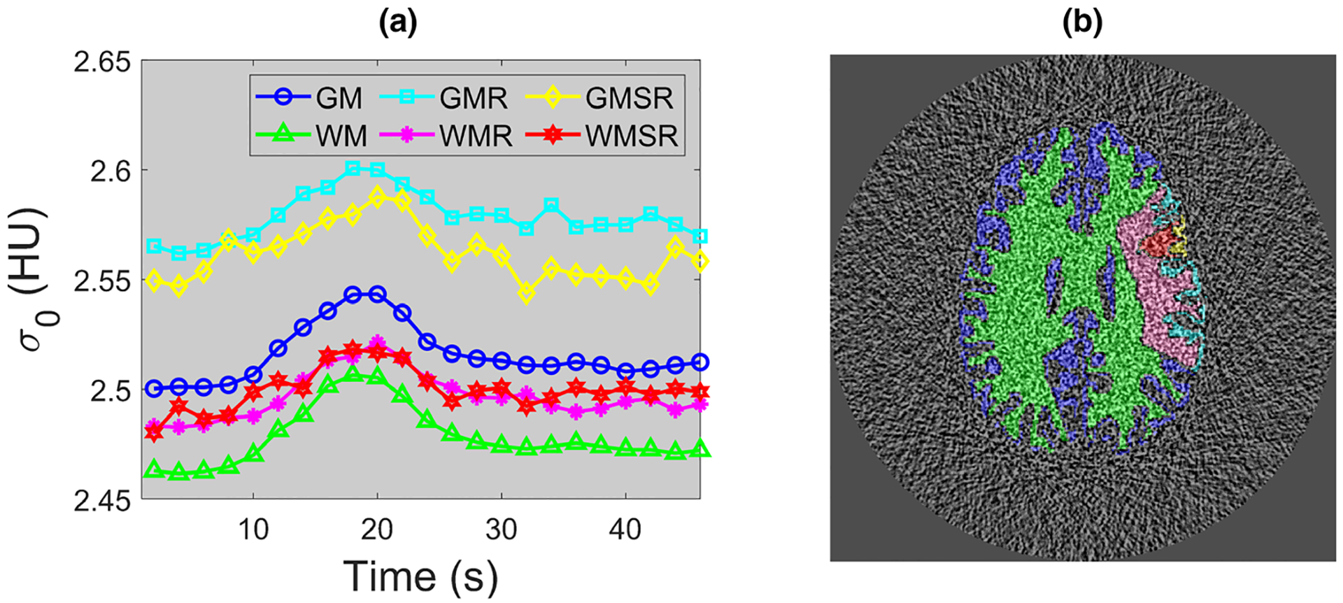
Numerical phantom results: (a) source image noise standard deviation (σ₀) measured at 100% dose level for each time frame and tissue type. Notice the narrow display range for the vertical axis. 95% of the σ₀ values lie within [97%,103%] × 2.52 HU. (b) An example noise-only source image. The color overlay illustrates pixels locations of each brain tissue type where σ₀ was measured. The legend in (a) also applies to (b).

Figure 4 plots measured and theoretical σ_CBV as a function of σ₀. The theoretical σ_CBV was calculated from σ₀ based on Eq. (12). Besides the agreement between measured and theoretical σ_CBV values, Fig. 4 also validates that σ_CBV is linearly proportional to σ₀. In addition, Fig. 4 demonstrates that the noise magnitude of CBV does not have any major dependence on tissue type or perfusion property. Unlike σ_CBV, the mean value of CBV did not demonstrate any dependence on radiation dose: as shown in Fig. 5, $\overline{\text{CBV}}$ remained quite stable across different dose levels, including the acquisition with the optimal dose partition. Example CBV images simulated at different radiation dose levels are provided in Fig. 6.

FIG. 4.

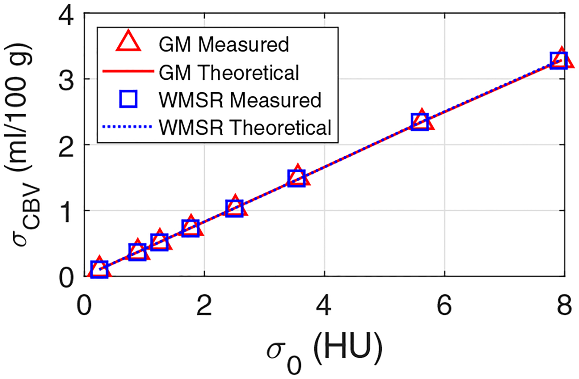
Numerical phantom results: theoretical and measured noise standard deviation of cerebral blood volume (CBV) (σ_CBV) plotted as a function of CT noise standard deviation (σ₀). GM: grey matter; WMSR: white matter with severely reduced blood flow.

FIG. 5.

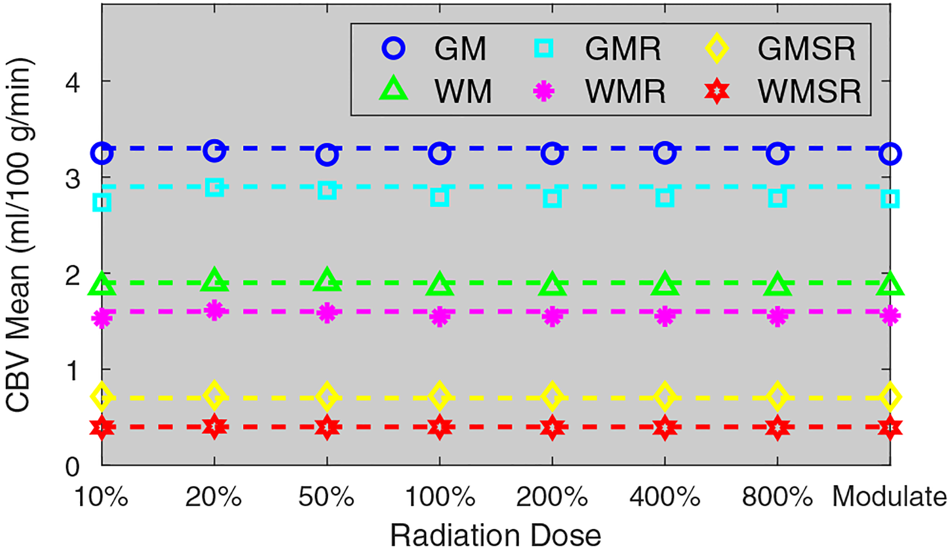
Numerical phantom results: mean cerebral blood volume (CBV) values of different brain tissues measured at different dose levels. The dashed lines are reference mean CBV values. The term “Modulate” denotes the computed tomography perfusion acquisition with the optimal dose partitioning at the 100% dose level.

FIG. 6.

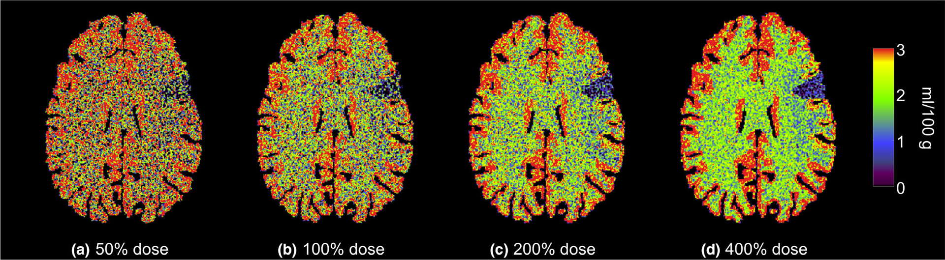
Numerical phantom results: cerebral blood volume maps generated at four different radiation dose levels. The color map also applied to Fig. 7.

Figure 7 compares CBV maps generated with the uniform dose partition method and the optimized dose partition method. The corresponding σ_CBV values are shown in Fig. 8. Compared with uniform dose partition, σ_CBV was reduced by 43% using the optimized dose partition method.

FIG. 7.

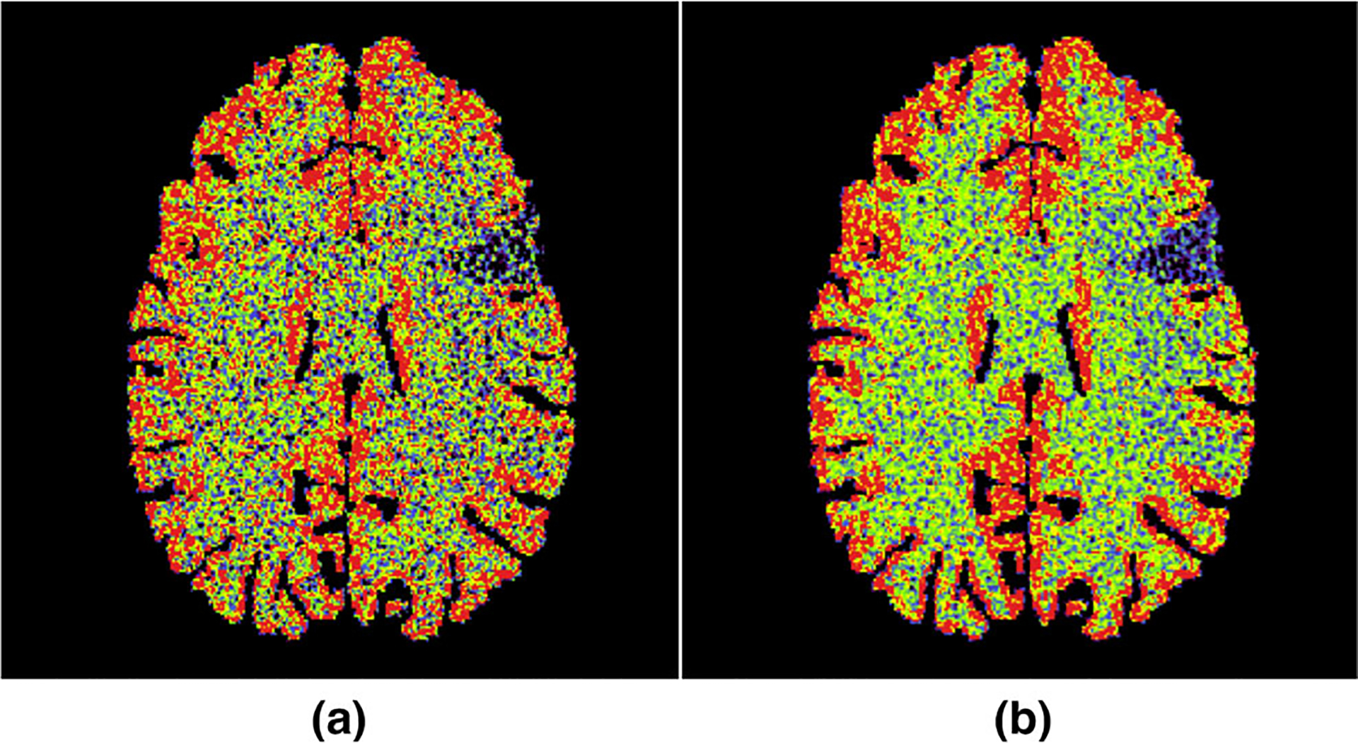
Numerical phantom results: (a) cerebral blood volume (CBV) map generated using uniform dose partition; (b) CBV map generated using the optimized dose partition. Both (a) and (b) were acquired at the 100% dose level.

FIG. 8.

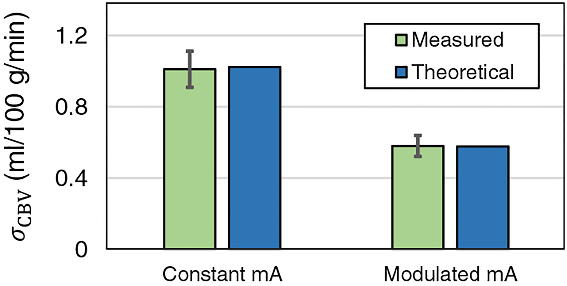
Numerical phantom results: comparison of σ_CBV of healthy grey matter for uniform (constant mA) and optimized (modulated mA) dose partitions. The theoretical values were calculated using Eq. (12) and σ₀.

4.B. Results of in vivo animal experiments

Figure 9 shows the measured and theoretical σ_CBV as a function of σ₀ for the three canine subjects. For both healthy and ischemic tissues, the theoretical values were consistent with the experimental results, and the linear relationship between σ_CBV and σ₀ was also confirmed.

FIG. 9.

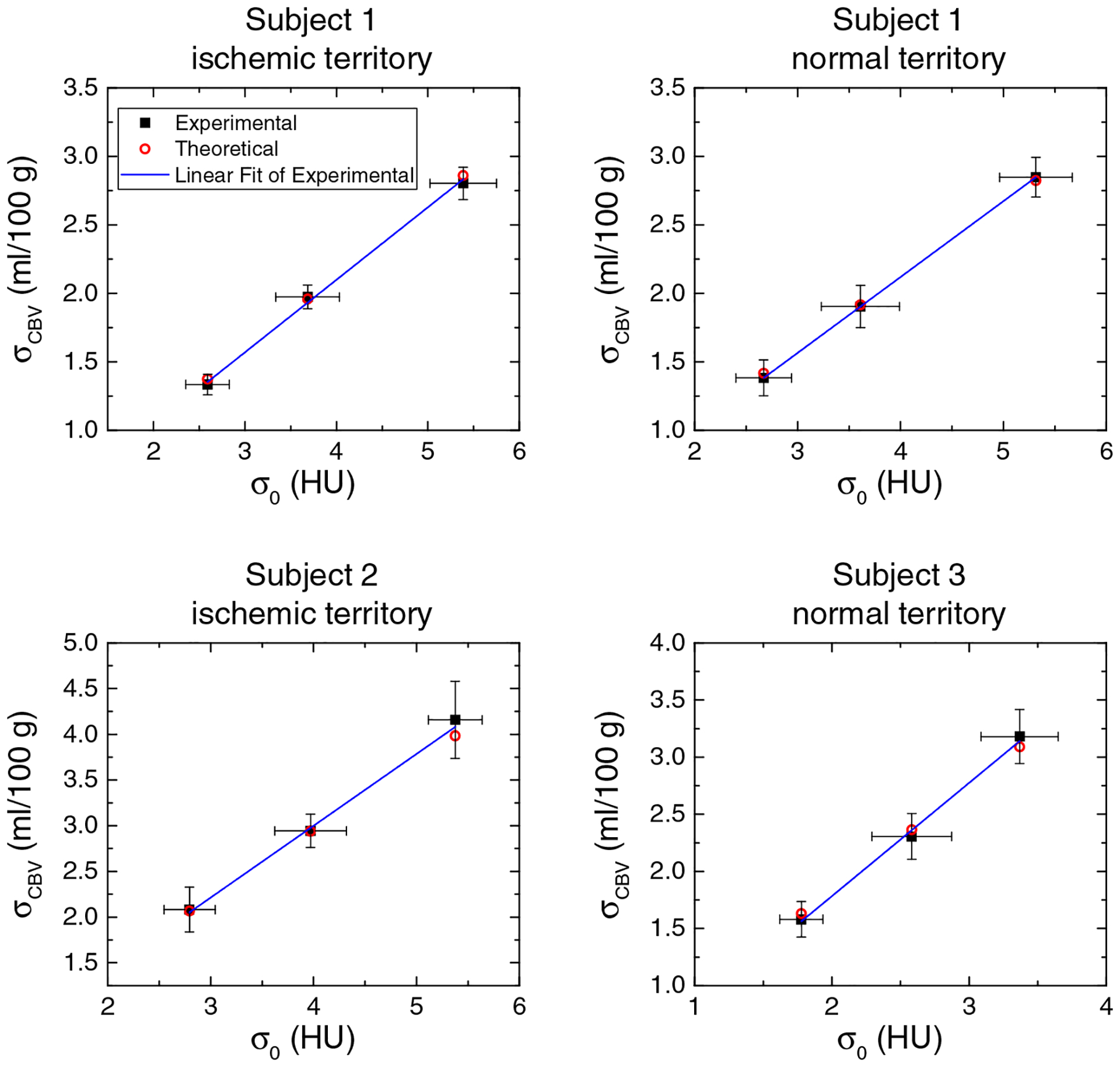
In vivo canine results: experimental and theoretical noise standard deviation of cerebral blood volume (CBV) (σ_CBV) plotted as a function of σ₀ for the three canine subjects. The error bars denote 95% confidence interval.

Figure 10 shows representative CBV maps of three canine subjects acquired at 98 mGy. Compared with uniform dose partition, the optimized dose partition method produced CBV maps with lower noise. For Subject 1 and Subject 2 that contain ischemic infarctions, the differentiation between normal tissues and ischemic territory (CBV < 1 ml/100 g) was effectively improved by the proposed dose partition method due to noise reduction. Meanwhile, the mean CBV values shown in Table II validated that the method did not introduce bias to CBV.

FIG. 10.

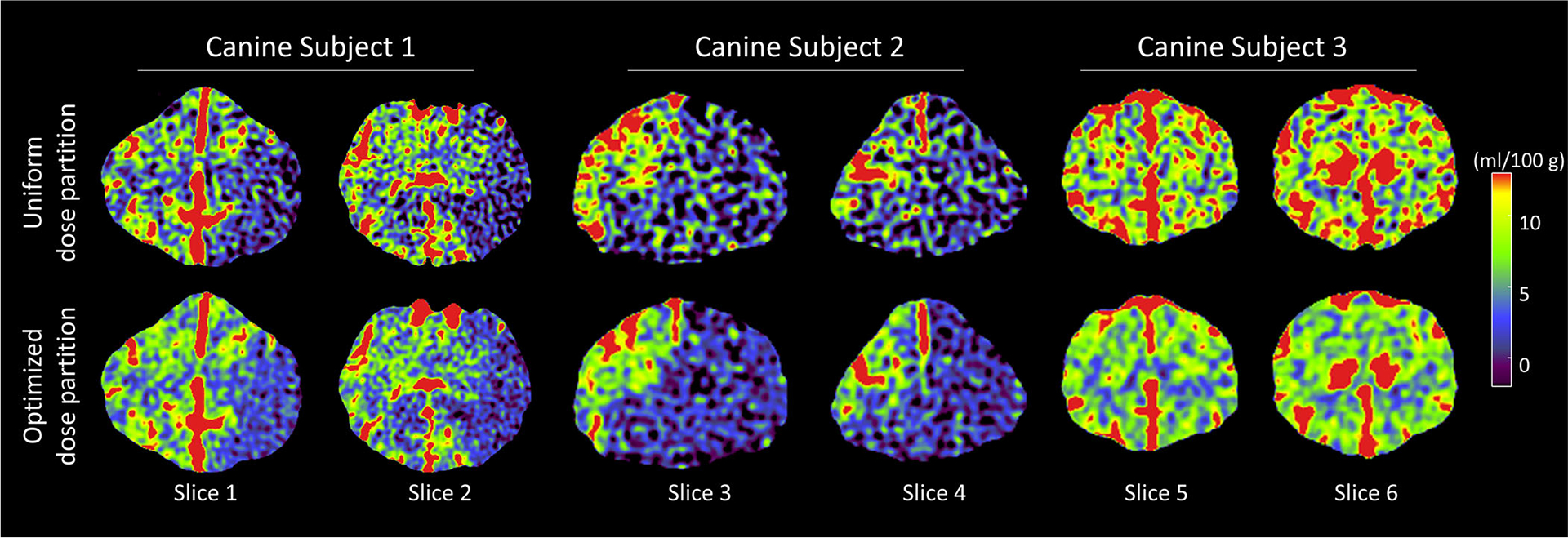
Cerebral blood volume images of the three in vivo canine subjects. Images in the top row and bottom row were acquired using conventional uniform dose partition and optimized dose partition, respectively. CTDI_vol of each computed tomography perfusion scan was 98 mGy.

Table II.

In vivo canine results: comparison of the measured mean $(\overline{\text{CBV}})$ and noise standard deviation (σ_CBV) of canine CBV maps acquired using the uniform and optimized dose partition methods.

	$\overline{\text{CBV}}$ (ml/100 g)		σCBV (ml/100 g)
Measurement location	Uniform	Optimized	Uniform	Optimized
Subject 1 normal territory	5.33	5.41	2.85	1.87
Subject 1 ischemic territory	0.55	0.57	2.80	1.92
Subject 2 ischemic territory	0.44	0.45	4.16	2.19
Subject 3 normal territory	5.01	4.94	3.18	1.57

5. DISCUSSION

Results of the digital phantom study and the animal experiments are consistent with the theory in Section 2, which states that the noise magnitude of CBV is linearly proportional to the noise magnitude of source images. Consequentially, CBV noise can be effectively reduced using reconstruction and postprocessing methods that suppress source image noise.^41,42,45,46

The theory also stated that the dependence of CBV noise on baseline and postbaseline images is different. An effective approach to reduce CBV noise is to repartition the total radiation dose: instead of uniformly distributing the dose over time, the total baseline dose should equal the combined dose delivered to other time frames. To reach this condition, dose per frame can be increased for the baseline frames if the number of baseline frames (N_b) is smaller than that of nonbaseline frames. If a CT system’s dose rate cannot be modulated during a CTP scan, an alternative implementation method is to increase N_b by using a longer baseline time window or shorter interframe interval (Δt).

Although this paper focused on the statistical properties of CT-derived CBV maps, the theoretical framework can be potentially extended to magnetic resonance (MR) perfusion imaging, which also uses Eq. (1) to derive the CBV map. Unlike the x-ray attenuation signal in CT, the MR signal is not linearly related to the concentration of the contrast agent (usually gadolinium), and the following formula can be used to convert the signal of MR source images S to contrast concentration C:^40,47

$$C(\overrightarrow{x},t)=-\frac{k_{\text{mr}}}{\text{TE}}\left[\text{ln}S(\overrightarrow{x},t)-\text{ln}{S}_b(\overrightarrow{x},t)\right],$$ (27)

where k_mr is a numerical scaling factor, TE is the echo time of the MR sequence. Based on Eqs. (1) and (27), a quantitative relationship between MR perfusion source image noise and CBV noise may be derived in a similar way as presented in this paper. However, it is important to point out that the radiation dose partition method developed for CTP is not applicable to MR perfusion imaging since it does not use ionizing radiation. In addition, modulating MR source image SNR over time may not be as straightforward as in CT.

This work has the following limitations. First, the study did not cover the noise covariance and spatial resolution of CBV maps, both of which are important aspects of CBV image quality. Second, the proposed dose partition strategy is optimized only for CBV and is not necessarily optimal for other parametric perfusion maps. Third, a clinical implementation of the optimal dose partition strategy may encounter several technical challenges such as limitations in the maximal tube current. Potential stochastic radiation effect associated with instantaneously higher x-ray exposure at baseline frames may also be a concern since the exact biological effect at the corresponding dose rate level is yet unknown. Fourth, it was assumed that CBV is calculated based on Eq. (1), although several other CBV calculation methods may also be used in practice. For example, one alternative method is to calculate the ratio between the peak of the tissue enhancement curve and the peak of the AIF in lieu of dividing the two full integrals (A and B). A different statistical model needs to be developed for this maximal value-based CBV estimation method. Another method to calculate CBV is to deconvolve tissue enhancement curve with the arterial enhancement curve to estimated the so-called flow-scaled residue function, whose temporal integration also leads to CBV.⁴⁰ For CBV generated from deconvolution-based CTP systems, its statistical properties are presented in the Part II paper.

6. CONCLUSIONS

Through a cascaded systems analysis of nondeconvolution-based CTP imaging systems, it was found that the noise of CBV maps is linearly related to the noise of CTP source images. In particular, CBV noise has a stronger dependence on the baseline image noise than nonbaseline noise, suggesting a CBV noise reduction opportunity via radiation dose modulation.

APPENDIX I

NOISE VARIANCE OF CBV

The analysis starts by deriving the noise variance formula for term A in Eq. (8). To save space, the $\overrightarrow{x}$ dependence in A is temporarily ignored. By definition, its noise variance is given by

$$\begin{gathered} {\sigma }_A^2=\overline{{(A-\overline{A})}^2} \\ =\stackrel{T}{\int }\underset{T_b}{\int }\left[\overline{\Delta I(t)\Delta I\left(t^{\prime }\right)}-\overline{\Delta I(t)\Delta I_b}-\overline{\Delta I\left(t^{\prime }\right)\Delta I_b}+\overline{{\Delta }^2{I}_b}\right]\text{d}t\text{d}{t}^{\prime } \\ =\stackrel{T}{\int }\underset{T_b}{\int }\overline{\Delta I(t)\Delta I\left(t^{\prime }\right)}\text{d}t\text{d}{t}^{\prime }-0-0+\overline{{\Delta }^2{I}_b}\stackrel{T}{\int }\underset{T_b}{\int }\text{d}t\text{d}{t}^{\prime } \\ =\stackrel{T}{\int }\underset{T_b}{\int }{\delta }_{t,t^{\prime }}\overline{\Delta I(t)\Delta I\left(t^{\prime }\right)}\text{d}t\text{d}{t}^{\prime }+{\sigma }_b^2{\left(T-T_b\right)}^2. \end{gathered}$$ (A1)

The use of the Kronecker delta function δ_t,t′ in Eq. (A1) is associated with the assumption that source image noise is uncorrelated along the temporal direction. Using the properties of Kronecker delta, δ_t,t′ = Δt δ(t – t′), Eq. (A2) can be further to Similarly, to

$$\begin{gathered} {\sigma }_A^2=\Delta t\stackrel{T}{\int }\underset{T_b}{\int }\delta \left(t-t^{\prime }\right)\overline{\Delta I(t)\Delta I\left(t^{\prime }\right)}\text{d}t\text{d}{t}^{\prime }+{\left(T-T_b\right)}^2{\sigma }_b^2 \\ =\Delta t{\int }_{T_b}^T\overline{{[\Delta I(t)]}^2}\text{d}t+{\left(T-T_b\right)}^2{\sigma }_b^2 \\ =\Delta t\left(T-T_b\right){\sigma }_0^2+{\left(T-T_b\right)}^2{\sigma }_b^2. \end{gathered}$$ (A2)

Similarly, it can be show that

$${\sigma }_B^2=\mathrm{\Delta }t\left(T-T_b\right){\sigma }_0^2+{\left(T-T_b\right)}^2{\sigma }_b^2.$$ (A3)

Based on the signal model of CBV in Eq. (8) and the general rule of error propagation, the noise variance of CBV is related to ${\sigma }_A^2$ and ${\sigma }_B^2$ by

$${\sigma }_{\text{CBV}}^2={\left(\frac{\partial \text{CBV}}{\partial A}\right)}_{\overline{A},\overline{B}}^2{\sigma }_A^2+{\left(\frac{\partial \text{CBV}}{\partial B}\right)}_{\overline{A},\overline{B}}^2{\sigma }_B^2+2{\left(\frac{\partial \text{CBV}}{\partial A}\frac{\partial \text{CBV}}{\partial B}\right)}_{\overline{A},\overline{B}}{\sigma }_{AB},$$ (A4)

where σ_AB denotes the covariance between A and B. Unless $\overrightarrow{x}$ and ${\overrightarrow{x}}_0$ are in close proximity, the covariance term σ_AB is usually negligible. Under this assumption, Eq. (A4) can be approximated by

$$\begin{gathered} {\sigma }_{\text{CBV}}^2\approx {\left(\frac{\partial \text{CBV}}{\partial A}\right)}_{\overline{A},\overline{B}}^2{\sigma }_A^2+{\left(\frac{\partial \text{CBV}}{\partial B}\right)}_{\overline{A},\overline{B}}^2{\sigma }_B^2 \\ ={\left(\frac{\kappa }{\overline{B}}\right)}^2{\sigma }_A^2+{\left(\frac{\kappa \overline{A}}{{\overline{B}}^2}\right)}^2{\sigma }_B^2 \\ ={\left(\frac{\kappa \overline{A}}{\overline{B}}\right)}^2\left[{\left(\frac{{\sigma }_A}{\overline{A}}\right)}^2+{\left(\frac{{\sigma }_B}{\overline{B}}\right)}^2\right]. \end{gathered}$$ (A5)

As shown by the human subject data in Figs. 11(a)–11(c) that were collected in an IRB-approved stroke imaging study, B (area under the baseline-corrected arterial enhancement curve) is usually an order of magnitude higher than A (area under the baseline-corrected tissue enhancement curve). In addition, Fig. 11(d) shows a noise-only CTP source image produced by subtracting two consecutive frames acquired at the peak of AIF. No significant variation of noise magnitude across vessel and parenchyma locations was observed. Therefore, σ_A and σ_A can be considered within the same order of magnitude, and thus the following assumption can be made:

$${\left(\frac{{\sigma }_A}{\overline{A}}\right)}^2\gg {\left(\frac{{\sigma }_B}{\overline{B}}\right)}^2.$$ (A6)

With this assumption, Eq. (A5) approximates the following form:

$$\begin{gathered} {\sigma }_{\text{CBV}}^2\approx {\left(\frac{\kappa }{\overline{B}}\right)}^2{\sigma }_A^2 \\ ={\left(\frac{\kappa }{\overline{B}}\right)}^2\left[\Delta t\left(T-T_b\right){\sigma }_0^2+{\left(T-T_b\right)}^2{\sigma }_b^2\right] \\ ={\left(\frac{\kappa \Delta t}{\overline{B}}\right)}^2\left[\left(N-N_b\right){\sigma }_0^2+{\left(N-N_b\right)}^2{\sigma }_b^2\right], \end{gathered}$$ (A7)

where (N – N_b) = (T − T_b)/Δt is the number of nonbaseline frames.

FIG. 11.

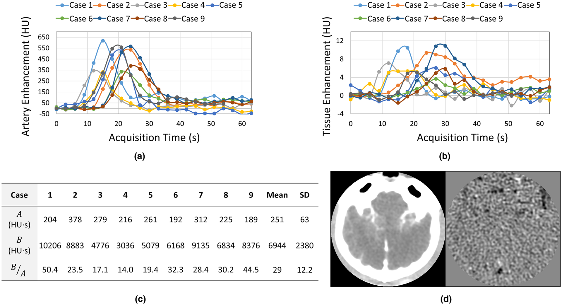
(a) Arterial enhancement curves measured in nine human subjects enrolled in an IRB-approved study. (b) Tissue enhancement curves of the same group of subjects. (c) Comparison of A (area under the tissue enhancement curve) and B (area under the tissue enhancement curve) for the same group of subjects. SD: standard deviation. (d) A peak enhancement source image frame and the corresponding noise-only image of a canine subject.

APPENDIX II

OPTIMAL DOSE PARTITION

The constrained multivariate optimization problem in Eqs. (17) and (18) is equivalent to the following unconstrained single variate optimization problem:

$$D_b^{*}=\underset{D_b}{\text{arg}\text{min}}\left[\frac{1}{D-N_b{D}_b}+\frac{1}{N_b{D}_b}\right].$$ (A8)

$D_b^{*}$ can be solved by

$$\begin{gathered} 0={\frac{\partial \left[{\left(D-N_b{D}_b\right)}^{-1}+{\left(N_b{D}_b\right)}^{-1}\right]}{\partial D_b}|}_{D_b=D_b^{*}} \\ =N_b\left[{\left(D-N_b{D}_b^{*}\right)}^{-2}-{\left(N_b{D}_b^{*}\right)}^{-2}\right]. \end{gathered}$$ (A9)

Solution of Eq. (A9) is

$$D_b^{*}=\frac{D}{2N_b}.$$ (A10)

Based on Eqs. (18) and (A10), $D_a^{*}$ is given by

$$D_a^{*}=\frac{D-N_b{D}_b^{*}}{N_a}=\frac{D}{2N_a}.$$ (A11)

REFERENCES

- 1.Axel L Cerebral blood flow determination by rapid-sequence computed tomography: theoretical analysis. Radiology. 1980;137:679–686. [DOI] [PubMed] [Google Scholar]
- 2.Miles K, Hayball M, Dixon A, Miles K, Hayball M, Dixon A. Colour perfusion imaging: a new application of computed tomography. Lancet. 1991;337:643–645. [DOI] [PubMed] [Google Scholar]
- 3.Muir KW, Santosh C. Imaging of acute stroke and transient ischaemic attack. J Neurol Neurosurg Psychiatry. 2005;76:iii19–iii28. [DOI] [PMC free article] [PubMed] [Google Scholar]
- 4.Lev M Acute stroke imaging: what is sufficient for triage to endovascular therapies? Am J Neuroradiol 2012;33:790–792. [DOI] [PMC free article] [PubMed] [Google Scholar]
- 5.Rai T, Raghuram K, Carpenter JS, Domico J, Hobbs G. Pre-intervention cerebral blood volume predicts outcomes in patients undergoing endovascular therapy for acute ischemic stroke. J NeuroIntervent Surg. 2013;5:i25–i32. [DOI] [PubMed] [Google Scholar]
- 6.Jain A, Jain M, Kanthala A, et al. Association of CT perfusion parameters with hemorrhagic transformation in acute ischemic stroke. Am J Neuroradiol. 2013;34:1895–1900. [DOI] [PMC free article] [PubMed] [Google Scholar]
- 7.Tong E, Hou Q, Fiebach JB, Wintermark M. The role of imaging in acute ischemic stroke. Neurosurg Focus. 2014;36:E3. [DOI] [PubMed] [Google Scholar]
- 8.Campbell C, Mitchell PJ, Kleinig TJ, et al. Endovascular therapy for ischemic stroke with perfusion-imaging selection. N Engl J Med. 2015;372:1009–1018. [DOI] [PubMed] [Google Scholar]
- 9.Prabhakaran S, Patel S, Samuels J, McClenathan B, Mohammad Y, Lee V. Perfusion computed tomography in transient ischemic attack. Arch Neurol. 2011;68:85–89. [DOI] [PubMed] [Google Scholar]
- 10.Siket MS, Edlow J. Transient ischemic attack: an evidence-based update. Emerg Med Pract. 2013;15:1–26. [PubMed] [Google Scholar]
- 11.Mehta K, Mustafa G, McMurtray A, et al. Whole brain CT perfusion deficits using 320-detector-row CT scanner in TIA patients are associated with ABCD2 score. Int J Neurosci. 2014;124:56–60. [DOI] [PubMed] [Google Scholar]
- 12.Souillard-Scemama R, Tisserand M, Calvet D, et al. An update on brain imaging in transient ischemic attack. J Neuroradiol. 2015;42:3–11. [DOI] [PubMed] [Google Scholar]
- 13.Gelfand JM, Wintermark M, Josephson SA. Cerebral perfusion-CT patterns following seizure. Eur J Neurol. 2010;17:594–601. [DOI] [PubMed] [Google Scholar]
- 14.Sanelli P, Ugorec I, Johnson C, et al. Using quantitative CT perfusion for evaluation of delayed cerebral ischemia following aneurysmal subarachnoid hemorrhage. Am J Neuroradiol. 2011;32:2047–2053. [DOI] [PMC free article] [PubMed] [Google Scholar]
- 15.Killeen R, Gupta A, Delaney H, et al. Appropriate use of CT perfusion following aneurysmal subarachnoid hemorrhage: a bayesian analysis approach. Am J Neuroradiol 2014;35:459–465. [DOI] [PMC free article] [PubMed] [Google Scholar]
- 16.Mir A, Gupta A, Dunning L, et al. CT perfusion for detection of delayed cerebral ischemia in aneurysmal subarachnoid hemorrhage: a systematic review and meta-analysis. Am J Neuroradiol. 2014;35:866–871. [DOI] [PMC free article] [PubMed] [Google Scholar]
- 17.Dai W, Zhao Y, Zhang Z, et al. Role of CT perfusion imaging in evaluating the effects of multiple burr hole surgery on adult ischemic moyamoya disease. Neuroradiology. 2013;55:1431–1438. [DOI] [PMC free article] [PubMed] [Google Scholar]
- 18.Zhang J, Wang J, Geng D, Li Y, Song D, Gu Y. Wholebrain CT perfusion and CT angiography assessment of moyamoya disease before and after surgical revascularization: preliminary study with 256-slice CT. PLoS ONE. 2013;8:e57595. [DOI] [PMC free article] [PubMed] [Google Scholar]
- 19.Wintermark M, Sincic R, Sridhar D, Chien J. Cerebral perfusion CT: technique and clinical applications. J Neuroradiol. 2008;35:253–260. [DOI] [PubMed] [Google Scholar]
- 20.Berkhemer OA, Fransen PS, Beumer D, et al. A randomized trial of intraarterial treatment for acute ischemic stroke. N Engl J Med. 2015;372:11–20. [DOI] [PubMed] [Google Scholar]
- 21.Saver JL, Goyal M, Bonafe A, et al. Stent-retriever thrombectomy after intravenous t-PA vs t-PA alone in stroke. N Engl J Med. 2015;372:2285–2295. [DOI] [PubMed] [Google Scholar]
- 22.Goyal M, Demchuk AM, Menon BK, et al. Randomized assessment of rapid endovascular treatment of ischemic stroke. N Engl J Med. 2015;372:1019–1030. [DOI] [PubMed] [Google Scholar]
- 23.Zhu T, Jovin A, Aghaebrahim P, Michel WZ, Wintermark M. Does perfusion imaging add value compared with plain parenchymal and vascular imaging? J NeuroIntervent Surg. 2012;4:246–250. [DOI] [PubMed] [Google Scholar]
- 24.Gonzalez RG. Low signal, high noise and large uncertainty make CT perfusion unsuitable for acute ischemic stroke patient selection for endovascular therapy. J NeuroIntervent Surg. 2012;4:242–245. [DOI] [PubMed] [Google Scholar]
- 25.González RG, Copen WA, Schaefer PW, et al. The massachusetts general hospital acute stroke imaging algorithm: an experience and evidence based approach. J NeuroIntervent Surg. 2013;5:i7–i12. [DOI] [PMC free article] [PubMed] [Google Scholar]
- 26.Goyal M, Menon BK, Derdeyn CP. Perfusion imaging in acute ischemic stroke: let us improve the science before changing clinical practice. Radiology. 2013;266:16–21. [DOI] [PubMed] [Google Scholar]
- 27.Lev MH. Perfusion imaging of acute stroke: its role in current and future clinical practice. Radiology. 2013;266:22–27. [DOI] [PubMed] [Google Scholar]
- 28.Sanelli PC, Lev MH, Eastwood JD, Gonzalez RG, Lee TY. The effect of varying user-selected input parameters on quantitative values in CT perfusion maps. Acad Radiol. 2004;11:1085–1092. [DOI] [PubMed] [Google Scholar]
- 29.Thijs VN, Somford DM, Bammer R, Robberecht W, Moseley ME, Albers GW. Influence of arterial input function on hypoperfusion volumes measured with perfusion-weighted imaging. Stroke. 2004;35:94–98. [DOI] [PubMed] [Google Scholar]
- 30.Soares B, Dankbaar J, Bredno J, et al. Automated versus manual postprocessing of perfusion-CT data in patients with acute cerebral ischemia: influence on interobserver variability. Neuroradiology. 2009;51:445–451. [DOI] [PMC free article] [PubMed] [Google Scholar]
- 31.Kudo K, Sasaki M, Yamada K, et al. Differences in CT perfusion maps generated by different commercial software: quantitative analysis by using identical source data of acute stroke patients. Radiology. 2010;254:200–209. [DOI] [PubMed] [Google Scholar]
- 32.Ferreira RM, Lev MH, Goldmakher GV, et al. Arterial input function placement for accurate CT perfusion map construction in acute stroke. Am J Roentgenol. 2010;194:1330–1336. [DOI] [PMC free article] [PubMed] [Google Scholar]
- 33.Galinovic I, Brunecker P, Ostwaldt AC, Soemmer C, Hotter B, Fiebach JB. Fully automated postprocessing carries a risk of substantial overestimation of perfusion deficits in acute stroke magnetic resonance imaging. Cerebrovasc Dis. 2011;31:408–413. [DOI] [PubMed] [Google Scholar]
- 34.Murase K, Nanjo T, Ii S, et al. Effect of x-ray tube current on the accuracy of cerebral perfusion parameters obtained by CT perfusion studies. Phys Med Biol. 2005;50:5019. [DOI] [PubMed] [Google Scholar]
- 35.Cohnen M, Wittsack H-J, Assadi S, et al. Radiation exposure of patients in comprehensive computed tomography of the head in acute stroke. Am J Neuroradiol. 2006;27:1741–1745. [PMC free article] [PubMed] [Google Scholar]
- 36.Yamauchi-Kawara C, Fujii K, Aoyama T, Yamauchi M, Koyama S. Radiation dose evaluation in multidetector-row CT imaging for acute stroke with an anthropomorphic phantom. Br J Radiol. 2010;83:1029–1041. [DOI] [PMC free article] [PubMed] [Google Scholar]
- 37.Wintermark M, Lev M. FDA investigates the safety of brain perfusion CT. Am J Neuroradiol. 2010;31:2–3. [DOI] [PMC free article] [PubMed] [Google Scholar]
- 38.Li K, Chen G-H. Noise characteristics of CT perfusion imaging: how does noise propagate from source images to final perfusion maps?. Proc SPIE Medical Imaging 2016: Physics of Medical Imaging. 2016;9783:978310. [DOI] [PMC free article] [PubMed] [Google Scholar]
- 39.Konstas A, Goldmakher G, Lee T-Y, Lev M. Theoretic basis and technical implementations of CT perfusion in acute ischemic stroke part 1: theoretic basis. Am J Neuroradiol. 2009;30:662–668. [DOI] [PMC free article] [PubMed] [Google Scholar]
- 40.Fieselmann A, Kowarschik M, Ganguly A, Hornegger J, Fahrig R. Deconvolution-based CT and MR brain perfusion measurement: theoretical model revisited and practical implementation details. Int J Biomed Imaging. 2011;2011:20. [DOI] [PMC free article] [PubMed] [Google Scholar]
- 41.Manhart M, Kowarschik M, Fieselmann A, et al. Dynamic iterative reconstruction for interventional 4-D C-arm CT perfusion imaging. IEEE Trans Med Imag. 2013;32:1336–1348. [DOI] [PubMed] [Google Scholar]
- 42.Manhart MT, Aichert A, Struffert T, et al. Denoising and artefact reduction in dynamic flat detector CT perfusion imaging using high speed acquisition: first experimental and clinical results. Phys Med Biol. 2014;59:4505. [DOI] [PubMed] [Google Scholar]
- 43.Ahmed M, Zellerhoff C, Strother K, et al. C-arm CT measurement of cerebral blood volume: an experimental study in canines. Am J Neuroradiol. 2009;30:917–922. [DOI] [PMC free article] [PubMed] [Google Scholar]
- 44.Royalty K, Manhart M, Pulfer K, et al. C-arm CT measurement of cerebral blood volume and cerebral blood flow using a novel high-speed acquisition and a single intravenous contrast injection. Am J Neuroradiol. 2013;34:2131–2138. [DOI] [PMC free article] [PubMed] [Google Scholar]
- 45.Ma J, Zhang H, Gao Y, et al. Iterative image reconstruction for cerebral perfusion CT using a pre-contrast scan induced edge-preserving prior. Phys Med Biol. 2012;57:7519. [DOI] [PMC free article] [PubMed] [Google Scholar]
- 46.Niesten J, van der Schaaf I, Riordan A, et al. Radiation dose reduction in cerebral CT perfusion imaging using iterative reconstruction. Eur Radiol. 2014;24:484–493. [DOI] [PubMed] [Google Scholar]
- 47.Waldman D, Barker PB, Gillard JH, eds. Clinical MR Neuroimaging: Physiological and Functional Techniques, 2nd edn Cambridge, UK: Cambridge University Press; 2009. [Google Scholar]