Staining and Quantification of β-Amyloid Pathology in Transgenic Mouse Models of Alzheimer’s Disease

Abstract

Studies of Alzheimer’s disease (AD) using experimental systems most often involve transgenic mouse models that are characterized by neural accumulation of β-amyloid protein (Aβ), which is widely hypothesized to have a key role in AD pathogenesis. Quantification of Aβ in transgenic mice typically is accomplished through both biochemical and histochemical approaches. In this chapter, we describe two techniques for the histological detection of Aβ, immunostaining with Aβ antibodies and staining with the amyloid dye thioflavin S, and its quantification using digital imaging.

1. Introduction

AD neuropathology is characterized by multiple components but is typically defined by two primary lesions. The first is termed neurofibrillary tangles and are composed of insoluble, hyperphosphorylated forms of the microtubule associated protein tau [1]. The second is plaques, which are extracellular deposits of aggregated Aβ protein [1]. There is compelling evidence that both lesions prominently contribute to the initiation and/or progression of the disease [2], although Aβ has long been hypothesized to have the key pathogenic role [3] and has been the primary target for therapeutic intervention strategies [4]. Consequently, quantitative assessments of Aβ will continue to be important outcome measures for preclinical studies in transgenic mouse models of AD.

There are two widely used approaches for measurement of Aβ. First, brain levels of Aβ are effectively measured by ELISA following a sequential series of fractionation steps, as previously described [5]. This technique has the advantage of determining Aβ amounts in different states of peptide solubility but is limited spatially in terms of brain region specificity. The second approach is histological assessment. Extracellular and, in some cases, intracellular accumulations of aggregated Aβ deposits are detected by immunochemistry using antibodies directed against Aβ. In addition, fibrils of Aβ that have acquired β-sheet conformation characteristic of amyloids can be detected by several amyloid dyes, including thioflavin S. These two staining approaches yield subtle but important differences in that all Aβ deposits will be detected with Aβ immunochemistry, and a subset of these with thioflavin S. Histological approaches have the strength of precise regional quantification of Aβ burden but the disadvantage of assessing only larger accumulations of aggregated Aβ (i.e., not detecting various soluble forms of Aβ). We describe histological protocols for the detection and quantification of Aβ from mouse brain, including tissue preparation, Aβ immunochemistry with antigen unmasking, thioflavin S staining, and digital image acquisition and analysis of stained tissue.

2. Materials

1. Phosphate-buffered saline (PBS), pH 7.4 (137 mM NaCl, 10 mM phosphate, 2.7 mM KCl).

2. Sorenson’s phosphate buffer, pH 7.0–7.5 (80.4 ml 133 mM Na₂HPO₄; 19.6 ml 133 mM KH₂PO₄).

3. PBS with 0.03% sodium azide, pH 7.4.

4. Tris-buffered saline (TBS), pH 7.4 (0.137 M sodium chloride, 0.0027 M potassium chloride, and 0.025 M Tris/Tris-HCl).

5. 95% formic acid.

6. Quench buffer: TBS with 10% methanol, 3% H₂O₂ (freshly prepared).

7. TBS with 0.1% Triton-X (TBS-TX).

8. Blocking buffer: TBS with 2% bovine serum albumin.

9. Primary antibody: rabbit anti-amyloid β (Thermo Fisher, Cat #71–5800) diluted 1:300 in blocking buffer.

10. Secondary antibody: biotinylated goat anti-rabbit antibody (Vector Laboratories, Cat #BA-1000) diluted 1:1000 in blocking buffer.

11. Avidin-biotin solution: prepare 30 min prior to use using ABC reagents from VECTASTAIN Elite Standard ABC kit (Vector Laboratories, Cat #PK-6100) diluted into TBS.

12. 3´3´ Diaminobenzidine (DAB) solution: prepare fresh using Vector DAB kit.

13. Ethanol solutions: 50%, 70%, 95%, 100%.

14. Xylene.

15. Permanent mounting solution (e.g., Krystalon, Millipore, Cat #64969).

16. 1% thioflavin-S (Sigma, Cat #T-1892).

17. Anti-fade mounting medium (e.g., VECTASHIELD™ Hardset, Vector Laboratories, Cat #H-1400; or ProLong™ Gold, Thermo Fisher, Cat #P36930).

18. ImageJ software (imagej.nih.gov/ij/).

19. Sorenson’s phosphate buffer with 4% paraformaldehyde, pH 7.0–7.5.

3. Methods

3.1. Tissue Preparation

1. Collect mouse brains after perfusion with ice-cold PBS alone or PBS followed by perfusion with 4% paraformaldehyde in Sorenson’s phosphate buffer (see Note 1). If perfused with only PBS, brains are immediately placed into 4% paraformaldehyde and immersion fixed at 4 °C for 48–72 h. Store fixed brains at 4 °C in PBS/0.03% sodium azide until sectioning.

2. Section brains exhaustively in the horizontal plane at a thickness of 30–40 μm on a vibratome. Tissue should be collected and stored in a manner that maintains spatial ordering. This is readily accomplished by collecting sections singly into sterile 48-well plates, which can be sealed with Parafilm™ and stored at 4 °C in PBS/0.03% sodium azide; staining should be completed in a timely manner. Every eighth section containing the hippocampus is used for Aβ or thioflavin staining (see Note 2). The remaining sections can be used for other stains, as needed.

3.2. Amyloid β Immunohistochemistry

All procedures can be performed at room temperature, unless otherwise stated. All solutions should be thoroughly mixed prior to use. Sections should be placed on an orbital shaker during incubation and rinse periods.

1. Transfer brain sections into wells from a 24-well plate containing TBS (see Note 3). Each well should contain 1–5 sections. Use every eighth section per brain (8–10 sections per brain) (see Note 4).

2. Incubate sections in 95% formic acid for 5 min (see Note 5).

3. Rinse sections 3 × in TBS for 5 min.

4. Incubate sections for 10 min in quench buffer (see Note 6).

5. Rinse sections 3 × for 5 min in TBS-TX.

6. Incubate sections for 30 min in blocking buffer (see Note 7).

7. Incubate sections overnight in the primary antibody (see Note 8). This step should be performed at 4 °C and, if possible, on an orbital shaker set to low speed (see Note 9).

8. Rinse sections 3 × for 5 min in TBS-TX.

9. Incubate sections for 15 min in blocking buffer.

10. Incubate sections for 60 min in secondary antibody.

11. Rinse sections 3 × for 5 min in TBS-TX.

12. Incubate sections for 15 min in blocking buffer.

13. Incubate sections for 60 min in avidin-biotin solution.

14. Rinse sections 3 × for 5 min in TBS.

15. Transfer sections into the staining solution of 3^´3’ diaminobenzidine (DAB) (see Note 10) and incubate 5 min (see Note 11).

16. Rinse sections 3 × for 5 min in TBS.

17. Mount stained sections on glass microscope slides (see Note 12).

18. Dry slides with mounted sections overnight at room temperature or on a slide warmer.

19. Dehydrate air-dried sections by rinsing in a series of increasing alcohol solutions (see Note 13). All times are minimums.

    1. 1 × in 70% alcohol for 3 min.
    2. 1 × in 95% alcohol for 3 min.
    3. 2 × in 100% alcohol for 3 min.
    4. Dip in xylene.
    5. 1 × in xylene for 15 min (see Note 14).

20. Coverslip the slides one at a time (leaving remaining slides in xylene rinse) using a permanent mounting solution and allow to cure overnight (see Note 15).

3.3. Thioflavin-S Staining

1. Mount tissue sections on subbed glass slides and air dry overnight at room temperature.

2. Wash dried slides 3 × for 3 min each in 50% alcohol.

3. Dip slides in water then wash in purified water 1 × for 3 min.

4. Incubate slides for 10 min in 1% thioflavin S solution (see Note 16).

5. Wash slides 5 × times for 3 min each in 70% alcohol.

6. Wash slides 3 × for 3 min each in 50% alcohol (see Note 17).

7. Wash slides 2 × for 15 min each in purified water.

8. Air dry slides for 15–30 min.

9. Coverslip slides using an antifade mounting medium and store in darkness.

3.4. Imaging and Quantification of Amyloid β Immunohistochemical Load

1. Confirm optimized settings on light microscope with attached digital camera imaging system (see Note 18).

2. Place stained slide on microscope stage and locate hippocampal formation on amyloid β immunostained section. Capture non-overlapping digital images using the 20 × objective (see Note 19) (Fig. 1).

3. For image analysis, begin by opening Image J (NIH) software. Next, under the Analyze tab, choose Set Measurements and confirm that the Area, Area Fraction, and Limit to Threshold options are selected.

4. Open saved files and define the region of interest (ROI) by outlining with the polygon function located on the toolbar (see Note 20).

5. Convert images with defined ROI into 8-bit grayscale by selecting the following tabs in Image J: Image > Type > 8-bit.

6. Prior to quantification, grayscale images need to be converted to binary images in which each pixel is either black or white (Fig. 2). To perform this threshold function, select the tabs: Image > Adjust > Threshold. Select the predetermined threshold value (see Note 21).

7. To quantify the amount of positive immunolabeling (i.e., black pixels) within the ROI, select Analyze > Measure and record both “Area” (represents the total number of stained pixels within the ROI) and “Percent area” (represents the proportion of the ROI with positive labeling). For example, if you collect two images of subiculum, there will be Area1 and Area2 as well as Percent area1 and Percent area2 corresponding to the values for each image.

8. Calculate the ROI area, which will be the total number of pixels within the outlined area, for each image as: (100/percent area) * area. For example, from subiculum image 1 this will be calculated as follows:

   $$\left(100/\text{Percent area}1\right)*\text{Area}1=\text{Total area}1$$
9. Calculate the percent staining for the combined ROI of the subregion of the hippocampus for each section by adding the stained areas (given by Image J) divided by the sum of the total areas (calculated by the experimenter). This allows the experimenter to account for differences in sizes of ROIs. For example, the total percent staining in the subiculum will be calculated as:

   $$\left(\text{Area}1+\text{Area}2\right)/\left(\text{Total area}1+\text{Total area}2\right)*100=\text{amyloid }\mathrm{\beta }\text{ load of the subiculum of section }1$$

10. When all images for a specific animal have been quantified, average the total percent staining across all sections, yielding the amyloid β load (also referred to as immunohistochemical burden) for the subiculum and CA1 regions of the hippocampus. These values are suitable for statistical analyses.

Fig. 1.

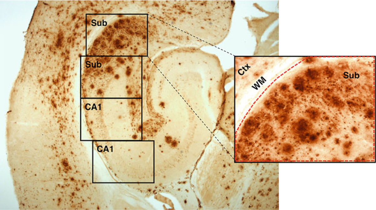
Illustration of image collection and region of interest determination. Horizontal section of EFAD transgenic mouse showing extensive pathology by amyloid β immunoreactivity using protocol described in Subheading 3.1. Boxes show pattern of image collection using 20 × objective for subiculum (Sub) and CA1 hippocampus (CA1). Inset shows larger view of first subiculum image. Using the polygon function, the region of interest (ROI) is defined (dotted red line) to include subiculum but not adjacent cortex (Ctx) and white matter (WM) (as described in Subheading 3.4)

Fig. 2.

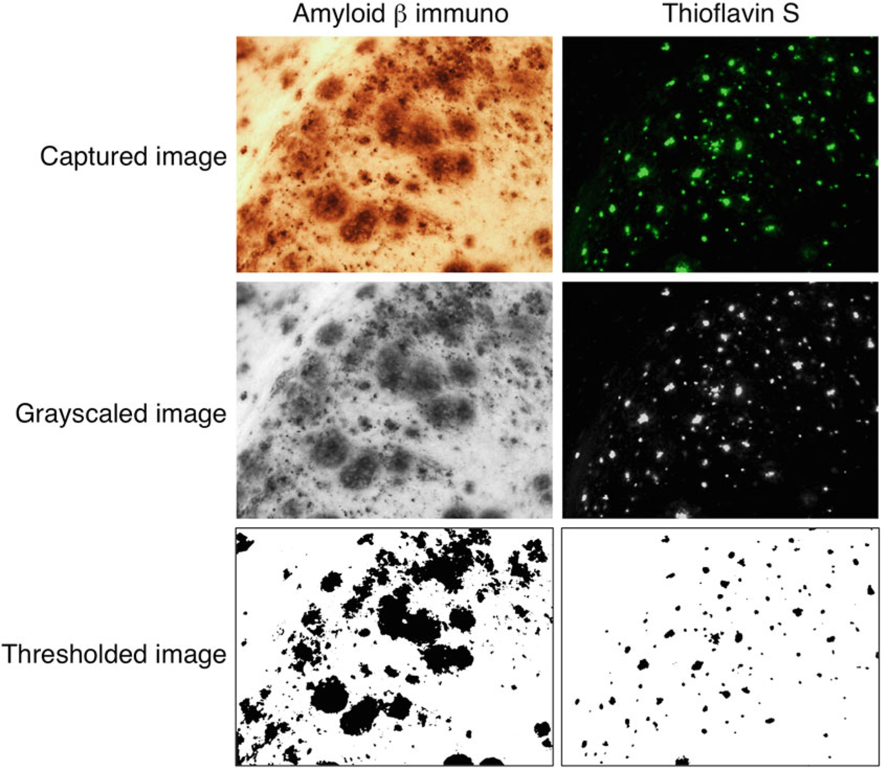
Examples of image transformation prior to quantification. Panels show a single microscopic field from subiculum in an EFAD transgenic mouse of either amyloid β immunoreactivity (left column) or thioflavin S staining (right column) at initial image collection of labeling (Captured image), following conversion to grayscale (Grayscaled image), and after the threshold step (Thresholded image). The thresholded images are suitable for quantification (described in Subheadings 3.4 and 3.5). Note that the ROI is not shown

3.5. Imaging and Quantification of Thioflavin Staining

1. Visualize thioflavin-stained sections using an epifluorescence microscope with a 20 × objective (see Note 22).

2. Capture images of the hippocampus as described for amyloid β immunoreactivity (Subheading 3.5, step 2) and save as TIFF files.

3. Calibrate Image J to measure plaque size in μm rather than pixels (see Note 23).

4. Next, under the Analyze tab, select Set Measurements and make sure Area and Limit to Threshold are selected.

5. Open images of thioflavin-stained sections in Image J and convert to 8-bit grayscale images by selecting the following tabs: Image > Type > 8-bit.

6. Convert grayscale to binary images by selecting the tabs: Image > Adjust > Threshold using a predetermined threshold value (see Note 24).

7. In the Threshold menu, select the box that says “Dark background.” This will invert the image so that the plaques will appear black against a white background.

8. To quantify plaque size, use the Ellipse tool to place circles around individual plaques. Under the Analyze tab, select Measure (see Note 25).

9. Record all plaque sizes (listed as area in μm²) in a separate file (e.g., Excel) (see Note 26).

4. Notes

1. Tissue can also be collected and stored using cryopreservation techniques.

2. Sectioning in the horizontal plane allows excellent visualization of hippocampal subfields across the hippocampus. Approximately 90 sections of 40 μm that contain hippocampus are generated by exhaustive sectioning of mouse brain. Sectioning in other planes and/or at other tissue thicknesses may require modifications in microscope settings, and image collection and processing (Subheading 3.4).

3. A fine paintbrush is used to gently move the sections from well to well. However, several other methods of tissue movement or solution change can be used, including glass probes, net wells, and light suction. It is recommended to transfer sections down to adjacent wells for each step, moving left to right across a 24-well plate oriented to yield four rows and six columns.

4. Ideally, immunostaining runs should be balanced across experimental groups to control for inter-experiment variability.

5. This is an antigen-unmasking step that is essential for robust Aβ immunostaining [6]. Formic acid is flammable and toxic. Appropriate PPE including lab coats, gloves, and eye protection should be worn, and formic acid should be manipulated in a chemical fume hood.

6. This solution must be prepared immediately prior to use due to the labile nature of hydrogen peroxide. This step serves to quench endogenous peroxidases that can interfere with visualization.

7. Solution should be freshly prepared. This step is used to block nonspecific labeling. Depending upon the primary antibody, the level of blocking component in the buffer may need to be increased up to 5% BSA, 1–5% normal serum, or a combination of BSA and serum.

8. In addition to the described primary antibody (Thermo Fisher, Cat #71–5800), other anti-amyloid β antibodies (e.g., MOAB2) can be substituted but the dilution will need to be optimized. The inclusion of 0.1% TX may be useful with some antibodies to minimize nonspecific binding.

9. If a refrigerated shaker is not available, sections can be stored without shaking in at 4 °C overnight. In this case, sections should remain on the room temperature shaker for a few hours before storage, if possible.

10. DAB is a suspected carcinogen and should be handled carefully including use of appropriate PPE and engineering controls. We use DAB kits from Vector Laboratories (Cat #SK-4100), preparing the solution immediately prior to use according to manufacturer’s instructions. This kit and others that use soluble DAB reduce the risk of contamination, but DAB solutions are still toxic. Disposal of DAB requires decontamination, which is best achieved by adding to an equal volume of a 1:1 0.2 M potassium permanganate and 2 M sulfuric acid solution. The final solution is then two parts DAB, one part potassium permanganate, and one part sulfuric acid. Although this solution is thought to completely decontaminate DAB, we collect it and dispose of it as a hazardous chemical.

11. Optimal incubation times in DAB solution are affected by various parameters (primary and secondary antibodies, temperature, rodent strain, etc.) but are usually between 4 and 8 min. Incubation time in DAB may need to be optimized and should remain constant within an experiment.

12. Slides should be either subbed (precoated with gelatin solution) or commercially prepared tissue slides (e.g., Superfrost® Plus slides), both of which facilitate tissue adhesion. Mounting sections in sequential order (4–10 per slide) is preferred and is easily accomplished by transferring sections onto a slide partially submerged in a small dish filled with TBS.

13. Alcohol solutions should be replaced regularly. We use histological grade reagent alcohol (Thermo Fisher, Cat #A962-P4).

14. All dehydration rinses should be performed in a chemical fume hood. Xylene is toxic and should be used with appropriate PPE including lab coat, nitrile gloves, and goggles.

15. We use Krystalon (Millipore, Cat #64969) as a mounting medium, but other similar media are suitable including Per-mount (Thermo Fisher, Cat #SP15) and DPX (Sigma, Cat #06522). All listed mounting media are toxic and flammable and should be used only in a chemical fume hood with appropriate PPE. After curing overnight, excess mounting media can be removed from coverslipped slides by scraping with a razor.

16. One percent thioflavin-S (Sigma, Cat #T-1892) should be made by adding thioflavin powder slowly to rapidly stirring purified water. When the powder is fully dissolved, filter the solution through #1 Whatman filter paper. Thioflavin solution should be made fresh but can be stored in foil-wrapped bottle in a dark cupboard for up to 2 weeks.

17. Steps 6–9 describe the process for storing stained sections in a fluorescent antifade solution. Another option is to dehydrate and coverslip without antifade. In this case, replace steps 6–9 with steps 19 and 20 described in Subheading 3.1.

18. The optical settings on the microscope (e.g., centering and intensity of light, condenser focus) should be optimized prior to image collection. The depth of field should be adjusted to a relatively collapsed setting such that most of the staining is in focus. We generally use a setting between 0.4 and 0.6, depending upon the transgenic mouse line. The exposure time should also be optimized. For our system, one-third overexposure generally yields images with the highest signal–noise relationship. Optimized settings should be held constant across all image collections for a given study.

19. Typically, we collect two images of subiculum and three of cornu Ammonis 1 (CA1) per section. Additional hippocampal subfields can be imaged similarly as can entorhinal cortex, which is located superior to hippocampal formation. It may be most practical to limit image collection to the sections with well-defined hippocampal subfields. We find it best to save images as TIFF files.

20. Images usually include areas in addition to the specific brain regions that should be excluded from the ROI. Subiculum images often contain cortex, a portion of CA1 and/or adjacent white matter. In some CA1 images, the hippocampal fissure will be visible. See Fig. 1 for an example.

21. Properly adjusting the threshold will maximize the amount of specific immunoreactivity and minimize nonspecific staining. The proper threshold setting can be affected by several variables including optical (e.g., depth of field), tissue-related (e.g., tissue thickness, transgenic strain), and immunochemistry quality. The optimal threshold setting must be empirically determined by comparing regions of specific and nonspecific immunostaining on grayscale images with corresponding regions on binary images. We find that within specific strains of Alzheimer’s transgenic mice, an optimal threshold setting can be applied to all animals. For example, with EFAD mice sectioned at 40 μm and stained as described under Subheading 3.2, we use a threshold setting of 95. There are instances in which, even within the same immunostaining run, different animals exhibit somewhat lower or higher levels of background immunoreactivity. In these cases, all sections from a lightly stained animal would be thresholded using a predetermined increment (e.g., 5–10 U) above the standard. Conversely, sections from a darkly stained animal would be thresholded at a slightly lower setting. Generally, such animals comprise <10% of all animals. The threshold value should be the same for all sections from each animal.

22. Thioflavin can be viewed using both blue (green light, used for FITC) and ultraviolet (blue light, used for DAPI) filters. The user will need to determine which has the best contrast for their use.

23. We calibrate using a stage micrometer, which is imaged using the same final magnification as the images to be analyzed. Open the image of the stage micrometer in Image J and select Calibration tab. Using the computer mouse, trace a defined length and enter the corresponding value (e.g., 100 μm). The program will now convert pixels to microns.

24. As with amyloid β immunoreactivity, the threshold value must be optimized. However, because thioflavin S staining typically shows low background in mouse brain and is not subject to the variability inherent to immunochemistry, determining the thioflavin threshold is straightforward and does not require correction.

25. You do not need to closely trace the plaque when using the Ellipse tool. The software will measure only the labeled pixels. However, make sure to include only one plaque in each ellipse.

26. In addition to quantifying plaque areas, you can simply sum the number of measured plaques to generate plaque number. These data can be further refined into plaque density by expressing as a function of area. In addition, the thioflavin load or burden can be determined as described for amyloid β immunoreactivity (Subheading 3.4) using thioflavin-labeled sections.

References

- 1.Vinters HV (2015) Emerging concepts in Alzheimer’s disease. Annu Rev Pathol 10:291–319 [DOI] [PubMed] [Google Scholar]
- 2.Bloom GS (2014) Amyloid-β and tau: the trigger and bullet in Alzheimer disease pathogenesis. JAMA Neurol 71:505–508 [DOI] [PubMed] [Google Scholar]
- 3.Selkoe DJ, Hardy J (2016) The amyloid hypothesis of Alzheimer’s disease at 25 years. EMBO Mol Med 8:595–608 [DOI] [PMC free article] [PubMed] [Google Scholar]
- 4.Sala Frigerio C, De Strooper B (2016) Alzheimer’s disease mechanisms and emerging roads to novel therapeutics. Annu Rev Neurosci 39:57–79 [DOI] [PubMed] [Google Scholar]
- 5.Schmidt SD, Mazzella MJ, Nixon RA, Mathews PM (2012) Aβ measurement by enzyme-linked immunosorbent assay. Methods Mol Biol 849:507–527 [DOI] [PubMed] [Google Scholar]
- 6.Cummings BJ, Mason AJL, Kim RC, Sheu PC-Y, Anderson AJ (2002) Optimization of techniques for the maximal detection and quantification of Alzheimer’s-related neuropathology with digital imaging. Neurobiol Aging 23:161–170 [DOI] [PubMed] [Google Scholar]