

Abstract
Dissecting the genetic mechanism underlying a complex disease hinges on discovering gene–environment interactions (GXE). However, detecting GXE is a challenging problem especially when the genetic variants under study are rare. Haplotype-based tests have several advantages over the so-called collapsing tests for detecting rare variants as highlighted in recent literature. Thus, it is of practical interest to compare haplotype-based tests for detecting GXE including the recent ones developed specifically for rare haplotypes. We compare the following methods: haplo.glm, hapassoc, HapReg, Bayesian hierarchical generalized linear model (BhGLM) and logistic Bayesian LASSO (LBL). We simulate data under different types of association scenarios and levels of gene–environment dependence. We find that when the type I error rates are controlled to be the same for all methods, LBL is the most powerful method for detecting GXE. We applied the methods to a lung cancer data set, in particular, in region 15q25.1 as it has been suggested in the literature that it interacts with smoking to affect the lung cancer susceptibility and that it is associated with smoking behavior. LBL and BhGLM were able to detect a rare haplotype–smoking interaction in this region. We also analyzed the sequence data from the Dallas Heart Study, a population-based multi-ethnic study. Specifically, we considered haplotype blocks in the gene ANGPTL4 for association with trait serum triglyceride and used ethnicity as a covariate. Only LBL found interactions of haplotypes with race (Hispanic). Thus, in general, LBL seems to be the best method for detecting GXE among the ones we studied here. Nonetheless, it requires the most computation time.
Keywords: gene–environment independence, regularization, lung cancer, triglycerides, Dallas Heart Study
Introduction
Detecting gene–environment interactions (GXE) is critical for unraveling the etiology of complex diseases [1]. At the same time, in the past decade, the search for rare variants has been at the forefront of the research efforts [2–4]. In fact, both GXE and rare variants are believed to be keys to unlocking the so-called ‘missing heritability’. Nonetheless, limited amount of work exists on detecting GXE with rare variants. This is a challenging task because one has to not only deal with the rarity of genetic variants under study but also with high dimensionality posed by the modeling of the interaction terms.
The most popular methods for detecting rare variant association fall under the category of so-called ‘collapsing’ tests [4, 11], which basically combine multiple rare variants within a gene or a genomic region and test for either their common effect size (burden tests) or common variance component (variance collapsing). Another category of rare variant association methods is haplotype-based tests. Even though less common than the collapsing tests, several haplotype-based methods have been proposed in the past few years [5–10]. The haplotype tests complement the collapsing tests and have certain advantages [12, 13]. Unlike collapsing approaches, haplotype methods can be applied to genome-wide association study (GWAS) data in addition to the next generation sequencing data, which have several limitations as discussed elsewhere [14]. Thus, haplotype-based methods can be used to explore the vast array of existing, yet largely untapped, GWAS data in search for rare (haplotype) variants because common single nucleotide polymorphisms (SNPs) can give rise to rare haplotypes. Haplotypes have biological relevance, and thus haplotype analysis is a natural follow-up step to zoom into a region deemed to be of interest by single-SNP genome-wide approaches. Furthermore, haplotype association methods can be powerful when there are multiple causal variants acting in cis or if a causal variant(s) is not genotyped [15–17]. Indeed, there is an extensive literature on haplotype association methods, which were proposed much before rare variants came to prominence [15, 18–22]. More recent research suggest that rare haplotypes formed by common SNPs are more likely to tag rare single nucleotide variants, and some rare haplotype methods may be able to detect those more easily than collapsing tests [5, 6, 10, 12, 13, 23].
Recently, several haplotype methods have been compared for detecting main effects of rare haplotypes [13]. Following on those lines, it is important and timely to also compare the methods in terms of their powers to detect GXE effects, especially with rare variants as there is no such comparison available. Our goal is to fill this gap, and, to this end, we consider five methods—haplo.glm [22], hapassoc [20, 21], HapReg [18, 19], Bayesian hierarchical generalized linear model (BhGLM) [9] and logistic Bayesian LASSO (LBL) [8, 24–26]. HapReg has two versions while LBL has three versions depending on whether gene–environment (G–E) independence assumption is made or not; we consider all versions in our comparison. Haplo.glm, hapassoc and HapReg are standard methods proposed earlier mainly for detecting common haplotype association while BhGLM and LBL are relatively newer methods proposed specifically to handle rare haplotypes. We note that a standard approach may also work well for rare haplotype association, for example, Haplo.score [15] was shown to be powerful for detecting main effects of rare haplotypes [13]. However, we could not consider Haplo.score and several other recently proposed rare haplotype methods in the current study as these methods do not test for interaction effects even though some of them allow adjustment for covariates. These include WHaIT [5], wei-SIMc-matching [6], rGLM [7] and HKAT [10]. For our comparison, we carry out extensive simulations with data generated under different association scenarios and varying levels of G–E dependence to thoroughly investigate the behavior of these approaches. We also apply the methods to two real data sets—the lung cancer GWAS data [27] and the Dallas Heart Study (DHS) sequence data [28].
Methods
We focus on a binary response of case/control status. Haplo.glm, hapassoc and BhGLM are based on usual prospective likelihood, in particular, generalized linear model, while HapReg and LBL utilize retrospective likelihood. Some key differences between these two types of methods are shown in Table 1. The prospective likelihood models the probability of the case/control status given a haplotype pair (and/or environmental covariates) while the retrospective methods model the probability of a haplotype pair given the case/control status. Although prospective methods ignore the retrospective design of case-control data collection, they are justified by theoretical results showing equivalence between the two types of modeling if the covariate distribution is saturated (i.e. the covariates are fully observed) [29]. In haplotype analysis, the covariates in a prospective likelihood are haplotype pairs, and they are not observed directly. As they may not be inferred unambiguously from unphased genotype data, additional assumptions such as Hardy–Weinberg equilibrium (HWE) are typically made on haplotype pairs leading to violation of saturated distributional assumption. Indeed, it has been shown that the retrospective likelihood-based estimators are more efficient than their prospective counterparts [19, 30, 31]. Nonetheless, the former can be biased if assumptions such as HWE and/or G–E independence are required by a method but are not satisfied in the data under study [19, 31]. In contrast, prospective methods depend very weakly on these assumptions. Some retrospective methods try to overcome this limitation by providing variations that relax HWE and/or G–E independence assumptions in various ways. In the following, we briefly describe each of the five methods under study. It may be best followed in conjunction with Table 2 wherein we summarize some main characteristics of the methods.
Table 1.
Differences between prospective and retrospective likelihood methods
| Prospective | Retrospective | |
|---|---|---|
| Response variable | Case/control status | Haplotype pairs |
| Explanatory variables | Haplotype pairs, | Case/control status, |
| non-genetic covariates | non-genetic covariates | |
| HWE assumed | Yes | Maybe |
| G-E independence assumed | Not applicablea | Maybe |
aAs prospective likelihood is written conditional on genetic (haplotypes) and non-genetic covariates, they are assumed to be fixed precluding the modeling of their distributions.
Table 2.
Some main characteristics of the haplotype association methods. The 4th column indicates whether uncertainty in phase ambiguity is taken into account by the method.
| Method | Likelihood | Trait | Models | Assumes | Uses | Software |
|---|---|---|---|---|---|---|
| (Retro/Prosp) | (CC/Quant) | phase ambiguity | HWE | regularization | package and platform (Win/Lin) | |
| Haplo.glm | Prosp | Both | Yes | Yes | No | R (Both) |
| Hapassoc | Prosp | Both | Yes | Yes | No | R (Both) |
| HapReg | Retro | CC | Yes | Yes | No | SAS (Win)a |
| BhGLM | Prosp | Both | No | Yes | Yes | R (Both) |
| LBL | Retro | Bothb | Yes | No | Yes | R (Both) |
aLinux version available but did not work. bLBL for quantitative trait is proposed in [48]; software currently unavailable.
Prosp, prospective; Retro, retrospective; CC, case-control; Quant, quantitative; Win,Windows; Lin, Linux.
Haplo.glm
It was built on the work of a popular haplotype association method haplo.score [15] to allow for GXE. While haplo.score does not provide magnitudes of haplotype effects, haplo.glm is designed to estimate adjusted odds ratios and their confidence intervals. An expectation–maximization (EM) algorithm is used to iteratively estimate the posterior probabilities of haplotype pairs for each subject and regression coefficients. Wald-type tests are used for testing the significance of main effects of individual haplotypes and covariates and their interaction effects. Haplo.glm does not allow haplotypes below frequencies of 0.001 (minimum pooling tolerance value allowed by the software) so haplotypes below this pooling tolerance are pooled together in all analyses.
Hapassoc
It was originally proposed as an extension of haplo.glm to allow for missing SNP genotype information (haplo.glm was later updated to handle missing genotype data). Parameters are estimated using an EM algorithm called the ‘method of weights’, in which the E-step of the EM algorithm is written as a weighted log-likelihood to account for missing haplotype-phase information and missing genotypes at some SNPs. Hapassoc also has a pooling tolerance option as in haplo.glm; however, Hapassoc allows the pooling tolerance to be set to 0, which is what we used in all analyses. In other words, no haplotypes, however rare they may be, are pooled together. This helps us in exploring the performance of this method for rare haplotypes, which is our main focus. However, inclusion of individual rare haplotypes makes it difficult for the algorithm to converge in several analyses as opposed to haplo.glm whose pooling tolerance cannot be set to 0.
HapReg
This method follows the retrospective semi-parametric likelihood framework proposed by Chatterjee and Carroll [32] with the marginal distribution of the environmental covariates allowed to be completely nonparametric. The retrospective likelihood is factored into the joint probability of the haplotype pair, disease status and environmental covariates and the conditional probability of haplotype pair given environmental covariates. It allows the haplotypes to be potentially related with environmental covariates by modeling the distribution of haplotype pair conditional on environmental exposures with a multinomial logistic model. HWE is assumed for the population-level marginal distribution of the haplotype pairs. A semi-parametric estimating equation method is used for inference on odds ratios and haplotype frequencies. The phase-ambiguity issue is handled using an EM algorithm. The software implementing this method allows the user to specify whether the distribution of the haplotypes depends on the environmental variables, that is, whether G–E independence is assumed or not. We applied this software twice—with and without G–E independence assumption in every analysis.
BhGLM
To enable detection of rare haplotypes, BhGLM regularizes the regression coefficients by assigning them prior distributions of Student’s  on coefficients
  with pre-specified
  . For the intercept
  ,
,  . For the main effects,
  while for GXE effects it is
  , where
  and
and  are the total numbers of main haplotype effects and haplotype–environment interaction effects, respectively. The design matrix is constructed using haplotype dosage (the expected number of copies of a specific haplotype) to handle phase ambiguity. For haplotypes that cannot be unambiguously inferred, their haplotype dosage values would be non-integer, which makes their coefficients hard to interpret. Moreover, uncertainty in dosage estimation is ignored. The model fitting is carried out using an EM algorithm with the M-Step utilizing an iteratively weighted least squares method for maximization of the posterior distribution. At the convergence of the algorithm, posterior modes are used as estimates, which are combined with their standard errors to construct test statistics and
  -values for all main and interaction effects.
LBL
Similar to the BhGLM, LBL penalizes the regression coefficients but through Bayesian LASSO, i.e. double exponential priors with mean 0 and variance  with
with  assigned Gamma
 hyper-prior whose mean is
  . However, unlike BhGLM, LBL treats haplotype frequencies as unknown parameters and handles phase ambiguity by averaging over all compatible haplotype pairs for each person thereby incorporating uncertainty in haplotype pair estimation. It is the only method considered in this work that does not assume HWE. Markov chain Monte Carlo (MCMC) methods are used to estimate posterior distributions of all parameters. These are used to calculate Bayes factor (BF) and credible set (CS) for odds ratio (OR) for all effects. A BF > 2 or 95% CS excluding 1 is considered as significant. There are three versions of LBL for modeling interactions of haplotypes with environmental covariates, and they differ in terms of whether G–E independence assumption is made or not. In particular, LBL-GXE-I is the simplest version, and it assumes G–E independence among controls by letting the haplotype frequencies to be independent of environmental covariate. On the other hand, LBL-GXE-D allows for G–E dependence by modeling the haplotype frequencies to be functions of the covariate via a multinomial logistic regression model. Finally, the most general and complicated version is LBL-GXE, which allows for uncertainty in this key assumption. It unifies the models under the other two versions by letting the Markov chain move between the two models through a reversible jump MCMC. LBL is the most computationally intensive method.
Simulation Study
General Simulations
For an in-depth investigation of the methods under a broad range of scenarios, we carry out extensive simulations. The simulation set-ups are the same as those considered in Zhang et al. [26] and are reproduced in Table 3. Data are simulated under three haplotype settings, eight association scenarios and three levels of G–E dependence leading to a total of 3*8*3 = 72 simulation set-ups. The three haplotype settings have 6, 9 and 12 haplotypes. Each haplotype is made up of 5 SNPs with alleles 0 and 1. A binary environmental covariate is generated with prevalence of 50%. The eight association scenarios are created by different combinations of main and interaction effects of rare and/or common haplotypes. Note that Scenario 0 is a null scenario with no main or interaction effects and it is used to gauge the false-positive rate of the methods. The three levels of G–E dependence are strong, moderate/weak and independence. The strong G–E dependence level has frequencies of all haplotypes different between the 2 environmental covariate groups and moderate/weak level has frequencies of 3 haplotypes (out of 6, 9 or 12) different between the 2 groups. Under G–E independence, haplotype frequencies are independent of covariate values, and thus the frequencies are same across the two groups.
Table 3.
Simulation set-up: OR under association Scenarios 0–7 and haplotype frequencies under three G–E dependence levels.
| Association scenarios (OR) | Strong G–E Dep | Moderate/weak G–E Dep | G–E Indep | |||||||||||
|---|---|---|---|---|---|---|---|---|---|---|---|---|---|---|
| Setting | Haplotype | 0 | 1 | 2 | 3 | 4 | 5 | 6 | 7 |

|

|

|

|
All |
| 1 | h1: 01100 | – | – | – | – | – | – | – | – | 0.35 | 0.25 | 0.2375 | 0.3625 | 0.3 |
| h2: 10100 | – | 3 | 5* | 5* | 3 | – | – | – | 0.01 | 0.005 | 0.01 | 0.005 | 0.0075 | |
| h3: 11011 | – | 3* | 3 | – | 5* | 3* | 3 | 5* | 0.01 | 0.02 | 0.015 | 0.015 | 0.015 | |
| h4: 11100 | – | – | – | – | – | – | – | – | 0.03 | 0.28 | 0.155 | 0.155 | 0.155 | |
| h5: 11111 | – | – | – | 1.5 | – | 1.5 | 2* | 1.5 | 0.05 | 0.17 | 0.17 | 0.05 | 0.11 | |
| h6: 10011 | – | – | – | – | – | – | – | – | 0.55 | 0.275 | 0.4125 | 0.4125 | 0.4125 | |
| 2 | h1: 01010 | – | – | – | – | – | – | – | – | 0.02 | 0.1 | 0.06 | 0.06 | 0.06 |
| h2: 01100 | – | – | – | – | – | – | – | – | 0.18 | 0.32 | 0.1775 | 0.3225 | 0.25 | |
| h3: 10000 | – | – | – | – | – | – | – | – | 0.13 | 0.03 | 0.08 | 0.08 | 0.08 | |
| h4: 10100 | – | 3 | 5* | 5* | 3 | – | – | – | 0.01 | 0.005 | 0.01 | 0.005 | 0.0075 | |
| h5: 11011 | – | 3* | 3 | – | 5* | 3* | 3 | 5* | 0.01 | 0.02 | 0.015 | 0.015 | 0.015 | |
| h6: 11100 | – | – | – | – | – | – | – | – | 0.15 | 0.03 | 0.09 | 0.09 | 0.09 | |
| h7: 11101 | – | – | – | – | – | – | – | – | 0.06 | 0.11 | 0.085 | 0.085 | 0.085 | |
| h8: 11111 | – | – | – | 1.5 | – | 1.5 | 2* | 1.5 | 0.05 | 0.15 | 0.17 | 0.03 | 0.1 | |
| h9: 10011 | – | – | – | – | – | – | – | – | 0.39 | 0.235 | 0.3125 | 0.3125 | 0.3125 | |
| 3 | h1: 00111 | – | – | – | – | – | – | – | – | 0.03 | 0.11 | 0.07 | 0.07 | 0.07 |
| h2: 01000 | – | – | – | – | – | – | – | – | 0.01 | 0.03 | 0.02 | 0.02 | 0.02 | |
| h3: 01011 | – | – | – | – | – | – | – | – | 0.03 | 0.07 | 0.05 | 0.05 | 0.05 | |
| h4: 01101 | – | – | – | – | – | – | – | – | 0.03 | 0.09 | 0.06 | 0.06 | 0.06 | |
| h5: 01110 | – | – | – | – | – | – | – | – | 0.22 | 0.06 | 0.14 | 0.14 | 0.14 | |
| h6: 10010 | – | – | – | – | – | – | – | – | 0.11 | 0.05 | 0.08 | 0.08 | 0.08 | |
| h7: 10100 | – | 3 | 5* | 5* | 3 | – | – | – | 0.01 | 0.005 | 0.01 | 0.005 | 0.0075 | |
| h8: 11011 | – | 3* | 3 | – | 5* | 3* | 3 | 5* | 0.01 | 0.02 | 0.015 | 0.015 | 0.015 | |
| h9: 11101 | – | – | – | – | – | – | – | – | 0.13 | 0.05 | 0.09 | 0.09 | 0.09 | |
| h10: 11110 | – | – | – | – | – | – | – | – | 0.18 | 0.08 | 0.13 | 0.13 | 0.13 | |
| h11: 11111 | – | – | – | 1.5 | – | 1.5 | 2* | 1.5 | 0.05 | 0.15 | 0.1575 | 0.0425 | 0.1 | |
| h12: 10001 | – | – | – | – | – | – | – | – | 0.19 | 0.285 | 0.1775 | 0.2975 | 0.2375 | |
An OR indicated by `*' is an interaction effect between that haplotype and covariate; otherwise, it denotes the main effect of that haplotype. An OR of ‘–’ denotes null effect (OR = 1). The covariate has no main effect in all scenarios. Haplotype frequencies are different for  and
and  groups under the two G–E dependence models. Dep, dependence; Indep, independence
Under each simulation set-up, we generate a sample of 1000 cases and 1000 controls as described in details in Zhang et al. [26]. Briefly, first, we generate each subject’s phased haplotype pair (assuming HWE) and covariate values. Then the subject is assigned to be a case or control through a logistic regression model using the ORs given in Table 3. After that the phase information is discarded and only genotypes of each subject are retained. The process is repeated until 1000 cases and 1000 controls are generated.
A total of 500 replicates/samples are simulated to estimate type I error rate and power, which are given by the proportion of times (out of 500) that an effect is found to be significant based on its  -value (for all methods except LBL) or BF/CS (for LBL). For all methods except LBL, a significance is declared if a
  -value is less than 5%. For LBL, BF > 2 or 95% CS for OR excluding 1 is used for significance. Unless otherwise specified, we run each method using the default values of its parameters including the hyper parameters in BhGLM and LBL (in all our analyses).
In Figure 1 and Supplementary Table 1, we present the results for the null scenario (Scenario 0) and haplotype setting 1. The corresponding results for haplotype settings 2 and 3 are reported in Supplementary Tables 2 and 3. Under G–E independence, type I error rates of all methods seem to be more or less under control. In general, BhGLM and LBL (under CS criterion) are conservative. Under moderate/weak and strong G–E dependence, LBL-GXE-I and HapReg-I produce severely inflated type I error rates, as expected. However, contrary to expectations, HapReg-D also has uncontrolled false-positive rates under strong G–E dependence. On the other hand, LBL-GXE-D and LBL-GXE have well-controlled false-positive rates under all levels of G–E dependence. The three prospective likelihood methods—BhGLM, hapassoc and haplo.glm appear to be mostly unaffected by the level of G–E dependence.
Figure 1.

Type I error rates (in %) for Scenario 0 and Setting 1. Each plot has two panels for main effects (bottom) and interactions of the corresponding haplotypes with E (top). For LBL, CS criterion is used. If a type I error rate exceeds 10%, it is missing in the plot. The exact values of all type I error rates can be found in Supplementary Table 1.
Next, to compare the powers of the methods to detect GXE effect at the same empirical type I error rates, we make ROC plots in Figure 2 for Scenario 1 and in Supplementary Figures 1–6 for Scenarios 2–7. Specifically, we plot the average type I error rate from the null scenario (averaged over all effects) versus the power to detect the interaction effect in each scenario. For the three LBL versions, BF is used for significance. We see that LBL-GXE and LBL-GXE-I (under G–E independence only) have the highest power closely followed by LBL-GXE-D. In particular, in the presence of G–E dependence, be it strong or moderate, and under almost all simulation scenarios, LBL-GXE consistently exhibits an absolute increase of about 20% in the empirical power of detecting GXE with the rare haplotype over the next best non-LBL method, BhGLM, when the empirical average type I error is about 5% (gray vertical lines in the graphs). We also plot the corresponding powers to detect the main effect of the haplotype in each scenario in Figure 3 and Supplementary Figures 7–12. For detecting the main effect of a rare haplotype (which is present in all scenarios except 3, 5 and 7), LBL-GXE and LBL-GXE-I (under G–E independence only) are most powerful. However, if the main effect is of a relatively common haplotype, BhGLM has the highest power as seen in Supplementary Figures 8, 10 and 12 for Scenarios 3, 5 and 7, respectively.
Figure 2.
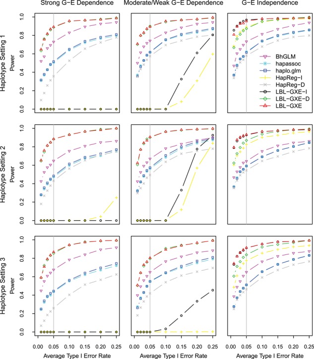
Power for detecting the interaction effect in Scenario 1. The simulation scenarios are described in Table 3.
Figure 3.

Power for detecting the main haplotype effect in Scenario 1. The simulation scenarios are described in Table 3.
Simulations based on the lung cancer data
To further examine the methods under realistic linkage disequilibrium patterns, we generate four simulation scenarios based on the lung cancer data (described in the next section). We simulate data in a similar manner as in the above simulations; however, we use the haplotypes and their frequencies (estimated separately for smokers and non-smokers) estimated from the lung cancer data as shown in Table 4. We also simulate smoking as a covariate with 83% prevalence for smokers to mimic the real data. Following Zhang et al. [26], three scenarios are constructed by using the estimated ORs corresponding to the significant effects of smoking and interactions obtained from our lung cancer data analysis reported in the next section (in Table 5) (Scenario 1) and their variations (Scenarios 2 and 3). Additionally, we also consider a completely null scenario (Scenario 0). The details of these four scenarios are shown in Table 4. The sample size is 5000 with equal numbers of cases and controls (similar to the real data). For each scenario, we run 500 replicates. The haplotype h10 is used as the baseline. In some replicates, haplotypes other than h1 through h10, which were used in the simulation model, were estimated by one or more methods and we denote them as hOth. The results are shown in Figure 4. HapReg did not converge in any replicate and hapassoc also did not converge for about 96–99% replicates, and thus we do not report results for these two methods. Haplo.glm converged in 93–97% replicates (due to its pooling tolerance being 0.001 rather than 0); however, as seen in Figure 4, it has uncontrollably high type I error rates. BhGLM also has few slightly inflated type I error rates as seen in Scenarios 2 (for h9) and 3 (for h4). So, even though it has slightly higher power than LBL for detecting the rare haplotype interaction, adjusting the cutoff to make the false-positive rates the same may possibly decrease the apparently increased power of BhGLM. Similarly, LBL-GXE-I has also few inflated type I error rates (e.g. for h8 in Scenario 0) as G–E independence does not hold in these data [26].
Table 4.
Models for lung cancer data-based simulation. An ‘*’ indicates interaction effect of the corresponding haplotype with E.
| Haplotype | Association scenarios (OR) | Frequency | ||||
|---|---|---|---|---|---|---|
| 0 | 1 | 2 | 3 |

|

|
|
| h1: 1110 | – | – | – | – | 0.0005 | 0 |
| h2: 1100 | – | – | – | – | 0.126 | 0.1247 |
| h3: 1010 | – | – | – | – | 0 | 0.0016 |
| h4: 1001 | – | – | – | 5* | 0.0054 | 0.0025 |
| h5: 1000 | – | 1.40* | 1.5* | 1.5* | 0.2694 | 0.2788 |
| h6: 0100 | – | – | – | – | 0.0032 | 0.0017 |
| h7: 0011 | – | – | – | – | 0 | 0.0002 |
| h8: 0010 | – | – | – | – | 0.2277 | 0.208 |
| h9: 0000 | – | 2.14* | 3* | – | 0.0119 | 0.0154 |
| h10: 0001 | – | – | – | – | 0.3559 | 0.3671 |
| E | – | 2.78 | 2 | 2 | – | – |
Table 5.
Results of lung cancer data analysis for three blocks showing significant haplotype–smoking interactions. Significant results are shown in bold.
| Haplotype block | SNP | Haplotypes | ||||
|---|---|---|---|---|---|---|
| Block 1 | rs1394371 | C | ||||
| rs12903150 | A | |||||
| rs12899131 | G | |||||
| rs2656069 | A | |||||
| Block 2 | rs13180 | C | ||||
| rs3743079 | T | |||||
| Block 3 | rs8034191 | C | T | |||
| rs3885951 | T | T | ||||
| rs2036534 | T | T | ||||
| rs2292117 | G | G | ||||
| Block 4 | rs12914385 | T | ||||
| rs1051730 | T | |||||
| rs1948 | C | |||||
| Hap Freq | 0.17 | 0.17 | 0.28 | 0.01 | 0.40 | |
| LBL-GXE OR | 0.74 | 0.81 | 1.40 | 2.14 | 0.76 | |
| LBL-GXE 95% CS LB | 0.54 | 0.59 | 1.09 | 0.98 | 0.60 | |
| LBL-GXE 95% CS UB | 1.02 | 1.06 | 1.83 | 5.70 | 0.99 | |
| LBL-GXE BF | 0.83 | 0.81 | 2.94 | 2.42 | 0.96 | |
| Interaction effects with smoking | LBL-GXE-D OR | 0.74 | 0.75 | 1.40 | 2.16 | 0.76 |
| LBL-GXE-D 95% CS LB | 0.54 | 0.54 | 1.07 | 0.99 | 0.58 | |
| LBL-GXE-D 95% CS UB | 0.99 | 1.01 | 1.84 | 5.55 | 0.98 | |
| LBL-GXE-D BF | 1.01 | 0.79 | 2.16 | 2.63 | 0.97 | |
| haplo.glm OR | 0.63 | 0.68 | 1.48 | 2.81 | 0.72 | |
haplo.glm  -value -value |
0.01 | 0.02 | 0.01 | 0.07 | 0.02 | |
| BhGLM OR | 0.73 | 0.75 | 1.37 | 1.87 | 0.75 | |
BhGLM  -value -value |
0.03 | 0.05 | 0.02 | 0.03 | 0.02 |
Hap Freq, haplotype frequency (as estimated by hapassoc); LB, lower bound; UB, upper bound
Figure 4.

Powers (in gray shadow) and type I error rates for simulations based on the lung cancer data. The four scenarios are described in Table 4. HOth represents haplotypes other than those listed in the table when estimated by a model. Each plot has two panels for main effects (bottom) and interactions of the corresponding haplotypes with E (top).
Application to the lung cancer data
We apply all methods to the lung cancer GWAS data collected in the Environment And Genetics in Lung cancer Etiology study and the Prostate, Lung, Colorectal and Ovarian Cancer Screening Trial. The total sample size is 5549 with 2728 cases and 2821 controls. We focus on region 15q25.1 as variants in this region have been implicated to interact with smoking in affecting lung cancer risk [26, 33–36]. Moreover, this region has been shown to be associated with smoking behavior rendering G–E independence assumption untenable [33, 37–39]. Thus, this region serves as an excellent test region for comparing the GXE methods. Further, availability of a reasonably large sample provides us with an opportunity to study potential interaction effects of smoking with rare haplotypes.
Following Zhang et al. [26], we consider five haplotype blocks in this region as obtained from Haploview [40] using these data: (i) Block 1 with four SNPs: rs1394371, rs12903150, rs12899131 and rs2656069; (ii) Block 2 with two SNPs: rs13180 and rs3743079; (iii) Block 3 with four SNPs: rs8034191, rs3885951, rs2036534 and rs2292117; (iv) Block 4 with three SNPs: rs12914385, rs1051730 and rs1948; and (v) Block 5 with 2 SNPs: rs11636753 and rs12441998. We analyze each block separately with each analysis model consisting of the main effects of haplotypes and smoking and their interaction effects. To ensure convergence of MCMC algorithm in LBL methods in presence of rare haplotypes, following Zhang et al. [26], the total number of MCMC iterations were set to 800 000 with a burn-in of 400 000. Due to presence of several rare haplotypes, hapassoc and HapReg did not converge in any block. BhGLM, haplo.glm and LBL found few significant interactions as reported in Table 5 along with an extremely strong main effect of smoking. In particular, BhGLM and LBL found a significant interaction effect of smoking with rare haplotype TTTG in Block 3. No main effect of any haplotype was detected. Thus, smokers who are carriers of TTTG haplotype have about two times higher odds of lung cancer than smokers with the baseline haplotype.
Application to the DHS data
DHS is a population-based study with sequence data collected on 3 ethnicities—African Americans (n = 1832), European Americans (n = 1043) and Hispanic (n = 601) [28]. The gene ANGPTL4 has been implicated to be associated with trait serum triglyceride (TG) [41–43]. While African Americans, in general, have lower TG levels than Whites [44, 45], European Americans with a specific non-synonymous sequence variant E40K in the ANGPTL4 tend to have lower TG levels [43]. Even though most genetic studies adjust for race in their models, no study of this gene has explicitly investigated interactions with race, at least to the best of our knowledge. As our focus is on detecting interactions, we decided to explore interactions with race using the GXE methods considered in the present study.
Following several previous studies, we use a dichotomized version of TG [12, 13, 46]. Although most studies use top 20% and bottom 20% TG values as cases and controls, respectively, we extend the criterion to include top 40% (cases) and bottom 40% (controls) to retain a larger sample size, which is necessary to have some power to detect interactions, especially due to presence of extremely rare haplotypes (some of the order  0.0001). On applying this criterion and excluding subjects treated with statin [13, 46], we have a sample size of 2512 with 1261 cases and 1251 controls. Of these, 746, 1307 and 459 are Whites, Blacks and Hispanics, respectively. Among the variant types, we included missense substitutions, nonsense substitutions and frameshift insertions and deletions to get a total of 19 variants on this gene [13, 46].
We analyzed these variants through sliding windows (haplotype blocks) of five variants. That is, variants 1–5, 2–6, 3–7 and so on to form 15 blocks (windows). Race is used as a covariate, i.e. it is used as E in the models even though it is not an environmental factor as such rather it is a non-genetic factor. We use Whites as the baseline. All interaction terms of race with haplotypes are included in the model for each block. To ensure convergence of LBL methods in presence of rare haplotypes, the total number of MCMC iterations were set to 200000 iterations with a burn-in of 100 000. As in the lung cancer data analyses, hapassoc and HapReg did not converge. In all windows, a strong main effect of race was found with Blacks having OR < 1 (BhGLM’s  -values
  0 and LBL’s BF > 100). In some windows, the main effect for Hispanics was significant with OR > 1 but this effect was relatively weaker. BhGLM did not find any significant interaction effects. LBL-GXE-D and LBL-GXE found few significant interactions as reported in Table 6, which show that Hispanics with the reported haplotypes have increased odds of being a case (elevated TG). However, these signals are weak because even though the 95% CS for OR technically excludes 1, the lower limit is practically 1 and the BF is small. This is expected due to a relatively small sample size and more rarity of the haplotypes in DHS compared to the lung cancer data analyzed earlier.
Table 6.
Results of DHS for two blocks showing significant haplotype–race interactions. Significant results are shown in bold.
| Haplotypes | |||
|---|---|---|---|
| Window 8 | Window 9 | ||
| SNPs | 8020_P251T | 0 | |
| 8155_T266M | 1 | 1 | |
| 8191_R278Q | 0 | 0 | |
| 8262_S302fs | 0 | 0 | |
| 8277_P307S | 0 | 0 | |
| 8280_V308M | 0 | ||
| Freq | 0.2643 | 0.2645 | |
| LBL-GXE OR | 1.4045 | 1.3774 | |
| LBL-GXE 95% CS LB | 1.0102 | 0.9913 | |
| Interaction effects with race (Hispanic) | LBL-GXE 95% CS UB | 1.9485 | 1.9329 |
| LBL-GXE BF | 1.2351 | 1.0017 | |
| LBL-GXE-D OR | 1.4001 | 1.3941 | |
| LBL-GXE-D 95% CS LB | 1.0111 | 1.0022 | |
| LBL-GXE-D 95% CS UB | 1.9473 | 1.9447 | |
| LBL-GXE-D BF | 1.2401 | 1.1283 | |
LBL-GXE-I and haplo.glm found several interaction effects to be significant; however, these are quite likely to be false positives and thus we do not report them individually. The BFs given by LBL-GXE-I are mostly extreme (exceeding 100) raising doubts about their reliability. This is especially because it has been shown that LBL-GXE-I has high type I error rates when G–E independence assumption is violated [26] and this was also confirmed in our earlier simulation results. For the DHS data, G–E independence assumption clearly does not hold because frequencies of haplotype (G) depends on race (E). Note that the haplotype frequencies reported in Table 6 are estimated by the hapassoc for the overall sample including all three races. In fact, the estimated frequencies do vary by races when each race is analyzed separately by hapassoc (results not shown). For haplo.glm, the  -values of significant interaction effects are all zero, and the estimated standard errors are also practically zero suggesting the results are unreliable.
Discussion
Detecting rare variants and GXE are of great scientific interest currently due to their potential to explain missing heritability. Thus, a highly relevant and timely question is how haplotype-based tests perform in terms of their powers to detect GXE with G being a rare haplotype. To answer this question, we studied five haplotype association tests including two versions of HapReg and three versions of LBL leading to a total of eight different methods. For a robust and unbiased assessment, we applied the methods to two different types of real data sets, one consisting of GWAS data and another of sequence data, and to simulated data under a wide variety of settings including those based on the lung cancer data.
In our simulations, we found that haplo.glm can have uncontrollably high type I error rates, relatively to the nominal level, in presence of rare haplotypes as seen in lung cancer data-based simulations. Also, LBL-GXE-I and HapReg-I gave extremely inflated false-positive rates when G–E independence assumption was not satisfied. Unexpectedly, HapReg-D was unable to control type I error rate under strong G–E dependence even though that version was specifically devised to handle G–E dependence. In fact, HapReg as well as hapassoc did not even converge in presence of extremely rare haplotypes making them unviable options in such situations.
As not all methods maintained type I error rates consistent with the nominal levels, we relied on the empirical ROC curves in order to make valid power comparisons. Among all methods studied, HapReg-I and LBL-GXE-I appeared to have very low power for detecting GXE interactions, unless G–E independence holds, as expected. Generally, HapReg-D had the lowest power for detecting GXE regardless of whether G–E independence holds or not. On the other hand, LBL-GXE consistently had the highest power, in some cases increasing the power by about 20% in absolute scale when compared to the 2nd best method, BhGLM (not considering LBL-GXE-D).
Although not the direct focus of this study, we also examined the power to detect main haplotype effect. In this regard also, we found LBL to perform the best unless the haplotype is common, in which case BhGLM has higher power than LBL, especially under G–E dependence. Thus, in summary, we may conclude that if the interest lies in detecting rare haplotypes, be it main or interaction effect, LBL appears to be the method of choice among the methods considered here.
One practical issue related to the use of LBL is whether BF or CS should be used for inference. Both control type I error rate reasonably well in general. However, in some G–E dependence scenarios, BF may give slightly higher false-positive rate (e.g. see Supplementary Table 1) while in some situations, it can be conservative [47]. As an example of the latter, in the DHS analyses, we could detect significant interactions using CS criterion only. Thus, for real data applications, we recommend reporting both CS and BF. The two will typically lead to similar inference if the signal is strong. Another issue is whether LBL can handle very rare haplotypes. In our both real data analyses as well as the simulations based on the lung cancer data, there were some extremely rare haplotypes with frequencies of the order of 0.0001–0.001. LBL appears to handle those well with the available sample sizes. Nonetheless, in presence of very rare haplotypes, Zhang et al. [26] strongly recommend monitoring convergence of the Markov chain. If needed, increasing the number of iterations can help achieve satisfactory convergence (as we did in our real data analyses).
A disadvantage of LBL is its computational intensity, which being MCMC-based, exceeds that of other methods substantially. For the analysis of a simulated replicate from simulation association scenario 1, haplotype setting 1, with strong G–E dependence, the time needed to complete the analysis for LBL-GXE, LBL-GXE-D and LBL-GXE-I were 521, 504 and 247 s while the corresponding times for hapassoc, haplo.glm and BhGLM were 4, 1 and 1.4 s, respectively. These computing times are for a 2.40 GHz Xeon processor under Linux operating system with 8 GB RAM. For HapReg, we had to run its SAS code on a Windows machine (as its Linux version did not work), and thus its computing time is not comparable with those of others mentioned above. As LBL-GXE is the most computationally intensive of the three versions of LBL, Zhang et al. [26] suggest that LBL-GXE-I (or LBL-GXE-D) can be used in scenarios where it is known beforehand that G–E independence holds (or does not hold). However, they show through simulations that it is not optimal to use a two-stage approach wherein a test of G–E independence is first carried out and then accordingly a specific version is chosen and applied.
When applied to the lung cancer GWAS data, BhGLM, LBL-GXE-D and LBL-GXE were the only methods that identified an interaction effect of smoking with a rare haplotype TTTG. In the DHS sequence data, only LBL-GXE and LBL-GXE-D detected interaction effects of race (Hispanic) with two haplotypes, albeit both being common. Even though the results were not highly significant (likely due to the small sample size of the sequence data), they may be useful for follow-up studies with larger sample sizes. Haplo.glm and LBL-GXE-I found numerous significant interactions in DHS; however, we believe those results may be unreliable as the corresponding  -values and BFs were extreme, and because our simulations suggested a propensity of high false-positive rates by haplo.glm and LBL-GXE-I in presence of rare haplotypes and G–E dependence, respectively.
A useful and relevant future work is to make LBL more computationally efficient. Another interesting work will be to compare the family-based association methods for detecting rare haplotypes and their interactions as well as comparing those methods with their population-based counterparts, particularly under population sub-structure as in [12]. Similarly, comparing haplotype methods (population based as well as family based) for detecting association with quantitative traits will be also helpful for practitioners.
WEB RESOURCES
The URLs for software packages are as follows:
hapassoc: http://stat-db.stat.sfu.ca:8080/~statgen/research/hapassoc
haplo.glm: http://www.mayo.edu/research/labs/statistical-genetics-genetic-epidemiology/software
Data simulation code: https://github.com/babinetos/SimHaplos
Key Points
Several haplotype association methods have been proposed recently for detecting GXE with rare variants.
We compared eight haplotype association methods—haplo.glm, hapassoc, HapReg (two versions), BhGLM and LBL (three versions)—in terms of their power to detect GXE through extensive simulations and real data analyses.
The most powerful method for detecting GXE is a version of LBL that allows for uncertainty in G–E independence assumption.
Supplementary Material
Funding
National Cancer Institute (R03CA171011).
Charalampos Papachristou is an associate professor of statistics at the Rowan University.
Swati Biswas is a professor of statistics in the Department of Mathematical Sciences at the University of Texas at Dallas.
Acknowledgments
We thank Drs. Jonathan Cohen and Helen Hobbs for providing the DHS data. The lung cancer data set was obtained through dbGaP accession number phs000093.v2.p2. We thank the anonymous reviewers for providing constructive comments, which led to an improved version of the paper.
References
- 1. Thomas D. Gene–environment-wide association studies: emerging approaches. Nat Rev Genet 2010;11:259–272. [DOI] [PMC free article] [PubMed] [Google Scholar]
- 2. Maher B. Personal genomes: the case of the missing heritability. Nature 2008; 456:18–21. [DOI] [PubMed] [Google Scholar]
- 3. Manolio TA, Collins FS, Cox NJ, et al. Finding the missing heritability of complex diseases. Nature 2009;461:747–753. [DOI] [PMC free article] [PubMed] [Google Scholar]
- 4. Basu S, Pan W. Comparison of statistical tests for disease association with rare variants. Genet Epidemiol 2011;35:606–619. [DOI] [PMC free article] [PubMed] [Google Scholar]
- 5. Li Y, Byrnes AE, Li M. To identify associations with rare variants, just WHaIT: weighted haplotype and imputation-based tests. Am J Hum Genet 2010;87:728–735. [DOI] [PMC free article] [PubMed] [Google Scholar]
- 6. Lin WY, Yi N, Zhi D, et al. Haplotype-based methods for detecting uncommon causal variants with common SNPs. Genet Epidemiol 2012;36:572–582. [DOI] [PMC free article] [PubMed] [Google Scholar]
- 7. Guo W, Lin S. Generalized linear modeling with regularization for detecting common disease rare haplotype association. Genet Epidemiol 2009;33:308–316. [DOI] [PMC free article] [PubMed] [Google Scholar]
- 8. Biswas S, Lin S. Logistic Bayesian LASSO for identifying association with rare haplotypes and application to age-related macular degeneration. Biometrics 2012;68:587–597. [DOI] [PubMed] [Google Scholar]
- 9. Li J, Zhang K, Yi N. A Bayesian hierarchical model for detecting haplotype–haplotype and haplotype–environment interactions in genetic association studies. Hum Hered 2011;71:148–160. [DOI] [PMC free article] [PubMed] [Google Scholar]
- 10. Lin WY, Yi N, Lou XY, et al. Haplotype kernel association test as a powerful method to identify chromosomal regions harboring uncommon causal variants. Genet Epidemiol 2013;37:560–570. [DOI] [PMC free article] [PubMed] [Google Scholar]
- 11. Dering C, Hemmelmann C, Pugh E, Ziegler A. Statistical analysis of rare sequence variants: an overview of collapsing methods. Genet Epidemiol 2011;35(Suppl 1): S12–S17. [DOI] [PMC free article] [PubMed] [Google Scholar]
- 12. Wang M, Lin S. Detecting associations of rare variants with common diseases: collapsing or haplotyping? Brief Bioinform 2015;16:759–768. [DOI] [PMC free article] [PubMed] [Google Scholar]
- 13. Datta AS, Biswas S. Comparison of haplotype-based statistical tests for disease association with rare and common variants. Brief Bioinform 2016;17:657–671. [DOI] [PMC free article] [PubMed] [Google Scholar]
- 14. Goldstein DB, Allen A, Keebler J, et al. Sequencing studies in human genetics: design and interpretation. Nat Rev Genet 2013;14:460–470. [DOI] [PMC free article] [PubMed] [Google Scholar]
- 15. Schaid DJ, Rowland CM, Tines DE, et al. Score tests for association between traits and haplotypes when linkage phase is ambiguous. Am J Hum Genet 2002;70:425–434. [DOI] [PMC free article] [PubMed] [Google Scholar]
- 16. Schaid DJ. Genetic epidemiology and haplotypes. Genet Epidemiol 2004;27:317–320. [DOI] [PubMed] [Google Scholar]
- 17. Morris RW, Kaplan NL. On the advantage of haplotype analysis in the presence of multiple disease susceptibility alleles. Genet Epidemiol 2002;23:221–233. [DOI] [PubMed] [Google Scholar]
- 18. Chen YH, Chatterjee N, Carroll RJ. Retrospective analysis of haplotype-based case-control studies under a flexible model for gene–environment association. Biostatistics 2008;9:81–99. [DOI] [PMC free article] [PubMed] [Google Scholar]
- 19. Chen YH, Chatterjee N, Carroll RJ. Shrinkage estimators for robust and efficient inference in haplotype-based case-control studies. J Am Stat Assoc 2009;104:220–233. [DOI] [PMC free article] [PubMed] [Google Scholar]
- 20. Burkett K, McNeney B, Graham J. A note on inference of trait associations with SNP haplotypes and other attributes in generalized linear models. Hum Hered 2004;57:200–206. [DOI] [PubMed] [Google Scholar]
- 21. Burkett K, Graham J, McNeney B. Hapassoc: software for likelihood inference of trait associations with SNP haplotypes and other attributes. J Stat Softw 2006;16:1–19. [Google Scholar]
- 22. Lake SL, Lyon H, Tantisira K, et al. Estimation and tests of haplotype–environment interaction when linkage phase is ambiguous. Hum Hered 2003;55:56–65. [DOI] [PubMed] [Google Scholar]
- 23. Datta AS, Zhang Y, Zhang L, Biswas S. Association of rare haplotypes on ULK4 and MAP4 genes with hypertension. BMC Proc 2015;10(Suppl 7): 44. [DOI] [PMC free article] [PubMed] [Google Scholar]
- 24. Biswas S, Xia S, Lin S. Detecting rare haplotype–environment interaction with logistic Bayesian LASSO. Genet Epidemiol 2014;38:31–41. [DOI] [PMC free article] [PubMed] [Google Scholar]
- 25. Zhang Y, Biswas S. An improved version of logistic Bayesian LASSO for detecting rare haplotype–environment interactions with application to lung cancer. Cancer Inform 2015;14(S2): 11–16. [DOI] [PMC free article] [PubMed] [Google Scholar]
- 26. Zhang Y, Lin S, Biswas S. Detecting rare and common haplotype–environment interaction under uncertainty of gene–environment independence assumption. Biometrics 2017;73:344–355. [DOI] [PMC free article] [PubMed] [Google Scholar]
- 27. Lung Cancer GWAS Data. https://www.ncbi.nlm.nih.gov/projects/gap/cgi-bin/study.cgi?study_id=phs000093.v2.p2. ( 3 December 2018, date last accessed).
- 28. Victor RG, Haley RW, Willett DL, et al. The Dallas Heart Study: a population-based probability sample for the multidisciplinary study of ethnic differences in cardiovascular health. Am J Cardiol 2004;93:1473–1480. [DOI] [PubMed] [Google Scholar]
- 29. Prentice RL, Pyke R. Logistic disease incidence models and case-control studies. Biometrika 1979;66:403–411. [Google Scholar]
- 30. Epstein MP, Satten GA. Inference on haplotype effects in case-control studies using unphased genotype data. Am J Hum Genet 2003;73:1316–1329. [DOI] [PMC free article] [PubMed] [Google Scholar]
- 31. Satten GA, Epstein MP. Comparison of prospective and retrospective methods for haplotype inference in case-control studies. Genet Epidemiol 2004;27:192–201. [DOI] [PubMed] [Google Scholar]
- 32. Chatterjee N, Carroll RJ. Semiparametric maximum likelihood estimation exploiting gene–environment independence in case-control studies. Biometrika 2005;92:399–418. [Google Scholar]
- 33. Thorgeirsson TE, Geller F, Sulem P, et al. A variant associated with nicotine dependence, lung cancer and peripheral arterial disease. Nature 2008;452:638–642. [DOI] [PMC free article] [PubMed] [Google Scholar]
- 34. Yokota J, Shiraishi K, Kohno T. Genetic basis for susceptibility to lung cancer: recent progress and future directions. Adv Cancer Res 2010;109:51–72. [DOI] [PubMed] [Google Scholar]
- 35. Yu K, Wacholder S, Wheeler W, et al. A flexible Bayesian model for studying gene–environment interaction. PLoS Genet 2012;8:e1002482. [DOI] [PMC free article] [PubMed] [Google Scholar]
- 36. VanderWeele TJ, Asomaning K, Tchetgen Tchetgen EJ, et al. Genetic variants on 15q25.1, smoking, and lung cancer: an assessment of mediation and interaction. Am J Hum Genet 2012;175:1013–1020. [DOI] [PMC free article] [PubMed] [Google Scholar]
- 37. Spitz MR, Amos CI, Dong Q, et al. The CHRNA5-A3 region on chromosome 15q24-25.1 is a risk factor both for nicotine dependence and for lung cancer. J Nat Cancer Inst 2008;100:1552–1556. [DOI] [PMC free article] [PubMed] [Google Scholar]
- 38. Saccone NL, Culverhouse RC, Schwantes-An TH, et al. Multiple independent loci at chromosome 15q25.1 affect smoking quantity: a meta-analysis and comparison with lung cancer and COPD. PLoS Genet 2010;6:e1001053. [DOI] [PMC free article] [PubMed] [Google Scholar]
- 39. Liu JZ, Tozzi F, Waterworth DM, et al. Meta-analysis and imputation refines the association of 15q25 with smoking quantity. Nat Genet 2010;42:436–440. [DOI] [PMC free article] [PubMed] [Google Scholar]
- 40. Barrett JC, Fry B, Maller J, Daly MJ. Haploview: analysis and visualization of LD and haplotype maps. Bioinformatics 2005;21:263–265. [DOI] [PubMed] [Google Scholar]
- 41. Romeo S, Yin W, Kozlitina J, et al. Rare loss-of-function mutations in ANGPTL family members contribute to plasma triglyceride levels in humans. J Clin Invest 2009;119:70–79. [DOI] [PMC free article] [PubMed] [Google Scholar]
- 42. Mehta N, Qamar A, Qu L, et al. Differential association of plasma angiopoietin-like proteins 3 and 4 with lipid and metabolic traits. Arterioscler Thromb Vasc Biol 2014;34:1057–1063. [DOI] [PMC free article] [PubMed] [Google Scholar]
- 43. Romeo S, Pennacchio LA, Fu Y, et al. Population-based resequencing of ANGPTL4 uncovers variations that reduce triglycerides and increase HDL. Nat Genet 2007;39:513–516. [DOI] [PMC free article] [PubMed] [Google Scholar]
- 44. Lin SX, Carnethon M, Szklo M, Bertoni A.. Racial/ethnic differences in the association of triglycerides with other metabolic syndrome components: the Multi-Ethnic Study of Atherosclerosis. Metab Syndr Relat Disord 2011;9:35–40. [DOI] [PMC free article] [PubMed] [Google Scholar]
- 45. McIntosh MS, Kumar V, Kalynych C, et al. Racial differences in blood lipids lead to underestimation of cardiovascular risk in black women in a nested observational study. Glob Adv Health Med 2013;2:76–79. [DOI] [PMC free article] [PubMed] [Google Scholar]
- 46. Turkmen AS, Yan Z, Hu YQ, Lin S. Kullback–Leibler distance methods for detecting disease association with rare variants from sequencing data. Ann Hum Genet 2015;79:199–208. [DOI] [PubMed] [Google Scholar]
- 47. Datta AS, Lin S, Biswas S. A family-based rare haplotype association method for quantitative traits. Hum Hered 2018;83:175–195. [DOI] [PMC free article] [PubMed] [Google Scholar]
- 48. Zhang H. Detecting rare haplotype–environmental interaction and nonlinear effects of rare haplotypes using Bayesian LASSO on quantitative traits.. PhD diss., The Ohio State University, 2017. https://etd.ohiolink.edu/pg_10?0::NO:10:P10_ETD_SUBID:151733. [Google Scholar]
Associated Data
This section collects any data citations, data availability statements, or supplementary materials included in this article.