Abstract
We present a fractional-order model for the COVID-19 transmission with Caputo–Fabrizio derivative. Using the homotopy analysis transform method (HATM), which combines the method of homotopy analysis and Laplace transform, we solve the problem and give approximate solution in convergent series. We prove the existence of a unique solution and the stability of the iteration approach by using fixed point theory. We also present numerical results to simulate virus transmission and compare the results with those of the Caputo derivative.
Keywords: Fixed point, Homotopy analysis method, Mathematical model, Numerical simulation, Caputo–Fabrizio derivative
Introduction
Corona viruses are a large family of viruses that have a distinctive corona or ‘crown’ of sugary-proteins, and because of their appearance, they were called corona viruses in 1960. Viruses that cause common cold diseases and fatal diseases, such as Middle East respiratory syndrome (MERS-CoV) and severe acute respiratory syndrome (SARS-CoV), are from the corona viruses family. Detailed investigations found that corona viruses are transmitted between animals and people, for instance, SARS-CoV and MERS-CoV were transmitted from civet cats and dromedary camels to humans, respectively. Also, several known corona viruses that have not yet infected humans are circulating in animals.
COVID-19, which was first identified in the Wuhan city, is a new strain that has not been previously identified in humans. Snakes or bats have been suspected as a potential source for the outbreak, though other experts currently consider this unlikely. Fever, cough, shortness of breath, and breathing difficulties are the initial symptoms of this infection. In the next steps, the infection can cause pneumonia, severe acute respiratory syndrome, kidney failure, and even death.
The study of disease dynamics is a dominating theme for many biologists and mathematicians (see, for example, [1–10]). It has been studied by many researchers that fractional extensions of mathematical models of integer order represent the natural fact in a very systematic way such as in the approach of Akbari et al. [11], Baleanu et al. [12–24], and Talaee et al. [25]. In this paper, we use the new fractional Caputo–Fabrizio derivative [26] to express the mathematical modeling for simulating the transmission of COVID-19. Recently, many works related to the fractional Caputo–Fabrizio derivative have been published (see, for example, [21, 23, 24, 27–30]). The Caputo–Fabrizio fractional derivative is also used to study the dynamics of diseases (see, for example, [31–34]). Mathematical models are used to simulate the transmission of corona virus (see, for example, [35, 36]). A mathematical model for the transmission of COVID-19 was presented by Chen et al. [37]. In this work, we investigate this model by using the Caputo–Fabrizio fractional derivative.
Now, we recall some fundamental notions. The Caputo fractional derivative of order η for a function f via integrable differentiations is defined by , where . Our second notion is a fractional derivative without singular kernel which was introduced by Caputo and Fabrizio in 2015 [26]. Let , , and . The Caputo–Fabrizio derivative of order η for a function f is defined by
where , is a normalization function that depends on η and . If and , this derivative can be presented for as
(see [38]). Let and . The fractional derivatives of order are defined by [28]. The Laplace transform of the Caputo–Fabrizio derivative is defined by , where and [38].
The Riemann–Liouville fractional integral of order η with is defined by [28]. The fractional integral of Caputo–Fabrizio is defined by () [38]. The Sumudu transform is derived from the classical Fourier integral ([39–41]). Consider the set
The Sumudu transform of a function is defined by
for all , and the inverse Sumudu transform of is denoted by [40]. The Sumudu transform of the Caputo derivative is given by
where () [39]. Let F be a function such that its Caputo–Fabrizio fractional derivation exists. The Sumudu transform of F with Caputo–Fabrizio fractional derivative is defined by [42].
A mathematical model for the transmission of COVID-19 with Caputo–Fabrizio fractional derivative
Chen and colleagues have proposed a transmission network model to simulate possible transmission from the source of infection (possibly bats) to human infection [37]. They assumed that the virus was transmitted among the bats’ population, and then transmitted to an unknown host (probably wild animals). Then hosts were hunted and sent to the seafood market, which was defined as the reservoir or the virus. People exposed to the market got the risks of the infection. In the presented model, people were divided into five groups: susceptible people (S), exposed people (E), symptomatic infected people (I), asymptomatic infected people (A), and removed people (R) including recovered and dead people. COVID-19 in the reservoir was denoted as (W). This model was presented as follows:
where
, N refer to the total number of people and n is the birth rate,
m: the death rate of people,
: the transmission rate from I to S,
κ: the multiple of the transmissible of A to that of I,
: the transmission rate from W to S,
δ: the proportion of asymptomatic infection rate of people
: the incubation period of people,
: the latent period of people,
: the infectious period of symptomatic infection of people,
: the infectious period of asymptomatic infection of people,
μ: the shedding coefficients from I to W,
: the shedding coefficients from A to W,
: the lifetime of the virus in W.
Also, the initial conditions are , , , , .
We moderate the system by substituting the time derivative by the Caputo–Fabrizio fractional derivative in the Caputo sense [26]. With this change, the right- and left-hand sides will not have the same dimension. To solve this problem, we use an auxiliary parameter ρ, having the dimension of sec., to change the fractional operator so that the sides have the same dimension [43]. According to the explanation presented, the COVID-19 transmission fractional model for and is given as follows:
| 1 |
where the initial conditions are , , , , . In the next section we investigate the existence and uniqueness of the solution for system (1) by fixed point theorem.
Existence of a unique solution
In this section, we show that the system has a unique solution. For this purpose, employing the fractional integral operator due to Nieto and Losada [38] on the system (1), we obtain
Using the definition of Caputo–Fabrizio fractional integral [38], we obtain
| 2 |
For convenience, we consider
Theorem 3.1
The kernelsatisfies the Lipschitz condition and contraction if the following inequality holds:
Proof
Consider functions and , then
Let , where and are bounded functions, then we have
Thus, the Lipschitz condition is fulfilled for . In addition, if , then is a contraction. □
Similarly, , , , , satisfy the Lipschitz condition as follows:
On consideration of , , , , , , we can write equation (2) as follows:
Thus, consider the following recursive formula:
where , , , , , .
Now, we consider
Given the above equations, one can write
| 3 |
According to ’s definition and using the triangular inequality, we have
satisfies the Lipschitz condition, therefore
Thus we get
| 4 |
It can be shown that similar results are obtained for , as follows:
| 5 |
According to the above result, we show that system (1) has a solution.
Theorem 3.2
The fractional COVID-19 model (1) has a system of solutions if there exist, , such that
Proof
Assume that functions , , , , , are bounded. We have shown that kernels , satisfy the Lipschitz condition. By using the recursive method and the results of (4) and (5), we obtain
Thus, functions (3) exist and are smooth. We claim that the above functions are the solutions of system (1). To prove this claim, we assume
We have
By repeating this process, we obtain
By taking limit on recent equation as n tends to infinity, we obtain . By the same way, we get , , and this completes the proof. □
To prove the uniqueness of solution, we assume that system (1) has another solution such as , , , , , . Then
According to the Lipschitz condition of S, we get
Thus
| 6 |
Theorem 3.3
The solution of COVID-19 fractional model (1) is unique if the following condition holds:
| 7 |
Proof
From condition (7) and equation (6), we conclude that
So , then . In the same way, we can show that
The proof is complete. □
Stability analysis by fixed point theory
Using the Sumudu transform, we obtain a special solution to the COVID-19 model and then prove the stability of the iterative method using fixed point theory. At first, we apply the Sumudu transform on both sides of equations in model (1), then
We conclude from the Sumudu transform definition of the Caputo–Fabrizio derivative the following:
If we rearrange the above inequalities, then
We obtain
| 8 |
The approximate solution of system (1) is as follows:
Stability analysis of iteration method
Consider the Banach space , a self-map T on G, and the recursive method . Assume that is the fixed point set of T which and . Suppose that and . If implies that , then the recursive procedure is T-stable. Suppose that our sequence has an upper boundary. If Picard’s iteration is satisfied in all these conditions, then is T-stable.
Theorem 4.1
([44])
Letbe a Banach space andTbe a self-map ofGsatisfying
for allwhereand. Suppose thatTis PicardT-stable.
According to (8), the fractional model of COVID-19 (1) is connected with the subsequent iterative formula. Now consider the following theorem.
Theorem 4.2
Suppose thatTis a self-map defined as follows:
This iterative recursive isT-stable inif the following conditions are achieved:
Proof
To prove that T has a fixed point, we compute the following inequalities for :
By applying norm on both sides, we obtain
| 9 |
Since the solutions have the same roles, we can consider
| 10 |
From equations (9) and (10), we get
| 11 |
, , , , , are bounded because they are convergent sequences, then for all t there exist , , such that
| 12 |
From equations (11) and (12), we get
| 13 |
where are functions from . Similarly, we will obtain
| 14 |
where
Thus the T-self mapping has a fixed point. Also, we show that T satisfies the conditions in Theorem 4.1. Consider that (13), (14) hold, we assume
So, all the conditions of Theorem 4.1 are satisfied and the proof is complete. □
Numerical method
In this section, we apply the homotopy analysis transform method (HATM) to implement the fractional model (1) appropriately. Notice that HATM is a well-developed mixture of the standard Laplace transform technique [45] and the homotopy analysis method (HAM) [46]. To solve model (1) by HATM, first we apply the Laplace transform in the following way:
which results in
Then we get
| 15 |
Using the homotopy method, we define
Then the deformation equations become
where denotes an embedding parameter; , , are unknown functions; , , , , , are initial guesses; is the Laplace operator; is an auxiliary function, and is a nonzero auxiliary parameter. Clearly, for and , we have
Thus, increasing q from zero to one varies the solution from to . Now, we expand () in the Taylor series with regard to q. This procedure yields
where
| 16 |
If the auxiliary function , the auxiliary parameter h, and the initial guesses are properly chosen, then series (16) converges at , as proved by Liao [46]. Thus, we get
In addition, we can express the mth order deformation equation by
| 17 |
where
| 18 |
and
Applying the inverse Laplace transform to equation (17), we obtain
Solving these equations for different values of , we derive
where
Finally, the solutions of system (1) are obtained as follows:
Convergency of HATM for FDEs
In the following, we discuss the convergence of HATM by presenting and proving the following theorem.
Theorem 5.1
Let, , , , , andbe uniformly convergent to, , , , , and, respectively, whereare produced by the mth order deformation (17). Also, assume that, , , , , are convergent. Then, , , , , are the exact solutions of system (15).
Proof
By assuming that is uniformly convergent to , we can clearly state
| 19 |
Since Laplace is a linear operator, we have
| 20 |
Thus, from (19) and (20) we derive
Hence,
Since , , this yields . Similarly, we can prove
Now, from (18) we get
Therefore is the exact solution of system (15). Similarly, we can prove that , , , , and are the exact solutions of system (15), and the proof is complete. □
Numerical results
In this section, we present a numerical simulation for the transmission model of COVID-19 (1) by using the homotopy analysis transform method (HATM). To this end, we assume that the total population is , and since the birth rate for China in 2020 is about 11.46 births per 1000 people, then . According to the news released by the World Health Organization, the death rate is 3.4 percent and the incubation period of COVID-19 is 14 days. Of course, the new Chinese study, which has yet to be peer-reviewed, suggests that the incubation period for the virus could be as long as 24 days.
Because the information is changing and due to the lack of complete information on many parameters related to the transmission of this virus, we had to consider some of the coefficients hypothetically. In this simulation, according to the news, we have chosen the parameters as , , , , , , , , , , , and the initial values are , , , , , .
In Figures 1–3, we show the three-term solution of homotopy analysis transform method (HATM) with the auxiliary parameter and the auxiliary function corresponding to proposed model (1) for different values of η and modification parameter . Figures 1 and 2 show that the number of susceptible and exposed people increases first with a birth rate of 1.146. And then, with COVID-19 infection, the population of these two groups declines, and the population of the symptomatic and asymptomatic infected people increases. Figure 3 shows that the population of the out-group, i.e., the recovered and the dead, also increases with time. The amount of virus in the reservoir also decreases first and then increases as people enter the reservoir from the two infected groups. We put the Caputo fractional derivative in model (1) instead of the Caputo–Fabrizio fractional derivative and solved the new model similarly and obtained the results of the two derivatives for . Then, in Figs. 4–6, we compared these results for system (1). We observe that the difference between the results of these two derivatives increases with time.
Figure 5.
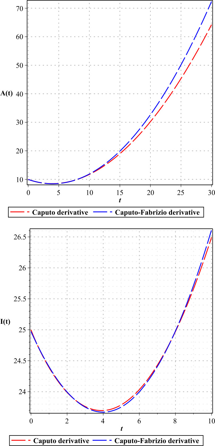
Plots of the results of Caputo derivative and Caputo–Fabrizio derivative for A, I with
Figure 1.
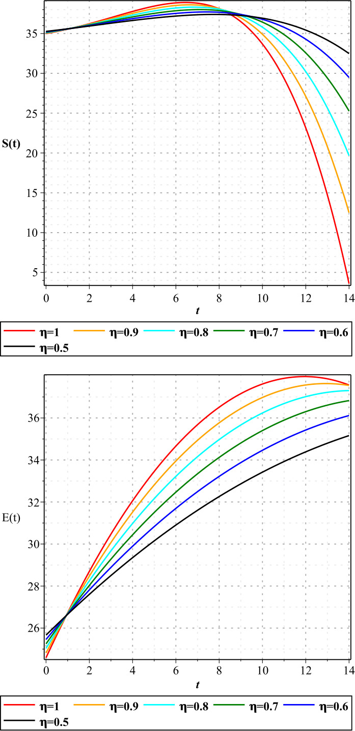
Plots of approximate solutions of susceptible parameter S and exposed parameter E for different values of
Figure 3.
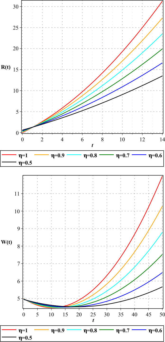
Plots of approximate solutions of removed parameter R and COVID-19 reservoir parameter W for different values of
Figure 2.
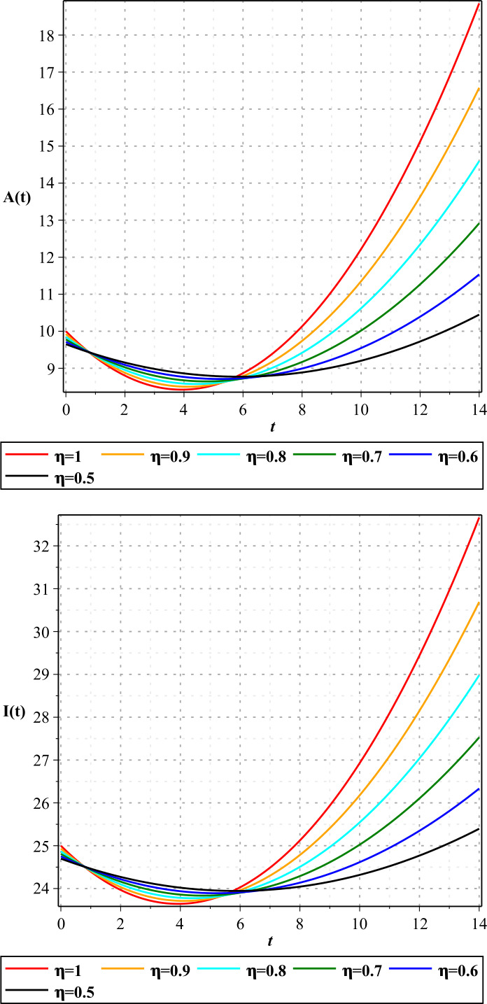
Plots of approximate solutions of asymptomatic infected parameter A and symptomatic infected parameter I for different values of
Figure 4.
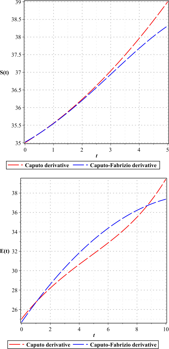
Plots of the results of Caputo derivative and Caputo–Fabrizio derivative for S, E with
Figure 6.
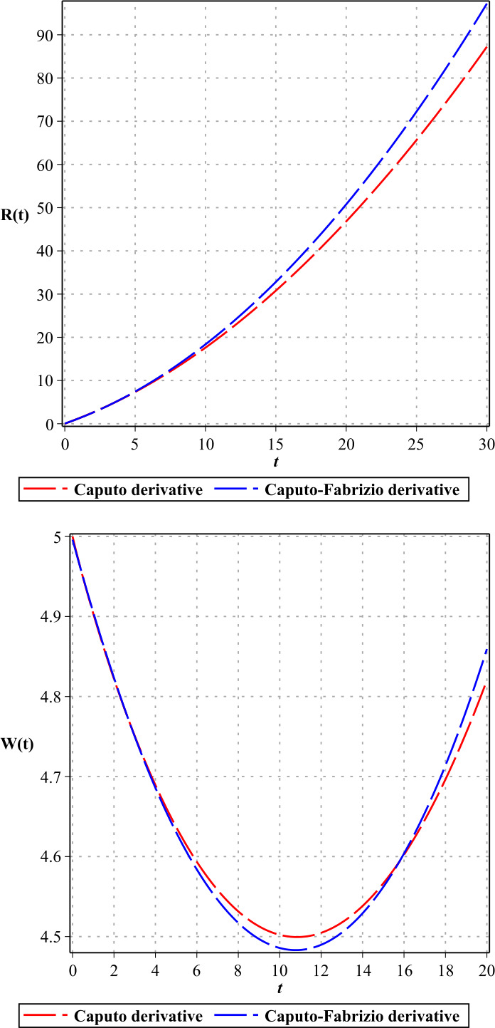
Plots of the results of Caputo derivative and Caputo–Fabrizio derivative for R, W with
Conclusion
In this paper, we investigate a model of the COVID-19 transmission in different groups of people using the Caputo–Fabrizio fractional derivative. Using the fixed point theorem, we prove a unique solution for the system. The resulting differential system is solved using the homotopy analysis transform method (HATM), and we obtain approximate solutions in convergent series. With the numerical results, we present a simulation for COVID-19, which shows the rapid transmission of the virus to different groups of people. We compared the results of the Caputo–Fabrizio fractional derivative with those of the Caputo derivative.
Acknowledgments
Acknowledgements
Research of the third author was supported by Azarbaijan Shahid Madani University. Also, research of the second author was supported by Miandoab Branch of Islamic Azad University. The authors are thankful to dear referees for the valuable comments which improved the final version of this work.
Availability of data and materials
Data sharing not applicable to this article as no datasets were generated or analyzed during the current study.
Authors’ contributions
The authors declare that the study was realized in collaboration with equal responsibility. All authors read and approved the final manuscript.
Funding
Not available.
Ethics approval and consent to participate
Not applicable.
Competing interests
The authors declare that they have no competing interests.
Consent for publication
Not applicable.
References
- 1.Haq F., Shah K., Rahman G., Shahzad M. Cancer treatment model with the Caputo–Fabrizio fractional derivative. Comput. Methods Differ. Equ. 2017;5(1):1–11. [Google Scholar]
- 2.Koca I. Analysis of rubella disease model with non-local and non-singular fractional derivatives. Int. J. Optim. Control Theor. Appl. 2018;8(1):17–25. [Google Scholar]
- 3.Rida S.Z., Arafa A.A.M., Gaber Y.A. Solution of the fractional epidemic model by L-ADM. J. Fract. Calc. Appl. 2016;7(1):189–195. [Google Scholar]
- 4.Singh H., Dhar J., Bhatti H.S., Chandok S. An epidemic model of childhood disease dynamics with maturation delay and latent period of infection. Model. Earth Syst. Environ. 2016;2:79. [Google Scholar]
- 5.Tchuenche J.M., Dube N., Bhunu C.P., Smith R.J., Bauch C.T. The impact of media coverage on the transmission dynamics of human influenza. BMC Public Health. 2011;11:S5. doi: 10.1186/1471-2458-11-S1-S5. [DOI] [PMC free article] [PubMed] [Google Scholar]
- 6.Upadhyay R.K., Roy P. Spread of a disease and its effect on population dynamics in an eco-epidemiological system. Commun. Nonlinear Sci. Numer. Simul. 2014;19(12):4170–4184. [Google Scholar]
- 7.Khan M.A., Atangana A. Modeling the dynamics of novel coronavirus (2019-ncov) with fractional derivative. Alex. Eng. J. 2020 [Google Scholar]
- 8.Babaei A., Jafari H., Ahmadi M. A fractional order HIV/AIDS model based on the effect of screening of unaware infectives. Math. Methods Appl. Sci. 2019;42(7):2334–2343. [Google Scholar]
- 9.Babaei A., Jafari H., Jalab H.A., Hadid S.B. Local fractional system for economic order quantity using entropy solution. Adv. Differ. Equ. 2019;2019:96. [Google Scholar]
- 10.Baleanu D., Mohammadi H., Rezapour S. A mathematical theoretical study of a particular system of Caputo–Fabrizio fractional differential equations for the rubella disease model. Adv. Differ. Equ. 2020;2020:184. doi: 10.1186/s13662-020-02762-2. [DOI] [PMC free article] [PubMed] [Google Scholar]
- 11.Akbari Kojabad E., Rezapour S. Approximate solutions of a sum-type fractional integro-differential equation by using Chebyshev and Legendre polynomials. Adv. Differ. Equ. 2017;2017:351. [Google Scholar]
- 12.Alizadeh S., Baleanu D., Rezapour S. Analyzing transient response of the parallel RCL circuit by using the Caputo–Fabrizio fractional derivative. Adv. Differ. Equ. 2020;2020:55. doi: 10.1186/s13662-020-02762-2. [DOI] [PMC free article] [PubMed] [Google Scholar]
- 13.Baleanu D., Agarwal R.P., Mohammadi H., Rezapour S. Some existence results for a nonlinear fractional differential equation on partially ordered Banach spaces. Bound. Value Probl. 2013;2013:112. [Google Scholar]
- 14.Baleanu D., Etemad S., Pourrazi S., Rezapour S. On the new fractional hybrid boundary value problems with three-point integral hybrid conditions. Adv. Differ. Equ. 2019;2019:473. [Google Scholar]
- 15.Baleanu D., Ghafarnezhad K., Rezapour S., Shabibi M. On the existence of solutions of a three steps crisis integro-differential equation. Adv. Differ. Equ. 2018;2018:135. [Google Scholar]
- 16.Baleanu D., Ghafarnezhad K., Rezapour S. On a three steps crisis integro-differential equation. Adv. Differ. Equ. 2019;2019:153. [Google Scholar]
- 17.Baleanu D., Hedayati V., Rezapour S., Al-Qurashi M.M. On two fractional differential inclusions. SpringerPlus. 2016;5(1):882. doi: 10.1186/s40064-016-2564-z. [DOI] [PMC free article] [PubMed] [Google Scholar]
- 18.Baleanu D., Jajarmi A., Mohammadi H., Rezapour S. A new study on the mathematical modeling of human liver with Caputo–Fabrizio fractional derivative. Chaos Solitons Fractals. 2020;134:109705. [Google Scholar]
- 19.Baleanu D., Mohammadi H., Rezapour S. On a nonlinear fractional differential equation on partially ordered metric spaces. Adv. Differ. Equ. 2013;2013:83. [Google Scholar]
- 20.Baleanu D., Rezapour S., Mohammadi H. Some existence results on nonlinear fractional differential equations. Philos. Trans. R. Soc. A. 2013;371:20120144. doi: 10.1098/rsta.2012.0144. [DOI] [PubMed] [Google Scholar]
- 21.Baleanu D., Mohammadi H., Rezapour S. The existence of solutions for a nonlinear mixed problem of singular fractional differential equations. Adv. Differ. Equ. 2013;2013:359. [Google Scholar]
- 22.Baleanu D., Mohammadi H., Rezapour S. Analysis of the model of HIV-1 infection of CD4+ T-cell with a new approach of fractional derivative. Adv. Differ. Equ. 2020;2020:71. [Google Scholar]
- 23.Baleanu D., Mousalou A., Rezapour S. On the existence of solutions for some infinite coefficient-symmetric Caputo–Fabrizio fractional integro-differential equations. Bound. Value Probl. 2017;2017:145. [Google Scholar]
- 24.Baleanu D., Rezapour S., Saberpour Z. On fractional integro-differential inclusions via the extended fractional Caputo–Fabrizio derivation. Bound. Value Probl. 2019;2019:79. [Google Scholar]
- 25.Talaee M., Shabibi M., Gilani A., Rezapour S. On the existence of solutions for a pointwise defined multi-singular integro-differential equation with integral boundary condition. Adv. Differ. Equ. 2020;2020:41. [Google Scholar]
- 26.Caputo M., Fabrizio M. A new definition of fractional derivative without singular kernel. Prog. Fract. Differ. Appl. 2015;1(2):73–85. [Google Scholar]
- 27.Aydogan S.M., Baleanu D., Mousalou A., Rezapour S. On approximate solutions for two higher-order Caputo–Fabrizio fractional integro-differential equations. Adv. Differ. Equ. 2017;2017(1):221. [Google Scholar]
- 28.Aydogan M.S., Baleanu D., Mousalou A., Rezapour S. On high order fractional integro-differential equations including the Caputo–Fabrizio derivative. Bound. Value Probl. 2018;2018(1):90. [Google Scholar]
- 29.Baleanu D., Mousalou A., Rezapour S. A new method for investigating approximate solutions of some fractional integro-differential equations involving the Caputo–Fabrizio derivative. Adv. Differ. Equ. 2017;2017:51. [Google Scholar]
- 30.Baleanu D., Mousalou A., Rezapour S. The extended fractional Caputo-Fabrizio derivative of order on and the existence of solutions for two higher-order series-type differential equations. Adv. Differ. Equ. 2018;2018:255. [Google Scholar]
- 31.Dokuyucu M.A., Celik E., Bulut H., Baskonus H.M. Cancer treatment model with the Caputo–Fabrizio fractional derivative. Eur. Phys. J. Plus. 2018;133:92. [Google Scholar]
- 32.Khan M.A., Hammouch Z., Baleanu D. Modeling the dynamics of hepatitis e via the Caputo–Fabrizio derivative. Math. Model. Nat. Phenom. 2019;14(3):311. [Google Scholar]
- 33.Ucar E., Ozdemir N., Altun E. Fractional order model of immune cells influenced by cancer cells. Math. Model. Nat. Phenom. 2019;14(3):308. [Google Scholar]
- 34.Ullah S., Khan M.A., Farooq M., Hammouch Z., Baleanu D. A fractional model for the dynamics of tuberculosis infection using Caputo–Fabrizio derivative. Discrete Contin. Dyn. Syst. 2020;13(3):975–993. [Google Scholar]
- 35.Dighe A., Jombart T., Kerkhove M.V., Ferguson N. A mathematical model of the transmission of middle east respiratory syndrome corona virus in dromedary camels (Camelus dromedarius) Int. J. Infect. Dis. 2019;79(S1):1–150. [Google Scholar]
- 36.Zhou Y., Ma Z., Brauer F. A discrete epidemic model for SARS transmission and control in China. Math. Comput. Model. 2004;40(13):1491–1506. doi: 10.1016/j.mcm.2005.01.007. [DOI] [PMC free article] [PubMed] [Google Scholar]
- 37.Chen T., Rui J., Wang Q., Zhao Z., Cui J.A., Yin L. A mathematical model for simulating the transmission of Wuhan novel coronavirus. Infect. Dis. Poverty. 2020;9:24. doi: 10.1186/s40249-020-00640-3. [DOI] [PMC free article] [PubMed] [Google Scholar]
- 38.Losada J., Nieto J.J. Properties of the new fractional derivative without singular kernel. Prog. Fract. Differ. Appl. 2015;1(2):87–92. [Google Scholar]
- 39.Belgacem F.B.M., Karaballi A.A., Kalla S.L. Analytical investigations of the Sumudu transform and applications to integral production equations. Math. Probl. Eng. 2003;3:103–118. [Google Scholar]
- 40.Bodkhe D.S., Panchal S.K. On Sumudu transform of fractional derivatives and its applications to fractional differential equations. Asian J. Math. Comput. Res. 2016;11(1):69–77. [Google Scholar]
- 41.Shah K., Junaid N.A.M. Extraction of Laplace, Sumudu, Fourier and Mellin transform from the natural transform. Appl. Environ. Biol. Sci. 2015;5(9):1–10. [Google Scholar]
- 42.Watugala G.K. Sumudu transform: a new integral transform to solve differential equations and control engineering problems. Int. J. Math. Educ. Sci. Technol. 1993;24(1):35–43. [Google Scholar]
- 43.Ullah M.Z., Alzahrani A.K., Baleanu D. An efficient numerical technique for a new fractional tuberculosis model with nonsingular derivative operator. J. Taibah Univ. Sci. 2019;13(1):1147–1157. [Google Scholar]
- 44.Wang J., Zhou Y., Medved M. Picard and weakly Picard operators technique for nonlinear differential equations in Banach spaces. J. Math. Anal. Appl. 2012;389(1):261–274. [Google Scholar]
- 45.Khuri S.A. A Laplace decomposition algorithm applied to a class of nonlinear differential equations. J. Appl. Math. 2001;1(4):141–155. [Google Scholar]
- 46.Liao S.J. Beyond Perturbation: Introduction to Homotopy Analysis Method. New York: Chapman & Hall/CRC Press; 2003. [Google Scholar]
Associated Data
This section collects any data citations, data availability statements, or supplementary materials included in this article.
Data Availability Statement
Data sharing not applicable to this article as no datasets were generated or analyzed during the current study.


