SEIR modeling of the COVID-19 and its dynamics

Abstract

In this paper, a SEIR epidemic model for the COVID-19 is built according to some general control strategies, such as hospital, quarantine and external input. Based on the data of Hubei province, the particle swarm optimization (PSO) algorithm is applied to estimate the parameters of the system. We found that the parameters of the proposed SEIR model are different for different scenarios. Then, the model is employed to show the evolution of the epidemic in Hubei province, which shows that it can be used to forecast COVID-19 epidemic situation. Moreover, by introducing the seasonality and stochastic infection the parameters, nonlinear dynamics including chaos are found in the system. Finally, we discussed the control strategies of the COVID-19 based on the structure and parameters of the proposed model.

Introduction

At the end of 2019, a novel coronavirus disease (COVID-19) was declared as a major health hazard by World Health Organization (WHO). At present, this disease is rapidly growing in many countries, and the global number of COVID-19 cases is increasing at a rapid rate. This coronavirus is a kind of enveloped, single stranded and positive sense virus which belongs to the RNA coronaviridae family [1, 2]. In early December of 2019, this infectious disease has begun to outbreak in Wuhan, the capital city of Hubei province, China. Until now, the epidemic in China is basically under control, but there are still many infections around the world. To defeat the epidemic, scientists in different fields investigated the COVID-19 from different points of view. Those aspects include pathology, sociology perspective, the infection mechanism and prediction [3–8].

In the history of mankind, there are many other outbreak and transmission of diseases such as dengue fever, malaria, influenza, pestilence and HIV/AIDS. How to built a proper epidemiological model for these epidemics is a challenging task. Some scientists treat the disease spread as a complex network for forecast and modeling [9, 10]. For the COVID-19, Bastian Prasse et al. [10] designed a network-based model which is built by the cities and traffic flow to describe the epidemic in the Hubei province. At present, the SIS [11, 12], SIR[13] and SEIR [14, 15] models provide another way for the simulation of epidemics. Lots of research works have been reported. It shows that those SIS, SIR and SEIR models can reflect the dynamics of different epidemics well. Meanwhile, these models have been used to model the COVID-19 [16, 17]. For instance, Tang et al. [17] investigated a general SEIR-type epidemiological model where quarantine, isolation and treatment are considered. Moreover, there are also other methods for modeling of the COVID-19 [18, 19]. Wang et al. [19] applied the phase-adjusted estimation for the number of coronavirus disease 2019 cases in Wuhan. Thus in this paper, we try to propose a SEIR model to simulate the process of COVID-19.

Chaos widely exits in nature and man-made systems including those biological systems [20–24]. According to the famous Logistic map, it shows that the natural evolution of the population size could be chaotic. However, it is not a good thing to find chaos in the SEIR model. Unfortunately, chaos in the SIR, SIS and SEIR models has been investigated by many researchers. Generally, the seasonality and stochastic infection are introduced to the system for the nonlinear dynamics. For instance, Kuznetsov and Piccardi [25] investigated the bifurcations of the periodic solutions of SEIR and SIR epidemic models with sinusoidally varying contact rate. Meanwhile, the fractional-order SEIR epidemic model has aroused research interests of scientists. He et al. [26] investigated the epidemic outbreaks using the SIR model, and a hard limited controller is designed for the control of the system. However, on the one hand, those SIR and SEIR models cannot always show the nature of the COVID-19, and we need to modify the system. On the other hand, the nonlinear dynamics of the system should be investigated. Thus, we need to get more information on the dynamics of the epidemic system.

The rest of this paper is organized as follows. In Sect. 2, the modified SEIR model is designed and the descriptions of the system are presented. In Sect. 3, the SEIR model is applied to the COVID-19 data of Hubei province where the PSO algorithm is introduced to estimate the parameters. In Sect. 4, the seasonality and stochastic infection are introduced to the model and the dynamics of the system is investigated. In Sect. 5, the structure, parameters on the dynamics of the system and how to control the epidemic of the system are discussed. Section 6 is the summary of the analysis.

SEIR modeling of the COVID-19

The classical SEIR model has four elements which are S (susceptible), E (exposed), I (infectious) and R (recovered). Thus, $N=S+E+I+R$ means the total number of people. The basic hypothesis of the SEIR model is that all the individuals in the model will have the four roles as time goes on. The SEIR model has some limitations for the real situations, but it provides a basic model for the research of different kinds of epidemic.

Based on the basic SEIR model, we proposed a new model which is denoted by

$$\begin{array}{c}\hfill \left\{\begin{array}{c}\dot{S}=-\frac{S}{N}\left({\beta }_1{I}_1+{\beta }_2{I}_2+\chi E\right)+{\rho }_{1}Q-{\rho }_{2}S+\alpha R\hfill \\ \dot{E}=\frac{S}{N}\left({\beta }_1{I}_1+{\beta }_2{I}_2+\chi E\right)-{\theta }_{1}E-{\theta }_{2}E\hfill \\ {\dot{I}}_1={\theta }_{1}E-{\gamma }_1{I}_1\hfill \\ {\dot{I}}_2={\theta }_{2}E-{\gamma }_2{I}_2-\phi I_2+\lambda \left(\Lambda ,+,Q\right)\hfill \\ \dot{R}={\gamma }_1{I}_1+{\gamma }_2{I}_2+\varphi H-\alpha R\hfill \\ \dot{H}=\phi I_2-\varphi H\hfill \\ \dot{Q}=\Lambda +{\rho }_{2}S-\lambda \left(\Lambda +Q\right)-{\rho }_{1}Q\hfill \end{array}\right),\end{array}$$ 1

where S, E, $I_1$, $I_2$, R, H and Q are the system variables. The descriptions of those variables are presented in Table 1. The description of the system parameters is illustrated in Table 2, and the relationship between different variables is shown in Fig. 1. In this model, the infectious class is divided into two parts, $I_1$ and $I_2$. Meanwhile, we consider the quarantined class and hospitalized class in the model according to the real situation. For example, if one got coronavirus-like symptoms or comes from other place like abroad, he or she needs to be in quarantine for at least 14 days.

Table 1.

Description of the system variables

Variable	Description
S	Susceptible class
E	Exposed
$I_1$	Infectious without intervention
$I_2$	Infectious with intervention
R	Recovered
Q	Quarantined
H	Hospitalized

Table 2.

Description of the system parameters

Parameters	Description
$\alpha$	Temporary immunity rate
${\beta }_1$, ${\beta }_2$	The contact and infection rate of transmission per contact from infected class
$\chi$	Probability of transmission per contact from exposed individuals
${\theta }_1$, ${\theta }_2$	Transition rate of exposed individuals to the infected class
${\gamma }_1$, ${\gamma }_2$	Recovery rate of symptomatic infected individuals to recovered
$\phi$	Rate of infectious with symptoms to hospitalized
$\varphi$	Recovered rate of quarantined infected individuals
$\lambda$	Rate of the quarantined class to the recovered class
${\rho }_1$, ${\rho }_2$	Transition rate of quarantined exposed between the quarantined infected class and the wider community
$\Lambda$	External input from the foreign countries

Fig. 1.

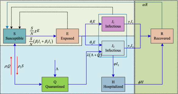
Flowchart of the proposed SEIR model for COVID-19

Obviously, as shown in Fig. 1, we consider two main channels in the proposed model. The first one goes to $S\to E\to I_1\to R$, and the second channel goes to $S\to Q\to I_2\to H\to R$. The first case shows the natural process of the epidemic, and it is a typical SEIR model. The second channel considers the control from the government including the quarantine and hospital. As a result, the designed model is an improved version of the SEIR model.

If there is no quarantine (${\rho }_2=0$), hospital treatment $\varphi =0$ and the recovered is immune to the virus ($\alpha =0$), the model becomes to the classical SEIR model. However, there are always quarantine and hospital treatment. Meanwhile, there is no evidence that the recovered is immune to the COVID-19. Thus, we need to considered these factors in the model. In this paper, we have $N\ne S+E+I_1+I_2+R+Q+H$ according to Eq. (1) since there is an external input $\Lambda$. Obviously, N is not a constant and it varies over time when $\Lambda \ne 0$. Since there are a large population under voluntary home quarantine. Thus, for a chosen place, N is not the total population of that place, but it can be estimated by adding the final number of recoveries and deaths.

Estimation of the model parameters

The PSO algorithm

Particle swarm optimization (PSO) algorithm is a famous population-based stochastic optimization algorithm motivated by intelligent collective behavior, such as the foraging process of bird group [27]. In PSO algorithm, each particle represents a bird, and the algorithm starts with a random initialization of the particle locations. For one iteration, each particle keeps track of its own best position and the population’s best position to update its position and velocity. Considering a one-dimensional optimization problem, the velocity and the position of the particle i is defined by

$$\begin{array}{c}\hfill \begin{array}{c}{V}_i(t+1)=\omega (t)V_i(t)+c_1{r}_1[P_{b,i}(t)-X_i(t)]\hfill \\ +c_2{r}_2[P_g(t)-X_i(t)]\hfill \end{array},\end{array}$$ 2

and

$$\begin{array}{c}\hfill X_i(t+1)=X_i(t)+V_i(t+1),\end{array}$$ 3

where $V_i(t)$ and $X_i(t)$ are velocity and position of the particle i at the t-th iteration, respectively. $c_1$ and $c_2$ are the learning factors. $r_1$ and $r_2$ are random numbers between 0 and 1. $P_{b,i}(t)$ represents the best position of the particle i at the t-th iteration, and $P_g(t)$ represents the population’s best position at the t-th iteration. $\omega$ is called inertia weight, which is very important for the search process of PSO algorithm. Here, it is defined by [28]

$$\begin{array}{c}\hfill \omega (t)=({\omega }_{\max }-{\omega }_{\min })e^{-500{(t/T)}^2}+{\omega }_{\min },\end{array}$$ 4

where t and T are the current and maximum iterations of the PSO algorithm, respectively, and ${\omega }_{\mathit{min}}$ and ${\omega }_{\mathit{max}}$ are the minimal and maximum value of the inertia weight, respectively. Suppose that we meet a minimum optimization problem, the implementation steps of the PSO algorithm are summarized as follows:

• Step 1: The position of each particle is randomly initialized.

• Step 2: Calculate the fitness value $F(X_i(t))$ of the particle i, and find the $P_{b,i}(t)$ and the $P_g(t)$.

• Step 3: If $F(X_i(t))<F(P_{b,i}(t))$, then replace the $P_{b,i}(t)$ by the $X_i(t)$.

• Step 4: If $F(X_i(t))<F(P_g(t))$, then replace the $P_g(t)$ by the $X_i(t)$.

• Step 5: Calculate the inertia weight by Eq. (4).

• Step 6: Update velocity and position of the particle i according to Eqs. (2) and (3), respectively.

• Step 7: Repeat the Steps 3–6 until the termination criterion is satisfied.

Parameter estimation

In this section, through the actual COVID-19 data from Hubei province, the PSO algorithm is utilized to estimate the parameters of the proposed SEIR model to fit the real situation. The COVID-19 data come from the official website of the Wuhan Municipal Health Commission (http://wjw.wh.gov.cn/), and some actual data are listed in Table 3.

Table 3.

Actual COVID-19 data from Hubei (January 24th to February 8th)

Date	Cumulative infected cases	Cumulative deaths	Cumulative recovered cases	Current quarantined
2020/1/24	729	39	32	4711
2020/1/25	1052	52	42	6904
2020/1/26	1423	76	44	9103
2020/1/27	2714	100	47	15,559
2020/1/28	3554	125	80	20,366
2020/1/29	4586	162	90	26,632
2020/1/30	5806	204	116	32,340
2020/1/31	7153	249	166	36,838
2020/2/1	9074	294	215	43,121
2020/2/2	11,177	350	295	48,171
2020/2/3	13,522	414	396	58,544
2020/2/4	16,678	479	520	66,764
2020/2/5	19,665	549	633	64,127
2020/2/6	22,112	618	817	64,057
2020/2/7	24,953	699	1115	67,802
2020/2/8	27,100	780	1439	70,438
......

In the face of the pressure of epidemic prevention and control, Wuhan government announced to seal off the city from all outside contact on January 23rd, 2020. Then, other cities in Hubei province also took the “closure city” measure. The COVID-19 epidemic situation of Hubei is relatively stable after January 23rd, 2020, so we chose to study the data between January 24th and April 12th.

The initial values setting of SEIR model is presented in Table 4, where N is the total population of Hubei affected by the COVID-19 epidemic in January 24th, 2020, and E is calculated based on the number of confirmed patients. $I_1$ is an estimated value based on $I_2$, and the other initial values are originated from the actual data.

Table 4.

Initial values of the SEIR model

Parameter	N	E	$I_1$	$I_2$	H	R	Q	$\Lambda$
Value	$6.5563\times {10}^4$	5077	$I_2\times 0.01$	729	658	32	4711	10

The system parameters of SEIR model are calculated by the actual data, as shown in Table 5. However, there is no accurate statistics of the rate of infectious to hospitalized $\phi$ and the recovered rate of quarantined infected individuals $\varphi$. Here, the two parameters are estimated by the PSO algorithm with the actual data of R and H. The settings of PSO algorithm are set as: population of particle swarm $NP=40$, learning factors $c_1=c_2=2$, maximal iteration $T=100$ and the search spaces $\phi ,\varphi \in (0,0.1]$.

Table 5.

System parameters of SEIR model

Parameter	Values
${\beta }_1$	$1.0538\times {10}^{-1}$
${\beta }_2$	$1.0538\times {10}^{-1}$
$\chi$	$1.6221\times {10}^{-1}$
${\rho }_1$	$2.8133\times {10}^{-3}$
${\rho }_2$	$1.2668\times {10}^{-1}$
${\theta }_1$	$9.5000\times {10}^{-4}$
${\theta }_2$	$3.5412\times {10}^{-2}$
${\gamma }_1$	$8.5000\times {10}^{-3}$
${\gamma }_2$	$1.0037\times {10}^{-3}$
$\lambda$	$9.4522\times {10}^{-2}$
$\alpha$	$1.2048\times {10}^{-4}$

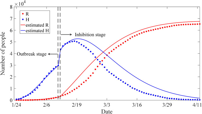
The COVID-19 epidemic situation in Hubei is divided into two stages: the outbreak stage (the first 19 days) and the inhibition stage (the 20th day to the end).

In the outbreak stage, according to the actual data of R and H, the $\phi$ and the $\varphi$ are estimated to $\phi =0.2910$, $\varphi =0.0107$, respectively. The error convergence curve of PSO is shown in Fig. 2. After the outbreak stage, due to the continuous assistance from other provinces and other countries, the epidemic in Hubei began to enter the inhibition stage. In this stage, the error convergence curve of PSO is given in Fig. 3, and the estimated $\phi$ and $\varphi$ changed to $\phi =0.0973,\varphi =0.0416$, respectively.

Fig. 2.

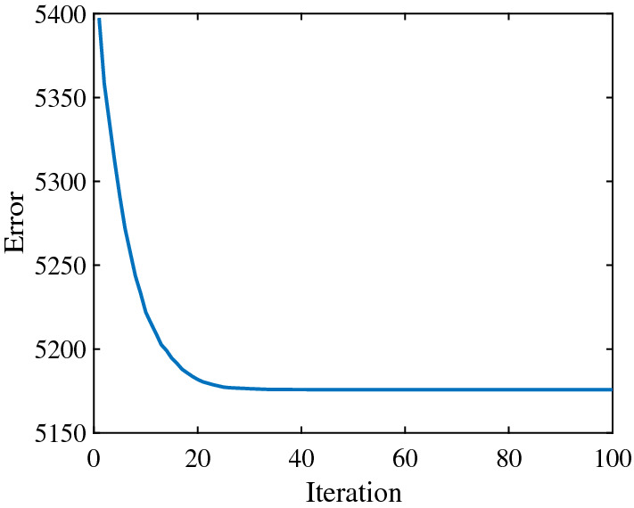
The error convergence curve of PSO algorithm in the outbreak stage

Fig. 3.

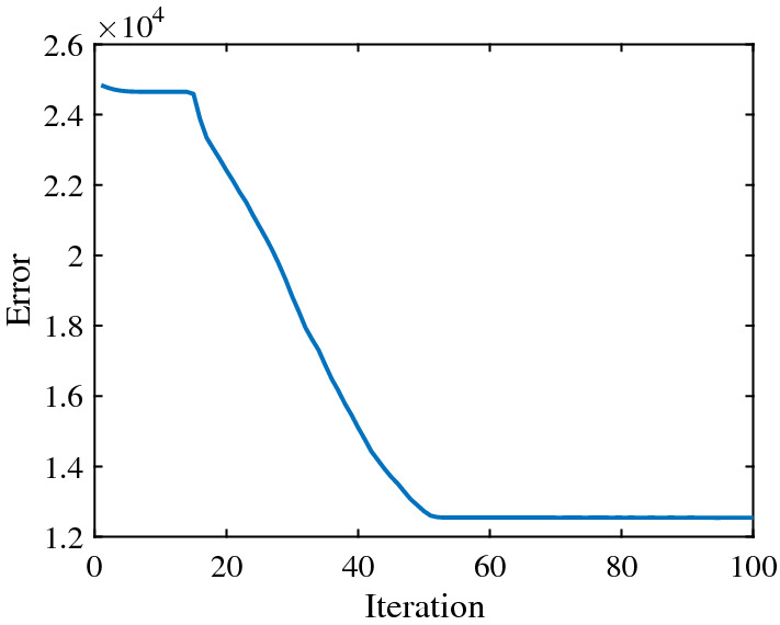
The error convergence curve of PSO algorithm in the inhibition stage

The estimated and actual trajectories in the two stages are shown in Fig. 4. In the first stage, although there are some errors between the estimated number and the actual number, it shows that the estimated values match well with the real situation. However, the accuracy is not satisfying in the second stage which shows that the real data are smaller than the estimated values, but the trend is basically the same.

Fig. 4.

Actual and estimated trajectories for the epidemic situation in Hubei province

There are two reasons for the deviation. One is that only two parameters, namely the rate of infectious to hospitalized $\phi$ and the recovered rate of quarantined infected individuals $\varphi$, are estimated, while the rest of the parameters are set as a matter of experience. Moreover, the control measures for containing the outbreak are more and more powerful; thus, the system parameter should be time varying variables. For instance, compared with the outbreak stage, the hospitalization rate decreased a lot, and the cure rate increased nearly four times, which means that the number of confirmed infected cases is declining a lot and the number of patients recovering is increasing rapidly.

Nonlinear dynamics of the model

SEIR model with seasonality and stochastic infection

The 0–1 test algorithm is employed to verify the existence of chaos in the model. If a set of discrete time series $x(n)(n=1,2,3,\dots )$ represents a one-dimensional observable data set obtained from the modified SEIR system, then the following two real-valued sequences are defined as [30]

$$\begin{array}{c}\hfill \left\{\begin{array}{c}p\left(n\right)={\sum }_{j=1}^{n}x\left(j\right)cos\left(\theta \left(j\right)\right)\hfill \\ s\left(n\right)={\sum }_{j=1}^{n}x\left(j\right)sin\left(\theta \left(j\right)\right)\hfill \end{array}\right),\end{array}$$ 5

where $\theta \left(j\right)=j\eta +\sum _{i=1}^{j}x\left(i\right)$, and $\eta \in \left[\frac{\pi }{5},\frac{4\pi }{5}\right]$. By plotting the trajectories in the (p, s)-plane, the state of the system can be identified. Usually, the bounded trajectories in the (p, s)-plane imply the dynamics of the time series is regular, while Brownian-like (unbounded) trajectories imply chaos.

The seasonality is widely found in the epidemic models [26, 29], and it can make the system more complex. Indeed, there is no report showing that the effect of seasonality for COVID-19 spread since this epidemic outbreaks only about half year until now. But we try to introduce the seasonality to the system and analyze chaos in the system from an academic point of view. Meanwhile, there are individual differences and many unpredictable factors in the epidemic infection. Thus, the noise is an important factor considered in our analysis. Here, three cases are analyzed to show how the system parameter $\alpha$, seasonality and stochastic infection affect the dynamics of the system.

Case 1: The parameter ${\beta }_1$ contains seasonality and stochastic infection, and the three contact and infection rate parameters are defined as

$$\begin{array}{c}\hfill \left\{\begin{array}{c}{\beta }_2=30.03,\chi =30.40\hfill \\ {\beta }_1\left(t\right)={\beta }_0\left(1+{\epsilon }_{1}sin\left(2\pi t\right)+{\epsilon }_2\xi \left(t\right)\right)\hfill \end{array}\right),\end{array}$$ 6

where ${\beta }_0=2\times {\beta }_1=60$, ${\epsilon }_1$ and ${\epsilon }_2$ are degree of the seasonality and stochastic infection, respectively. $〈\xi ,\left(t\right)〉$ is the white Gaussian independent noises, and it has the properties of $〈\xi ,\left(t\right)〉=0$ and $〈\xi \left(t\right),\xi \left(\tau \right)〉=\delta \left(t-\tau \right)$.

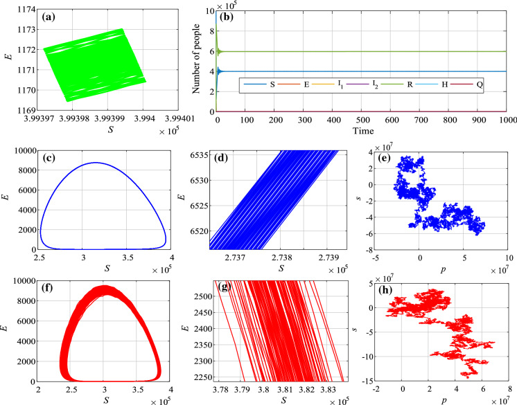
The analysis results of the system with different parameters are shown in Fig. 5. In Fig. 5a, b, we set ${\epsilon }_1=0$, ${\epsilon }_2=0$ and $\alpha =0.08$. It shows that the system is convergent to a limited region. Thus, the system is not chaotic without the seasonality and stochastic infection. When ${\epsilon }_1=0.8$ and ${\epsilon }_2=0$, the system has seasonality but no stochastic infection. It shows that the system now is chaotic according to the $p-s$ plot. As shown in Fig. 5c that the attractor looks like a limited circle. However, there are many lines in the “circle” as it is illustrated in Fig. 5d. If ${\epsilon }_1=0.8$ and ${\epsilon }_2=0.2$, there are both seasonality and stochastic infection in the system. At this time, the complex dynamics is observed in the system, as shown in Fig. 5f–h.

Fig. 5.

Dynamics analysis results of case 1 with different parameters. Phase diagram a and time series b of the system with ${\epsilon }_1=0$, ${\epsilon }_2=0$ and $\alpha =0.08$; phase diagram c, its partial enlarged drawing d and $p-s$ plot e with ${\epsilon }_1=0.8$, ${\epsilon }_2=0$ and $\alpha =0.08$; phase diagram f, its partial enlarged drawing g and $p-s$ plot h with ${\epsilon }_1=0.8$, ${\epsilon }_2=0.2$ and $\alpha =0.08$

Case 2: The parameter ${\beta }_2$ contains seasonality and stochastic infection, while the other two infection rate parameters are constants. Thus, the parameters are defined as

$$\begin{array}{c}\hfill \left\{\begin{array}{c}{\beta }_1=30,\chi =30.40\hfill \\ {\beta }_2\left(t\right)={\beta }_0\left(1+{\epsilon }_{1}sin\left(2\pi t\right)+{\epsilon }_2\xi \left(t\right)\right)\hfill \end{array}\right),\end{array}$$ 7

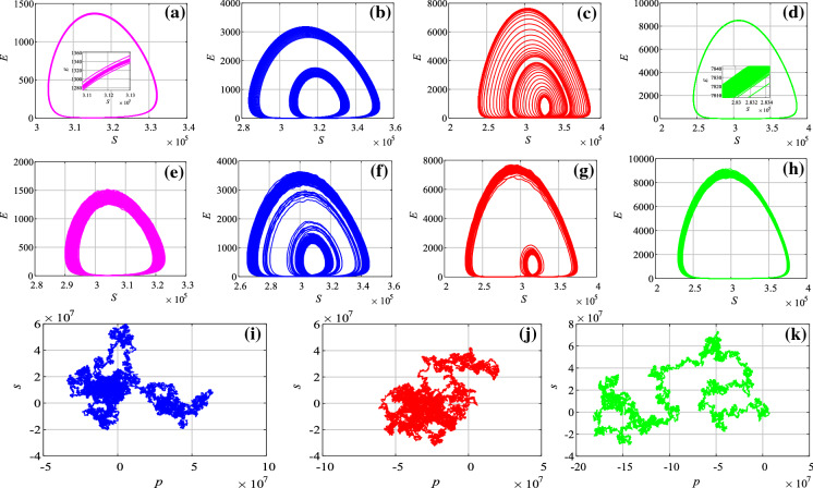
where ${\beta }_0=2\times {\beta }_2=60$, ${\epsilon }_1$ and ${\epsilon }_2$ are the degree of the seasonality and stochastic infection, respectively. Firstly, we let ${\epsilon }_1=0.8$ and ${\epsilon }_2=0$. If $\alpha =0.02$, $\alpha =0.03$, $\alpha =0.04747$ and $\alpha =0.08$, different kinds of chaotic attractors are shown in Fig. 6a–d, respectively. Meanwhile, we let ${\epsilon }_1=0.8$ and ${\epsilon }_2=0.2$, the chaotic attractors with different values of $\alpha$ are shown in Fig. 6e–h. The $p-s$ plots of attractors of Fig. 6b–d are shown in Fig. 6i–k, respectively. It verifies the existence of chaos in the model.

Fig. 6.

Dynamics analysis results of case 2. Phase diagrams with ${\epsilon }_1=0.8$, ${\epsilon }_2=0$ and $\alpha =0.02$ a, $\alpha =0.03$ b, $\alpha =0.04747$ c and $\alpha =0.08$ d; phase diagrams with ${\epsilon }_1=0.8$, ${\epsilon }_2=0.2$ and $\alpha =0.02$ e, $\alpha =0.03$ f, $\alpha =0.04747$ g and $\alpha =0.08$ h; $p-s$ plots of ${\epsilon }_1=0.8$, ${\epsilon }_2=0$ and $\alpha =0.03$ i, $\alpha =0.04747$ j and $\alpha =0.08$ k

Case 3: The parameter ${\chi }_1$ contains seasonality and stochastic infection, and ${\beta }_1$ and ${\beta }_2$ are contacts. As a results, the parameters in this case are given by

$$\begin{array}{c}\hfill \left\{\begin{array}{c}{\beta }_1=30,{\beta }_2\left(t\right)=30\hfill \\ \chi ={\chi }_0\left(1+{\epsilon }_{1}sin\left(2\pi t\right)+{\epsilon }_2\xi \left(t\right)\right)\hfill \end{array}\right)\end{array}$$ 8

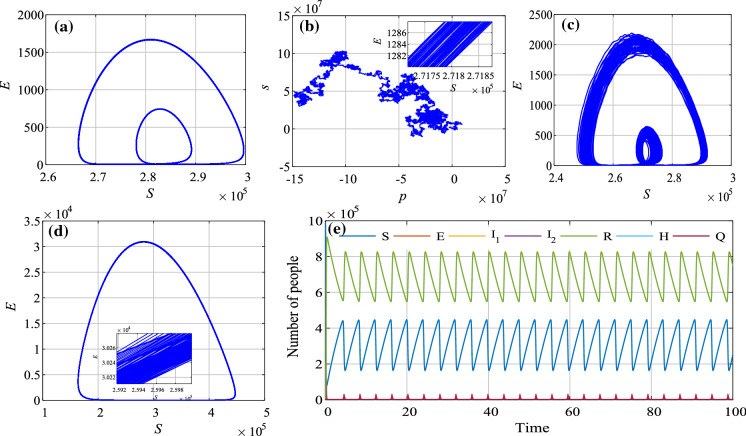
where ${\beta }_0=2\chi =60.8$, ${\epsilon }_1$ and ${\epsilon }_2$ are the degree of the seasonality and stochastic infection, respectively. Let ${\epsilon }_1=0.8$, ${\epsilon }_2=0$ and $\alpha =0.0133$, the phase diagram is shown in Fig. 7a. It shows in Fig. 7b that the attractor is chaotic. If we set ${\epsilon }_2=0.2$, the phase diagram is illustrated in Fig. 7c, where a much wider range in the phase space when the system has stochastic infection. When ${\epsilon }_1=0.8$, ${\epsilon }_2=0$ and $\alpha =0.08$, the phase diagram is shown in Fig. 7d, while the time series are shown in Fig. 7e.

Fig. 7.

Dynamics analysis results of case 3. Phase diagram a and $p-s$ plot b with ${\epsilon }_1=0.8$, ${\epsilon }_2=0$ and $\alpha =0.0133$; phase diagram c with ${\epsilon }_1=0.8$, ${\epsilon }_2=0.2$ and $\alpha =0.0133$; phase diagram d and time series e with ${\epsilon }_1=0.8$, ${\epsilon }_2=0.2$ and $\alpha =0.08$

The proposed system is an improved SEIR system with quarantined class and hospitalized class. As with other SIR and SEIR models, this model can also generate chaos with given parameters. And the existence chaos is verified by the 0–1 test method.

In this section, we consider the dynamics of the proposed SEIR model. In Refs. [26, 29], the parameters of the SEIR model are set where the infection rate $\beta$ is set as quite large values. For instance, in Ref. [29], $\beta =108$ for the proposed SEIR Dengue fever model. To investigate chaos in the proposed model, the parameters are set as ${\beta }_1=30$, ${\beta }_2=30.0300$, $\chi =30.40$, ${\rho }_1=1/14$, ${\rho }_2=0.002$, ${\theta }_1=20.054$, ${\theta }_2=20.12$, $\phi =0.00009$, $\varphi =0.8$, $\lambda =0.4$ and $N={10}^6$. The initial conditions of the model are given by $[S,E,I_1,I_2,R,H,Q]=[94,076,4007,262,524,31,100,1000]$.

Bifurcation analysis of case 2

To further analyze dynamics of the system, we choose case 2 as an example to show the bifurcations of the proposed system. The parameters are set as ${\beta }_1=30$, ${\beta }_2=30.0300$, $\chi =30.40$, ${\rho }_1=1/14$, ${\rho }_2=0.002$, ${\theta }_1=20.054$, ${\theta }_2=20.12$, $\phi =0.00009$, $\varphi =0.8$, $\lambda =0.4$ and $N={10}^6$. The initial conditions of the model are given by $[S,E,I_1,I_2,R,H,Q]$=[94076, 4007, 262, 524,31, 100, 1000].

Firstly, let ${\epsilon }_1=0.8$, ${\epsilon }_2=0$, and the parameter $\alpha$ varies from 0.02 to 0.08 with step size of 0.00024. The bifurcation diagram is shown in Fig. 8a. Meanwhile, if ${\epsilon }_2=0.2$, the corresponding bifurcation diagram is shown in Fig. 8b. Obviously, the bifurcation diagram of Fig. 8a has no noise, while that in Fig. 8b does. It shows that the stochastic infection makes the system fluctuate more volatile.

Fig. 8.

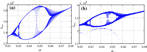
Bifurcation diagrams of the system with the variation of parameter $\alpha$ a ${\epsilon }_1=0.8$, ${\epsilon }_2=0$; b ${\epsilon }_1=0.8$, ${\epsilon }_2=0.2$

Secondly, let $\alpha =0.08$, ${\epsilon }_2=0$, and the parameter ${\epsilon }_1=0.8$ varies from 0.02 to 0.08 with step size of 0.004. The bifurcation diagrams with ${\epsilon }_1$ are shown in Fig. 9. It shows that when there exists stochastic infection, the bifurcation diagram shows more complex behaviors of the system.

Fig. 9.

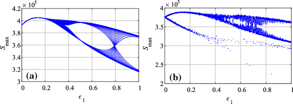
Bifurcation diagrams of the system with the variation of parameter ${\epsilon }_1$ a $\alpha =0.08$, ${\epsilon }_2=0$; b $\alpha =0.8$, ${\epsilon }_2=0.2$

As shown in Figs. 8 and 9, it shows that the system has rich dynamics with both parameters $\alpha$ and ${\epsilon }_1$. When the system has stochastic infection, the system will become more complex. We hold the opinion that chaos is also the nature of the system, and the seasonality and the temporary immunity rate can change the dynamics of the system.

Complexity of the case 2

In this section, the spectral entropy (SE) algorithm [31] is employed to analyze complexity of the proposed SEIR system, and steps are presented as follows.

For a given time series {x(n), n=0, 1, 2, $\cdots$, L-1} with a length of L, let $x(n)=x(n)-\overline{x}$, where $\overline{x}$ is the mean value of time series. Its corresponding discrete Fourier transform (DFT) is defined by

$$\begin{array}{c}\hfill X(k)=\sum _{n=0}^{L-1}x(n)e^{-j2\pi nk/L},\end{array}$$ 9

where $k=0,1,\cdots ,L-1$ and j is the imaginary unit. If the power of a discrete power spectrum with the $k_{\mathit{th}}$ frequency is ${|X(k)|}^2$, then the “probability” of this frequency is defined as

$$\begin{array}{c}\hfill P_k=\frac{{|X(k)|}^2}{{\sum }_{k=0}^{L/2-1}{|X(k)|}^2}.\end{array}$$ 10

When the DFT is employed, the summation runs from $k=0$ to $k=N/2-1$. The normalization entropy is denoted by [31]

$$\begin{array}{c}\hfill SE\left(x^L\right)=\frac{1}{ln\left(N/2\right)}\sum _{k=0}^{N/2-1}{P}_{k}ln\left(P_k\right),\end{array}$$ 11

where $\ln (N/2)$ is the entropy of a completely random signal. Obviously, the more balanced the probability distribution is, the higher complexity (the larger entropy) the time series is. The larger measuring value means higher complexity, and vice versa.

Based on the above complexity algorithms, multiscale complexity algorithm is designed. For a one-dimensional discrete time series $\{x(n):n=0,1,\dots ,N-1\}$, the consecutive coarse-grained time series are constructed by [32]

$$\begin{array}{c}\hfill y^{\tau }(j)=\frac{1}{\tau }\sum _{(j-1)\tau }^{j\tau -1}x(j),\end{array}$$ 12

where $1\le j\le [N/\tau ]$, $\tau$ is the scale factor which represents the length of the non-overlapping window, and $[·]$ denotes the floor function. Obviously, when $\tau =1$, the sequence $y^{\tau }$ is the original sequence $\{x(n),n=0,2,3,\cdots ,L-1\}$. Thus, the complexity of $y^1$ is the complexity of the original sequence. In this paper, the multiscale complexity is defined as [31]

$$\begin{array}{c}\hfill \mathrm{MSE}=\frac{1}{{\tau }_{max}}\sum _{\tau =1}^{{\tau }_{max}}\mathrm{SE}(y^{\tau }).\end{array}$$ 13

In this paper, we set ${\tau }_{\mathit{max}}=20$.

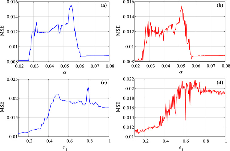
Fix ${\epsilon }_1=0.8$ and vary the parameter $\alpha$ from 0.02 to 0.08 with step size of 0.00024. MSE complexity analysis results are shown in Fig. 10a, b, where Fig. 10a for ${\epsilon }_2=0$ and Fig. 10b for ${\epsilon }_2=0.2$. Fix $\alpha =0.08$ and the parameter ${\epsilon }_1$ varies from 0.1 to 1 with step size of 0.0036. The complexity analysis results with ${\epsilon }_1$ are shown in Fig. 10c, d. Here, ${\epsilon }_2=0$ is employed in Fig. 10c, while ${\epsilon }_2=0.2$ is used in Fig. 10d. The complexity analysis results with parameters show that the stochastic infection does not affect the complexity of the system. The system has higher complexity when $\alpha$ takes values between 0.03 and 0.06, and ${\epsilon }_1$ takes those values which are larger than 0.6.

Fig. 10.

MSE analysis results of the system with the variation of parameters $\alpha$ and ${\epsilon }_1$ a ${\epsilon }_1=0.8$, ${\epsilon }_2=0$ and $\alpha$ varying; b ${\epsilon }_1=0.8$, ${\epsilon }_2=0.2$ and $\alpha$ varying; c $\alpha =0.08$, ${\epsilon }_2=0$ and ${\epsilon }_1$ varying; d $\alpha =0.08$, ${\epsilon }_2=0.2$ and ${\epsilon }_1$ varying

Fix ${\epsilon }_2=0$, vary $\alpha$ from 0.02 to 0.08 with step size of 0.0006 and ${\epsilon }_1$ varies from 0.1 to 1 with step size of 0.009. The complexity analysis result in the $\alpha -{\epsilon }_1$ plane is shown in Fig. 11. Obviously, the higher complexity region is located in the right side of the parameter plane, where $\alpha \in [0.4,1]$ and ${\epsilon }_1\in [0.025,0.055]$.

Fig. 11.

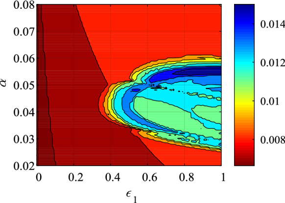
MSE analysis results of the system with the variation of both parameters $\alpha$ and ${\epsilon }_1$

Since the complexity measure results are obtained based on the generated time series, MSE provides an effective way for the dynamics analysis of the system. When there is higher complexity, the behavior of the model is more complex, vice versa. For a epidemic system, high complexity means outbreak. Thus, we can use the complexity measure algorithm to monitor the dynamics of the proposed SEIR system.

Discussion

In this paper, the parameters of the system are mainly chosen by two means including the references and the PSO algorithm. Usually, the parameters can be set according to the existing work. For instance, the contact and infection rate parameters are defined according to Refs. [26, 29]. Also, there are some other references which show some parameters of the system. Moreover, since there is actual COVID-19 data from Hubei province, we use the PSO algorithm to estimate the parameters of the system. As shown above, the system has rich dynamics with the given parameters, especially when the parameters ${\beta }_1$, ${\beta }_2$ and $\chi$ have seasonality and stochastic infection. The existence of chaos is verified by the 0–1 test, and complexity of the generated time series is measured. Here, different sets of parameters are summarized in Table 6. It should noted that, when the parameters are set as the set A, they seem “large.” However, those parameters should be multiplied by S/N. Thus, they are reasonable for the proposed model. According to our analysis, it shows that chaos are found in the system with those “large parameters.” In fact, we want to explore the nonlinear dynamics of the proposed system and to study how does chaos occur in the system.

Table 6.

Values of the parameters for different cases

Parameters	Set A (Chaos)	Set B (Stage 1)	Set C (Stage 2)	Set D (Test)
$\alpha$	0.08	$1.2048\times {10}^{-4}$	$1.2048\times {10}^{-4}$	0 or 0.5
${\beta }_1$,	30	$1.0538\times {10}^{-1}$	$1.0538\times {10}^{-1}$	0.01
${\beta }_2$	30.03	$1.0538\times {10}^{-1}$	$1.0538\times {10}^{-1}$	0.3
$\chi$	30.40	$1.6221\times {10}^{-1}$	$1.6221\times {10}^{-1}$	0.4
${\theta }_1$,	20.054	$9.5000\times {10}^{-4}$	$9.5000\times {10}^{-4}$	0.01
${\theta }_2$	20.12	$3.5412\times {10}^{-2}$	$3.5412\times {10}^{-2}$	0.02
${\gamma }_1$,	26,	$8.5000\times {10}^{-3}$	$8.5000\times {10}^{-3}$	$5\times {10}^{-2}$
${\gamma }_2$	26,	$1.0037\times {10}^{-3}$	$1.0037\times {10}^{-3}$	$6\times {10}^{-2}$
$\phi$	0.00009	0.2910	0.0973	0.009
$\varphi$	0.8	0.0107	0.0416	0.008
$\lambda$	0.4	$9.4522\times {10}^{-2}$	$9.4522\times {10}^{-2}$	$4\times {10}^{-4}$
${\rho }_1$,	1/14,	$2.8133\times {10}^{-3}$	$2.8133\times {10}^{-3}$	1/14
${\rho }_2$	0.002,	$1.2668\times {10}^{-1}$	$1.2668\times {10}^{-1}$	0.002
$\Lambda$	10	10	10	10 or 100

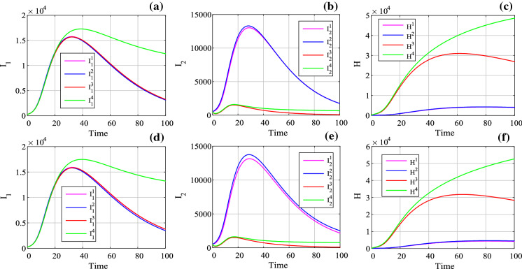
Figure 12 shows the evolution of the system with different parameters. The parameters used the Set D, and different colors lines in the figure including magenta color lines (M), blue color lines (B), red color lines (R) and green color lines (G) are obtained using the following parameters:

• M$\lambda =0.0004$, $\phi =0.009$, $\alpha =0.0$,
• B$\lambda =0.04$, $\phi =0.009$, $\alpha =0.0$,
• R$\lambda =0.0004$, $\phi =0.8$, $\alpha =0.0$,
• G$\lambda =0.04$, $\phi =0.8$, $\alpha =0.5$.

It shows that the number of infected class ($I_1$, $I_2$) and hospitalized class (H) is different with different parameters. When $\phi =0.0009$, there is a peak value for $I_2$. It means that if the hospital reception capacity is limited, the infected class ($I_2$) will increase dramatically. However, when $\phi =0.8$, the infected class ($I_2$) keeps a relative low level; thus, the infection can be controlled well. As shown in Fig. 12, when $\alpha =0.5$, it is quite difficulty for the system to become convergent. The reason is obvious because those recovered can be infected again, and a closed loop system is observed. Because no reports show that the recovered class is immune to the COVID-19, we need to be aware of those recovered to be infected again. Here, the evolution of the system with parameters of set E is shown in Fig. 13, which shows how all the classes of the system affect the dynamics. Generally, all the classes except the recovered class R will converge to zero. However, Fig. 13 is simulated with external input $\Lambda =100$ and $\alpha =0.5$. Since there is no evidence that the recovered class is immune to the virus, this makes the system hard to converge. Thus, it shows in Fig. 13 that these variables converge to zero slowly.

Fig. 12.

Evolution of the system with different parameters. a $I_1$ with $\Lambda =10$; b $I_2$ with $\Lambda =10$; c H with $\Lambda =10$; d $I_1$ with $\Lambda =100$; e $I_2$ with $\Lambda =100$; f H with $\Lambda =100$

Fig. 13.

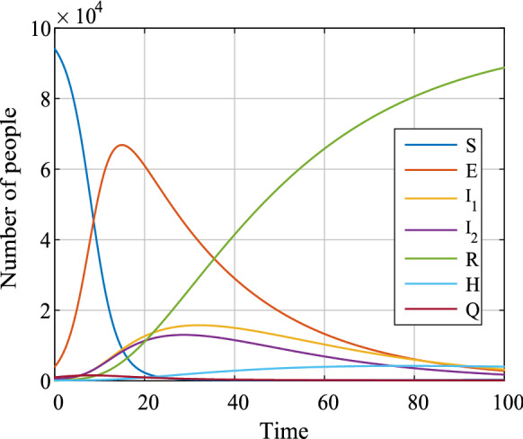
Evolution of the system with parameters of set E

In the early stage of the COVID-19 epidemic, the epidemic situation in Hubei province presents an uncontrollable trend. However, due to the low population contact rate, high hospitalization rate and high cure rate, the epidemic was quickly controlled after 20 days. Therefore, the government’s attention, people’s self-awareness and sufficient medical resources are the key to eliminate the threat of COVID-19.

To get better estimation results, we need to built a proper model and also need to set proper parameters for the systems. To the knowledge of authors, the parameters of the system change as time since the control from the government is different along with time. Thus, we can also treat the parameters as functions of time. If the values of ${\beta }_1$, ${\beta }_2$ and $\chi$ are large, the system can even become chaotic. When ${\rho }_2$ takes larger values, it means that there are more people which have like COVID-19-symptoms. In fact, the government should take stronger and harsher measures to increase isolation, especially there are many potential infections. Meanwhile, if the quarantine is done well, the values of ${\beta }_1$, ${\beta }_2$ and $\chi$ will be also much smaller; thus, it is helpful to control the spread of the epidemic disease.

Conclusion

In this paper, a SEIR model is proposed for the COVID-19. Parameters of the system are estimated by the PSO algorithm, and dynamics of the system is investigated. Finally, how the parameters affect the dynamics of the system is discussed and the control strategies are presented. The conclusions of this paper are given as follows.

1. The proposed model has considered the quarantine and treatment, so it is more suitable for the dynamics of the epidemic of COVID-19.

2. The PSO algorithm provides a good way for parameter estimation of the SEIR model. And according to the application to the data of Hubei province, the accuracy is acceptable. The main trends of the epidemic evolution are illustrated.

3. Nonlinear dynamics of the system is investigated by means of bifurcation diagram, MSE algorithm and 0–1 test algorithm. It shows that, for the given parameters, if there exists seasonality and stochastic infection, the system can generate chaos.

4. Some control suggestions are suggested based on the proposed model. Meanwhile, we found that the dynamics of the system is different with different sets of parameters.

Compliance with ethical standards

Conflict of interest

The authors declare that they have no conflict of interest.

References

- 1.Chen Y, Liu Q, Guo D. Emerging coronaviruses: genome structure, replication, and pathogenesis. J. Med. Virol. 2020;92:418–423. doi: 10.1002/jmv.25681. [DOI] [PMC free article] [PubMed] [Google Scholar]
- 2.Spaan WJM, Cavanagh D, Horzinek MC. Coronaviruses: structure and genome expression. J. General Virol. 1988;69:2939–52. doi: 10.1099/0022-1317-69-12-2939. [DOI] [PubMed] [Google Scholar]
- 3.Zhu N, Zhang D, Wang W, et al. A novel coronavirus from patients with pneumonia in china, 2019. New Engl. J. Med. 2020;382:727–733. doi: 10.1056/NEJMoa2001017. [DOI] [PMC free article] [PubMed] [Google Scholar]
- 4.Shimizu K. 2019-ncov, fake news, and racism. Lancet. 2020;395:685–686. doi: 10.1016/S0140-6736(20)30357-3. [DOI] [PMC free article] [PubMed] [Google Scholar]
- 5.Kock RA, Karesh W, Veas F, Velavan TP, Simons D, Mboera LEG, Dar OA, Arruda LB, Zumla A. 2019-ncov in context: lessons learned? Lancet. Planet. Health. 2020;4:87–88. doi: 10.1016/S2542-5196(20)30035-8. [DOI] [PMC free article] [PubMed] [Google Scholar]
- 6.Ceraolo C, Giorgi FM. Genomic variance of the 2019-ncov coronavirus. J. Med. Virol. 2020;92:522–528. doi: 10.1002/jmv.25700. [DOI] [PMC free article] [PubMed] [Google Scholar]
- 7.Ji W, Wang W, Zhao X, et al. Cross-species transmission of the newly identified coronavirus 2019-ncov. J. Med. Virol. 2020;92:433–440. doi: 10.1002/jmv.25682. [DOI] [PMC free article] [PubMed] [Google Scholar]
- 8.Fanelli D, Piazza F. Analysis and forecast of covid-19 spreading in china, italy and france. Chaos Solitons Fractals. 2020;134:109761–109761. doi: 10.1016/j.chaos.2020.109761. [DOI] [PMC free article] [PubMed] [Google Scholar]
- 9.Keeling MJ, Eames KTD. Networks and epidemic models. J. R. Soc. Interface. 2005;2:295–307. doi: 10.1098/rsif.2005.0051. [DOI] [PMC free article] [PubMed] [Google Scholar]
- 10.Prasse, B., Achterberg, M.A., Ma, L. et al.: Network-based prediction of the 2019-ncov epidemic outbreak in the chinese province hubei (2020). arXiv:2002.04482 [DOI] [PMC free article] [PubMed]
- 11.van den Driessche P, Watmough J. A simple sis epidemic model with a backward bifurcation. J. Math. Biol. 2000;40:525–540. doi: 10.1007/s002850000032. [DOI] [PubMed] [Google Scholar]
- 12.Liu, J., Paré, P.E., Du, E., Sun, Z.: A networked sis disease dynamics model with a waterborne pathogen. 2019 American Control Conference (ACC), pp. 2735–2740 (2019)
- 13.Cai Y, Kang Y, Wang W. A stochastic sirs epidemic model with nonlinear incidence rate. Appl. Math. Comput. 2017;305:221–240. [Google Scholar]
- 14.Al-Rahman El-Nor Osman M, Adu IK, Yang C. A simple seir mathematical model of malaria transmission. Asian Res. J. Math. 2017;7:1–22. doi: 10.9734/ARJOM/2017/37471. [DOI] [Google Scholar]
- 15.Almeida R. Analysis of a fractional seir model with treatment. Appl. Math. Lett. 2018;84:56–62. doi: 10.1016/j.aml.2018.04.015. [DOI] [Google Scholar]
- 16.Chen, Y., Lu, P., Chang, C.: A time-dependent sir model for COVID-19. (2020) [DOI] [PMC free article] [PubMed]
- 17.Tang B, Wang X, Li Q, et al. Estimation of the transmission risk of the 2019-ncov and its implication for public health interventions. J. Clin. Med. 2020;9:462. doi: 10.3390/jcm9020462. [DOI] [PMC free article] [PubMed] [Google Scholar]
- 18.Wu JT, Leung K, Leung GM. Nowcasting and forecasting the potential domestic and international spread of the 2019-ncov outbreak originating in wuhan, china: a modelling study. Lancet (Lond. Engl.) 2020;395:689–697. doi: 10.1016/S0140-6736(20)30260-9. [DOI] [PMC free article] [PubMed] [Google Scholar]
- 19.Wang H, Wang Z, Dong Y, et al. Phase-adjusted estimation of the number of coronavirus disease 2019 cases in wuhan, china. Cell Discov. 2020;6:462. doi: 10.1038/s41421-020-0148-0. [DOI] [PMC free article] [PubMed] [Google Scholar]
- 20.Salarieh H. Chaos analysis in attitude dynamics of a flexible satellite. Nonlinear Dyn. 2018;93(3):1421–1438. doi: 10.1007/s11071-018-4269-z. [DOI] [Google Scholar]
- 21.Krysko VA. Chaotic vibrations of flexible shallow axially symmetric shells. Nonlinear Dyn. 2018;91(4):2271–2291. doi: 10.1007/s11071-017-4013-0. [DOI] [Google Scholar]
- 22.Aihara K, Suzuki H. Theory of hybrid dynamical systems and its applications to biological and medical systems. Philosoph. Trans. R. Soc. A Math. Phys. Eng. Sci. 2010;368:4893–4914. doi: 10.1098/rsta.2010.0237. [DOI] [PubMed] [Google Scholar]
- 23.Zhang, Q., Liu, C., Zhang, X.: Complexity, analysis and control of singular biological systems (2012)
- 24.He S, Fataf NAA, Banerjee S, et al. Complexity in the muscular blood vessel model with variable fractional derivative and external disturbances. Physica A. 2019;526:120904. doi: 10.1016/j.physa.2019.04.140. [DOI] [Google Scholar]
- 25.Kuznetsov Y, Piccardi C. Bifurcation analysis of periodic seir and sir epidemic models. J. Math. Biol. 1994;32:109–121. doi: 10.1007/BF00163027. [DOI] [PubMed] [Google Scholar]
- 26.He S, Banerjee S. Epidemic outbreaks and its control using a fractional order model with seasonality and stochastic infection. Physica A. 2018;501:408-407. doi: 10.1016/j.physa.2018.02.045. [DOI] [Google Scholar]
- 27.Wang D, Tan D, Liu L. Particle swarm optimization algorithm: an overview. Soft Comput. 2018;22:387–408. doi: 10.1007/s00500-016-2474-6. [DOI] [Google Scholar]
- 28.Peng Y, Sun K, He S, Peng D. Parameter identification of fractional-order discrete chaotic systems. Entropy. 2019;21:27. doi: 10.3390/e21010027. [DOI] [PMC free article] [PubMed] [Google Scholar]
- 29.Aguiar, M.S., Kooi, B.W., Stollenwerk, N.: Epidemiology of dengue fever: A model with temporary cross-immunity and possible secondary infection shows bifurcations and chaotic behaviour in wide parameter regions. Math. Model. Natural Phenomena (2008)
- 30.Sun K, Liu X, Zhu C. The 0–1 test algorithm for chaos and its applications. Chin. Phys. B. 2010;19(11):110510. doi: 10.1088/1674-1056/19/11/110510. [DOI] [Google Scholar]
- 31.He S, Sun K, Wang H. Complexity analysis and dsp implementation of the fractional-order lorenz hyperchaotic system. Entropy. 2015;17:8299–8311. doi: 10.3390/e17127882. [DOI] [Google Scholar]
- 32.Costa M, Goldberger AL, Peng CK. Multiscale entropy analysis of complex physiologic time series. Phys. Rev. Lett. 2002;6:068102. doi: 10.1103/PhysRevLett.89.068102. [DOI] [PubMed] [Google Scholar]