Staggered release policies for COVID-19 control: Costs and benefits of relaxing restrictions by age and risk

Abstract

Lockdown and social distancing restrictions have been widely used as part of policy efforts aimed at controlling the ongoing COVID-19 pandemic. Since these restrictions have a negative impact on the economy, there exists a strong incentive to relax these policies while protecting public health. Using a modified SEIR epidemiological model, this paper explores the costs and benefits associated with the sequential release of specific groups based on age and risk from lockdown and social distancing measures. The results in this paper suggest that properly designed staggered-release policies can do better than simultaneous-release policies in terms of protecting the most vulnerable members of a population, reducing health risks overall, and increasing economic activity.

Highlights

• •Uses SEIR-type epidemic models for COVID-19 with multiple age-groups.
• •Analyzes effects of staggering the release of different groups from restrictions.
• •Staggered-release policies can reduce health risks and increase economic activity.

1. Introduction

Between March 19 and April 7, various lockdown and social distancing measures were issued around the United States. Most of these restrictions were initially slated to last 30 days, after which the states reevaluated and decided on different paths forward. Since then, most states have begun some form of reopening process. While these policy choices vary from state to state, all of these restrictions apply to every member of the population uniformly. This simultaneous-release methodology ignores the importance of differential impacts of disease on various subsets of the population.

Severity and survival rates for COVID-19 infections vary significantly. They are a function of age and various comorbidities [1]. In this paper, we use documented infection–response variation to COVID-19 to design modified lockdown and social distancing restrictions that reduce overall death rates while increasing economic activity. Staggered-release policies are compared to the benchmark policy of simultaneously releasing all groups at a predetermined time. Policies are specifically evaluated on the reduction of overall death rates from the resulting projected outbreak.

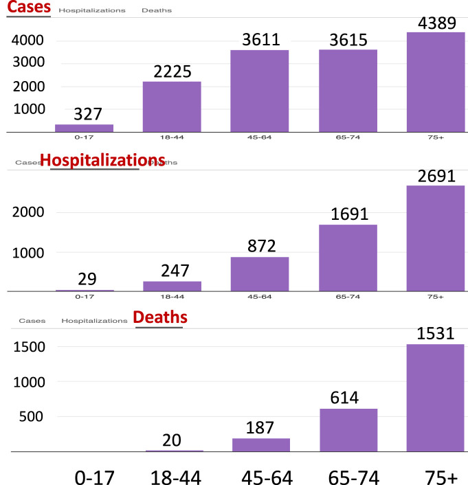
Reported data show that infected individuals over the age of 65 face a much higher case mortality than individuals under the age of 44, while those between the ages 45 and 65 have an intermediate case mortality ([2], [3], see also Fig. 1). Thus far, lockdown and social distancing restrictions have kept the overall number of deaths much lower than they would have been otherwise, particularly among the elderly. However, there are deleterious effects on the economy as well. Since restrictions were put in place in America, visits to commercial venues are down two-thirds [4], a decrease in activity that has led to small business closure and layoff rates of around 50% in the Mid-Atlantic states [5]. Shutdown sectors represent over 20% of all US payroll employment [6] and the burden of these job losses has fallen primarily on the poor [7]. All told, the economic cost of closing non-essential businesses could total nearly $10,000 per household per quarter [8], which may cause persistent harm in the form of lower output and employment and associated higher overall morbidity and mortality even after the shutdown ends [9].

Fig. 1.

COVID-19 data for New York City showing age-dependent numbers of cases (top), hospitalizations (middle), and deaths (bottom) per 100,000 people (see [2]. Accessed June 9, 2020.)

While saving lives must be the primary concern, judiciously increasing economic activity is an important secondary goal as well. Perhaps the most important result from the analysis in this paper is tied to the identification of policies that can responsibly mitigate the economic effects of a sustained shutdown without jeopardizing the most vulnerable members of the population. This paper analyzes the costs and benefits of policies that are predicated upon the timely release of younger individuals who face lower risk from COVID-19 infections from social distancing restrictions before the release of older individuals. Compared to a policy that simultaneously releases all sub-populations, carefully planned and executed staggered-release polices are likely to lead to:

• •Fewer infections over the entire duration of the outbreak
• •Lower disease mortality rate among the elderly
• •Fewer total disease deaths across the whole population
• •Increased economic activity at an earlier date

The intuition behind the merit of staggered-release policies is closely related to the ‘flattening the curve’ narrative that motivated initial public support for restrictions in the first place [1], [10]. The worst case scenario in terms of public health risk and lives lost transpires when infection rates are allowed to grow unchecked in a manner which leads to too many severe infections at once, overwhelming health care systems. Because these severe infections are much more likely among the elderly, reducing and managing elderly infection rates is a useful avenue toward improving health outcomes overall.

At the time of writing, it is believed that severe restrictions, even if maintained for an extended period of time, would be unlikely to prevent a second peak of infection since the population would not have built up significant levels of immunity before economic activity is resumed. It is strongly believed that releasing everybody at once will result in the population experiencing dramatic increases in infections, and we believe this risk may be well addressed through the usage of staggered-release policies.

This paper is organized as follows: Section 2 introduces the 3-group model and presents the setup of the benchmark and staggered-release policies. Analyses and results are presented in Section 3. Section 4 discusses the findings.

2. The three-group model and sequential release policies

Simple SIR and SEIR types of epidemic models have been used in most current studies of COVID-19 dynamics (see, for example, [11], [12], [13], [14], [15], [16], [17], [18], [19], [20]). The model introduced in this section is based on the standard Susceptible–Exposed–Infectious–Removed (SEIR) model with the incorporation of asymptomatic infections, disease-induced deaths, hospitalizations, and preferential mixing between different age groups. These modifications enable a flexible description of COVID-19 disease transmission dynamics within a model that accounts for special features associated with age-dependent groups. Since we are modeling a single outbreak, other considerations such as aging, migration, births, and unrelated deaths are ignored.

The population is divided into three groups: group 1 consisting of healthier younger people aged under 44 who have no medical conditions which may increase their risks to disease death, group 2 include people aged between 45 and 65 without health conditions, and group 3 consisting of the vulnerable members of the population including the elderly (65 years old and over) and people with higher risks than those in groups 1 and 2. These three sub-populations are labeled by $i=1,2,3$ and will be referred to as Group $i$ (or simply G1, G2, and G3). This separation of age groups is motivated by the age-specific COVID-19 data for New York presented in Fig. 1, which shows age-dependent numbers of cases, hospitalizations, and deaths per 100,000 people (see [2]), with the consideration that vulnerable people in the younger groups will be included in the high-risk group 3.

Based on available information about COVID-19, there is only a very small proportion of younger people who might have a higher risk to COVID-19 infections and deaths. Based on the US demographic data, there are about 13% of people above the age of 65, and about 25% of people between ages 45–64. Thus, the majority population is in the age group 0–44. Moving a very small proportion of the vulnerable young people into group 3 will not change much of the population size for Group 1. Each sub-population is further sub-divided into seven epidemiological classes: susceptible $\left(S_i\right)$, exposed ($E_i$), infectious but asymptomatic ($A_i$), infectious and symptomatic ($I_i$), hospitalized ($H_i$), recovered ($R_i$), and dead due to disease ($M_i$). The total population is $N={\sum }_{i=1}^3{N}_i$, where $N_i=S_i+E_i+A_i+I_i+H_i+R_i+M_i$, with $i=1,2,3$.

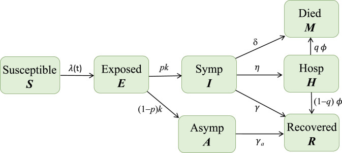
Let $k_i$ denote the per capita rate of progression to the infectious state ($1∕k_i$ represents the mean latent period), ${\gamma }_i$ and ${\gamma }_{ai}$ denote the per-capita recovery rates ($1∕{\gamma }_i$ and $1∕{\gamma }_{ai}$ are the mean infectious periods), ${\eta }_i$ denote the rate of transition from $I_i$ to $H_i$, ${\varphi }_i$ denote the rate at which hospitalized individuals leave the $H_i$ class with proportion $1-q_i$ recovered and $q_i$ dead, and ${\delta }_i$ denote the disease related death rate for individuals in the $I_i$ class. Among the infectious people, assume that proportions $p_i$ and $1-p_i$ are symptomatic and asymptomatic, respectively. Asymptomatic and hospitalized individuals can also transmit the disease but possibly at lower rates than symptomatic individuals, which are denoted by the factors ${\theta }_i\le 1$ and ${\chi }_i<1$, respectively. The parameters ${\gamma }_i,{\delta }_i$, and ${\varphi }_i$ are assumed to be independent. Other assumptions on the dependence of these parameters might also be considered, but they would not affect the qualitative conclusions of this study (see Feng et al. [21], for more detailed discussions about various underlying biological assumptions on this topic in the context of Ebola models). A disease transmission diagram for each sub-group is depicted in Fig. 2.

Fig. 2.

Depiction of disease transmission process. The infection rate $\lambda \left(t\right)$ includes transmissions from infectious people in all sub-groups. The sub-groups are connected through a mixing function given in Eq. (3).

The model is given by the following system of differential equations:

$$\begin{array}{c}{S}_i^{\prime }=-S_i{\lambda }_i\left(t\right),\hfill \\ E_i^{\prime }=S_i{\lambda }_i\left(t\right)-k_i{E}_i,\hfill \\ A_i^{\prime }=(1-p_i)k_i{E}_i-{\gamma }_{ai}{A}_i,\hfill \\ I_i^{\prime }=p_i{k}_i{E}_i-[{\gamma }_i+{\eta }_i+{\delta }_i]I_i,\hfill \\ H_i^{\prime }={\eta }_i{I}_i-{\varphi }_i{H}_i,\hfill \\ R_i^{\prime }={\gamma }_{ai}{A}_i+{\gamma }_i{I}_i+(1-q_i){\varphi }_i{H}_i,\hfill \\ M_i^{\prime }=q_i{\varphi }_i{H}_i+{\delta }_i{I}_i,i=1,2,3,\hfill \end{array}$$ (1)

where ${\lambda }_i\left(t\right)$ denotes the force of infection (FOI), the generator of new cases of infection among susceptible individuals in group $i$. The functional form of the FOI for group $i$ is given by

$${\lambda }_i\left(t\right)=\sum _{j=1}^3{a}_i\left(t\right)c_{ij}\frac{I_j+{\theta }_j{A}_j+{\chi }_j{H}_j}{N_j},i=1,2,3,$$ (2)

where $c_{ij}$ describes the mixing among the groups and defined as the proportion of the $i$th sub-group’s contacts that is with members of the $j$th group. We will adopt the commonly used preferential mixing ([22] and later extended by [23]), in which case, the elements of $C$ have the following form:

$$c_{ij}={ϵ}_i{\delta }_{ij}+(1-{ϵ}_i)f_j,\text{where}{f}_j=\frac{(1-{ϵ}_j)a_j{N}_j}{\sum _k(1-{ϵ}_k)a_k{N}_k},i,j=1,2,3,$$ (3)

where ${ϵ}_i\in [0,1]$ describes the preference level of group $i$ and ${\delta }_{ij}$ is the Kronecker delta (1 when $i=j$ and 0 otherwise). The function $c_{ij}$ in (3) satisfies the required constraints for mixing functions (see [24]). In our previous study, we estimated the mixing parameters including the age-dependent contact rates and preference levels ${ϵ}_i$ using the PolyMod data and other observations [25], which suggests that younger people tent to have higher contact rates. These results help inform our choice of model parameters in this study.

In the FOI function (2), $a_i\left(t\right)$ is the per capita effective contact rate, i.e., contacts that can lead to infection [26]. In the absence of any intervention (and no hospitalization), the group-specific basic reproduction number (i.e., without interactions with other groups) for group $i$ is

$${\mathcal{R}}_{0i}=a_{0i}\left[\frac{p_i}{{\gamma }_i}+\frac{{\theta }_i(1-p_i)}{{\gamma }_a}\right].$$

Thus, we can fix ${\mathcal{R}}_{0i}$ to get the baseline value for the effective contact rate for group $i$:

$$a_{0i}={\mathcal{R}}_{0i}∕\left[\frac{p_i}{{\gamma }_i}+\frac{{\theta }_i(1-p_i)}{{\gamma }_a}\right].$$ (4)

Note that the effective contact rate $a_{0i}$ is often expressed as a product of the contact rate with the probability of infection on contact (e.g., ${\beta }_i$). If we assume ${\beta }_i$ to be the same for all $i$ then it can be canceled in the function $f_i$ in (3). Thus, the balance condition for mixing still holds. For ease of reference, we will refer to $a_i$ simply as a contact rate.

Lockdown and social distancing restrictions are introduced to reduce the normal contact rates. Here, it is assumed that $a_i\left(t\right)$ is a function of time and that their values are influenced by the selected policy. Specifically, we model them via step functions defined as follows:

$$a_i\left(t\right)=\left\{\begin{array}{cc}\left(1-0.95s_b\right)a_{0i},\hfill & T_0\le t\le T_1,\hfill \\ \left(1-0.95s_2^{\left(i\right)}\right)a_{0i},\hfill & T_1<t\le T_2,\hfill \\ \left(1-0.95s_3^{\left(i\right)}\right)a_{0i},\hfill & T_2<t\le T_{end},\hfill \\ \left(1-0.95s_r\right)a_{0i},\hfill & t>T_{end},\hfill \end{array}\right)$$ (5)

where $T_1$, $T_2$, and $T_{end}$ represent the times when policies may change. In the case of (5), $T_0$ is the time when the initial restriction on everyone begins, $T_1$ and $T_2$ are the numbers of days from $T_0$ when Group 1 and Group 2 may be released from restrictions, respectively, and $T_{end}$ is the day from $T_0$ when the restriction for all groups is reduced to a residual level until the outbreak is over. The factor 0.95 on the severity of restrictions is meant to reflect the fact that complete isolation of every single member of a population is infeasible and likely inhumane.

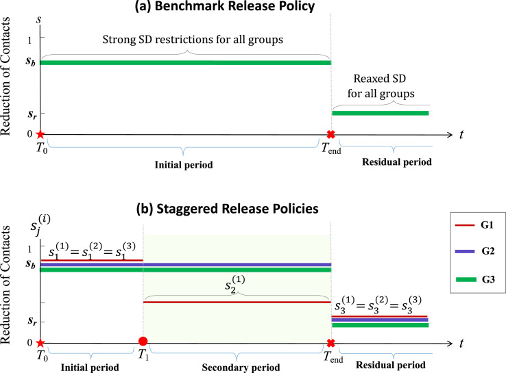
The parameters $s_j^{\left(i\right)}$ in (5) represent the reductions of contacts for group $i$ (or severity of restrictions imposed on group $i$ from business as usual (0) to no contact (1)) during the period of time $t\in (T_{j-1},T_j]$, with $i=1,2,3$ and $j=1,2,3$ ($T_3=T_{end}$). We remark that the parameters $s_j^{\left(i\right)}$ also allow us to take into consideration that a proportion of Group $i$ may not change their contacts for any reason. For example, $s_2^{\left(1\right)}$ is a weighted average of restriction levels of people in Group 1 who will or will not change their contacts during the time period $(T_1,T_2]$. To simplify notation, let $s_b$ denote the reduction of contacts during the initial restrictions, i.e., $t\in (T_0,T_1]$, and $s_r$ denote the residual restriction after the strict policies are lifted for all groups, i.e., for $t>T_{end}$. Throughout this paper, the policy corresponding to $s_j^{\left(i\right)}=s_b=0.8$ for $t\le T_{end}$ and $s_j^{\left(i\right)}=s_r=0.2$ for $t>T_{end}$, which is the case where all groups are held under the same severity of restrictions for the period $(T_0,T_{end}]$ and then all released at once at the time $T_{end}$, will be referred to as the simultaneous-release policy. We use this policy as a baseline or benchmark for evaluating the efficacy of other release policies. A staggered-release policy will be represented by relaxed restrictions for G1 at time $T_1$ and for G2 at $T_2$ with levels $s_2^{\left(1\right)},s_3^{\left(2\right)}\in [0.4,0.8]$. Examples of the schedules of the benchmark simultaneous-release policy and a staggered-release policy are depicted in Fig. 3(a) and (b), respectively. Staggered-release scenarios involving releasing Group 2 at $T_2<T_{end}$ will also be considered.

Fig. 3.

Depiction of examples showing the policy switching for the three groups. The top plot represents the benchmark simultaneous-release scenario in which all groups have restriction level $s_b$ for $T_0<t\le T_{end}$ and all groups have relaxed restriction level $s_r<s_b$ for $t>T_{end}$. The bottom diagram corresponds to one staggered-release scenario in which the times for policy switching are at $T_1$ and $T_{end}$: all groups have the restriction level $s_b$ for $T_0<t\le T_1$ and the level $s_r$ for $t>t_{end}$, but Group 1 has a relaxed level of restriction $s_2^{\left(1\right)}\in (s_r,s_b)$ for $T_1<t\le T_{end}$.

We will explore the effects of different policies by simulating Model (1) with various schedules of relaxing restrictions prescribed by chosen paths determined by $s_j^{\left(i\right)}$, $T_i$, and $T_{end}$.

3. Analysis and results

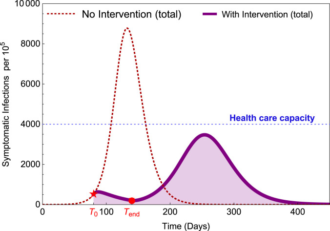
In this section, whenever we state results about staggered-release policies, they will be in terms of their performance against the benchmark delayed simultaneous-release policy. One such scenario is depicted in Fig. 4. It illustrates that when all groups are released after a long period of strong restrictions (larger $s_b$), there could be a second wave with a high peak if the residual restriction level $s_r$ is not sufficiently high and there are no other intervention measures in place to prevent it. This figure is produced by a single-group model using parameter values within the ranges listed in Table A.1.

Fig. 4.

Illustration of a potential scenario where a second wave can occur with high peak after lockdown and social distancing restrictions are relaxed. $T_0$ is the time when the restriction started and $T_{end}$ is the time when the restrictions are lifted.

Table A.1.

Definition of the symbols used in Model (1) and their values used in the examples.

Symbol	Description	Values & range
$k_i$	Rate of progression from $E_i$ to $I_i$, i.e., $1∕k_i$ is the mean latent period	(1/10, 1/7)
${\gamma }_{ai}$	Rate of recovery, i.e., $1∕{\gamma }_{ai}$ is the mean infectious period for $A$ class	(1/10, 1/5)
${\gamma }_i$	Rate of recovery, i.e., $1∕{\gamma }_i$ is the mean infectious period for $I$ class	(1/10, 1/5)
${\mathcal{R}}_{0i}$	Basic reproduction number for group $i$	(1.7, 3.6)
$a_{0i}$	Effective contact rate in the absence of intervention	See Eq. (4)
$a_i\left(t\right)$	Effective contact rate under intervention such as social distancing	See Eq. (5)
${\theta }_i$	Infectivity ratio of $A_i$ to $I_i$ individuals, $0\le {\theta }_i\le 1$	(0.3, 0.6)
${\chi }_i$	Infectivity ratio of $H_i$ to $I_i$ individuals, $0\le {\chi }_i\le 1$	(0, 0.2)
${ϵ}_i$	Level of preference for contacting one’s own group, $0\le {ϵ}_i\le 1$	(0.5, 0.9)
$c_{ij}$	Proportion of contacts a member of group $i$ has with group $j$	See Eq. (3)
${\lambda }_i\left(t\right)$	Force of infection for susceptibles in group $i$ at time $t$	See Eq. (2)
$p_i$	Proportions of infectious that are symptomatic. $p_1\le p_2\le p_3$	(0.4,0.8)
$q_i$	Proportions of disease deaths from the $H$ class	(0.00064, 0.032)
${\varphi }_i$	$1∕{\varphi }_i$ is the mean duration in $H_i$ before disease death	(0.05, 0.1)
${\delta }_i$	Rate of disease death from the $I_i$ class	(0,0.0008)
${\eta }_i$	Rate of moving from the $I_i$ class into the $H_i$ class	(0.2, 0.5)
$T_j$	Time points when a new policy starts. $T_0\le T_1\le T_2\le T_3=T_{end}$	Vary
$s_j^{\left(i\right)}$	Reduction of contacts for group $i$ in time interval $(T_{j-1},T_j]$	Vary
$s_b=s_1^{\left(i\right)}$	Reduction of contacts during the initial restrictions, i.e., in $(T_0,T_1]$	0.8
$s_r$	Reduction of contacts in the residual period $t>T_{end}$	0.2

Note: $i,j=1,2,3$. Time unit is days. Most parameter ranges are based on [1], [16], [19], [28].

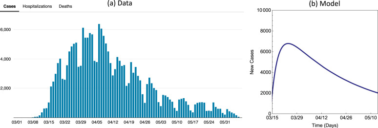
Fig. 4 is a special case of Model (1) when all groups are identical so there is only one group. We selected a value for ${\mathcal{R}}_0$ to be between the lower estimates of 2–3 (assumed in many modeling studies for COVID-19) and the high estimates such as those reported in [19], which is 5.7 (95% CI 3.8, 8.9). The value ${\mathcal{R}}_0=3.4$ provided a better match of the data of new cases shown in Fig. A.1 (see Fig. A.1 in the Appendix). Other parameter values used in this figure are ${\mathcal{R}}_0=3.4$, $p_i=0.7$, ${\gamma }_i={\gamma }_a=1∕7$, $k_i=1∕10$, ${\theta }_i=0.5$, ${\chi }_i=0.1$, $q_i=0.052$, ${\eta }_i=0.05$, ${\delta }_i=0.0006$.

Fig. A.1.

(a) Data of new cases for NYC. (b) New cases from our model.

When three groups are considered, because of the higher activity level in the younger group, ${\mathcal{R}}_{01}$ would be much higher than other groups. For given ${\mathcal{R}}_{0i}$ ($i=1,2,3$), the overall basic reproduction number ${\mathcal{R}}_0$ for the entire population can be calculated using the formula derived in the Appendix (see Appendix A.1). In most of the numerical simulations in this section, we used the values ${\mathcal{R}}_{01}=3.6$, ${\mathcal{R}}_{02}=2.7$, and ${\mathcal{R}}_{03}=2.1$, for which ${\mathcal{R}}_0=3.4$. To demonstrate that the results are not sensitive to the choice of ${\mathcal{R}}_{0i}$, examples with other lower or higher values are also included in the Appendix. Some other parameters are also assumed to have different values for the three groups. For example, $q_1=0.00064,q_2=0.008,q_3=0.032$ (i.e., Group 1 has a much lower probability of dying from COVID-19 than the older groups, as shown in Fig. 1).

We will compare the total number of disease deaths in Group $i$ from $T_0$ to the end of the outbreak under a staggered-release policy and the benchmark policy, denoted by $D_i$ and $D_{Bi}$, respectively, which can be calculated by ${\int }_{T_0}^{\infty }\left[q_i{\varphi }_i{H}_i\left(t\right)+{\delta }_i{I}_i\left(t\right)\right]dt$ (or equivalently $M_i\left(\infty \right)$) for a given policy. A staggered-release policy is evaluated based on the reductions in the cumulative deaths of group $i$ in comparison with the benchmark policy, which is termed “efficacy” and denoted by ${\mathcal{F}}_i$, i.e., 

$${\mathcal{F}}_i=\frac{D_{Bi}-D_i}{D_{Bi}},i=1,2,3.$$ (6)

Elderly and overall deaths are the primary outcomes. We will generally also present the effect of a staggered-release policy on the projected overall number of deaths in all groups, since this provides context for the possible trade-offs that occur in order to save elderly lives. Let ${\mathcal{F}}_0={\sum }_{i=1}^3{\mathcal{F}}_i$ denote the overall efficacy. Another consideration in the comparison of policies is the peak size of the total symptomatic infections.

3.1. Releasing the low-risk young group first saves lives

In this section, we analyze the costs and benefits of releasing Group 1 from restrictions before other groups. In this case, $T_2=T_{end}$. Examples of releasing all three groups at different time points are considered in Section 3.2. To identify the effects, we hold constant the total duration of restrictions and the severity of restrictions on Group 2 and elderly Group 3. At $T_1\in (T_0,T_{end})$, there is a choice of whether (and to what degree) to release Group 1 from restrictions; a choice of $s_2^{\left(1\right)}\in (s_r,s_b)=(0.2,0.8)$.

For ease of presentation, in the remainder of this paper we will shift the time axis to have $T_0=0$ (the time when the initial restriction starts) and let $T_1$ and $T_{end}$ represent the times from $T_0$. The values at $T_0$ of the state variables of the original system (1) without intervention will be taken as the initial values at $t=0$ for the shifted system. The comparisons of outcomes between staggered- and simultaneous-release scenarios will be considered based on changes after $T_0$.

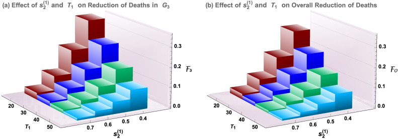
Fig. 5 presents how the efficacy for the elderly group (${\mathcal{F}}_3$) and the overall efficacy (${\mathcal{F}}_0$) vary with the policy parameters $T_1$ and $s_2^{\left(1\right)}$. Several staggered-release policies are represented by $T_1=20,30,40,50$ and $s_2^{\left(1\right)}=0.4,0.5,0.6,0.7$, while the delayed simultaneous-release policy corresponds to $T_1=T_{end}=120$ or $s_2^{\left(1\right)}=0.8$. Other parameter values are: ${\gamma }_i={\gamma }_a=0.14$, ${ϵ}_1=0.7,{ϵ}_2=0.5,{ϵ}_3=0.9$, $p_1=0.4,p_2=0.6,p_3=0.8$, ${\theta }_i=0.5$, ${\chi }_i=0.1$, $q_1=0.00064,q_2=0.008,q_3=0.032$, ${\delta }_1=0.01q_1$, ${\delta }_2=0.01q_2$, ${\delta }_3=0.025q_3$, ${\eta }_1=0.0125$, ${\eta }_2=0.05$, ${\eta }_3=0.1$. The efficacies for Group 3 and overall are illustrated in Fig. 5(a) and (b), respectively.

Fig. 5.

Dependence of the efficacy for elderly (${\mathcal{F}}_3$) and the overall efficacy (${\mathcal{F}}_0$) on the timing $T_1$ and restriction level $s_2^{\left(1\right)}$.

Results shown in Fig. 5 suggest that there is a significant reduction in elderly deaths and overall deaths as the low-risk young group faces less severe restrictions ($s_2^{\left(1\right)}$) and as this relaxation of restrictions takes place at an earlier date ($T_1$), and these responses are strictly monotonic in both $s_2^{\left(1\right)}$ and $T_1$. Particularly, the timely release of Group 1 with $s_2^{\left(1\right)}=0.4$ and $20\le T_1\le 50$ can decrease elderly and overall disease deaths by 7% to 28% of their projected values under the simultaneous-release policy, for the parameter values used. Results for different sets of parameter values are discussed in later sections.

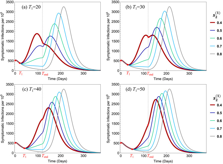
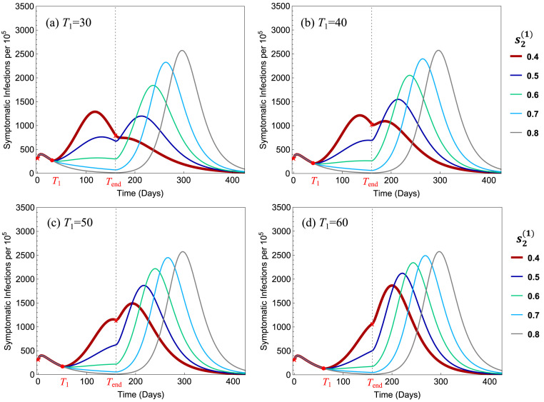
Fig. 6 illustrates the influence of the policy parameters $s_2^{\left(1\right)}$ and $T_1$ on the total symptomatic infections (per 100,000). All parameter values are the same as in Fig. 5. It shows that in all 4 plots the peak size decreases when $s_2^{\left(1\right)}$ decreased from 0.8 to 0.5, but in (a) the peak increased when $s_2^{\left(1\right)}$ is decreased further to 0.4. For $s_2^{\left(1\right)}=0.4$, the early releases of Group 1 reduce the peak size by 19%–44% in all four plots.

Fig. 6.

Dependence of the total symptomatic infections on the policy parameters $T_1$ and $s_2^{\left(1\right)}$. In all four plots, the benchmark simultaneous-release scenario corresponds to the curve with the highest peak, which corresponds to the strict restriction level $s_2^{\left(1\right)}=0.8$.

For the scenarios presented in Fig. 5, Fig. 6, we observe that the restriction level $s_2^{\left(1\right)}=0.4$ would provide the most beneficial policy for all values of $T_1$, and that $T_1=20$ and 30 are better choices than $T_1=40$ or 50. For ease of reference, we refer to these two policies as:

• • Policy I: $T_1=30$ and $s_2^{\left(1\right)}=0.4$;
• • Policy II: $T_1=20$ and $s_2^{\left(1\right)}=0.4$.

If we compare Policy I and Policy II, both have advantages and disadvantages. Policy I has a relatively lower peak size (see the thicker-red curve in Fig. 6(a) and (b)) while Policy II leads to higher efficacies (see the red column in Fig. 5(a) and (b)). Examples of policies with $s_2^{\left(1\right)}<0.4$ will be discussed later.

Additional simulations of Model (1) with a wider range of parameter values show similar qualitative behavior, some of which are included in the following sections and in Appendix. Particularly, the main results are not sensitive to the choices of group-specific and overall basic reproduction numbers (${\mathcal{R}}_{0i}$ and ${\mathcal{R}}_0$), proportions of symptomatic infections ($p_i$), mean infectious period ($1∕\gamma$), and $T_{end}$. The following results summarize how the reductions in disease deaths (${\mathcal{F}}_i$) for the elderly group and overall respond to the early release of Group 1 from restrictions.

Result 1. The following results are based on a large number of simulations of Model (1) with a broader range of reasonable parameter values for COVID-19.

• (i) Both the overall efficacy ${\mathcal{F}}_0$ and the efficacy for the most vulnerable and elderly group ${\mathcal{F}}_3$ are strictly increasing as the severity of secondary restriction level $s_2^{\left(1\right)}$ decreases.
• (ii) The peak size of the total symptomatic infections may be the lowest at an intermediate value of severity $s_2^{\left(1\right)}\in (s_r,s_b)$.
• (iii) For smaller $s_2^{\left(1\right)}>s_r$, the efficacy ${\mathcal{F}}_1$ for Group 1 may become negative if the disease mortality for Group 1 is high.

In all simulated results, staggered-release policies are more beneficial than the simultaneous-release benchmark policy in the sense that they help reduce disease deaths in the most vulnerable population and lower the peak size, while allowing increased economic activities.

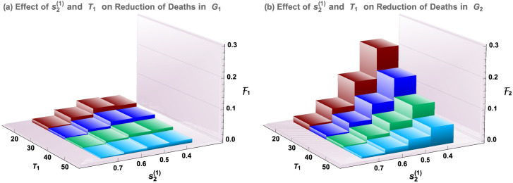
Results presented in Fig. 5, Fig. 6 suggest that, in the evaluation of staggered-release policies, balanced considerations are needed between reductions of disease deaths and the peak size of symptomatic infections. We may also consider the efficacies for Groups 1 and 2. This is presented in Fig. 7. We observe that the behavior of ${\mathcal{F}}_2$ as shown in Fig. 7(b) is very similar to that of Group 3 as shown in Fig. 5(a), while Fig. 7(a) shows that the changes of disease deaths for Group 1 are much smaller. This is because the disease mortality for Group 1 is much lower. Parameter values are the same as in Fig. 5.

Fig. 7.

Similar to Fig. 5 but for Groups 1 and 2. All parameter values are the same as in Fig. 5.

3.2. Fully staggered releases require proper timing

Results in the previous sections present the positive impacts of releasing Group 1 before the other two groups are released at the same time. In this section, we explore the impact of relax restrictions for Group 2 at some point before the final releases of all groups at $T_{end}$. The intuition would be that since Group 2 is less vulnerable than Group 3, staggering their releases may have similar benefits to the early release of Group 1 only. We will observe a similar result here, but with some caveats.

Let $T_2$ represent the timing for releasing Group 2 with a restriction level $s_3^{\left(2\right)}$. As before, the restriction level for Group 3 will be kept at 0.8 for all $t<T_{end}$, but now $s_3^{\left(2\right)}$ is another policy variable. Assume that the severity level for Group 1 does not change in $(T_2,T_{end}]$, i.e., $s_2^{\left(1\right)}=s_3^{\left(1\right)}$. As more detailed analysis of the degree of Group 1 release, $s_2^{\left(1\right)}$, and the timing $T_1$ have already been done in the previous sections, in this section we will fix $s_2^{\left(1\right)}=0.4$ and $T_1=30$. We will vary the cutoff time $T_2$ and the severity $s_3^{\left(2\right)}\in [0.4,0.8]$. Note that the staggered policy considered in the previous section corresponds to $(T_1,T_2,T_{end})=(30,120,120)$. We refer to this as the “G1-release” policy. The baseline simultaneous-release policy will be the same idea as before, with all three groups being held under the same initial restrictions until $T_{end}$. This is represented by $T_1=T_2=T_{end}=120$ with $s_2^{\left(1\right)}=s_3^{\left(2\right)}=0.8$.

Two natural comparisons are the “G1-release” policy and the “G2-release” policy with $T_1<T_2<T_{end}$. One example is illustrated in Fig. 8, in which $T_1=30$, $T_2=60$, $s_2^{\left(1\right)}=0.4$, with various values of $s_3^{\left(2\right)}$. All other parameter values are the same as in Fig. 5, Fig. 6.

Fig. 8.

Comparison of the G1-release and G2-release policies represented by the solid and dashed curves, respectively, in (a) and (b). The efficacies for Group 3 and overall are shown in (c) for four values of $s_3^{\left(2\right)}$, where $s_3^{\left(2\right)}=0.4$ and 0.8 correspond to the G1-release and G2-release, respectively.

We observe from Fig. 8(a) that the G2-release ($s_3^{\left(2\right)}=0.4$) has a higher peak size than the G1-release ($s_3^{\left(2\right)}=0.8$), although both peaks are much lower than that of the simultaneous-release. Fig. 8(b) shows that the increased infections of the G2-release resulted in an increased number of disease deaths in Group 2, particularly during an earlier period of the outbreak. Plot (c) shows that the early release of Group 2 generated slightly higher efficacy in the elderly group 3 but decreased the overall efficacy, which is due to the increased deaths in Group 2. The changes in peak size, number of deaths, and efficacy vary with the timing $T_2$. This suggests that a careful selection of $T_2$ and a more detailed cost-benefit analysis should be carried out to determine the most beneficial policies for releasing Group 2.

3.3. Robustness of the simulation results

In most of our simulations of Model (1) using a broad range of parameter values, the qualitative behavior concerning the efficacies ${\mathcal{F}}_i$ and the peak sizes of symptomatic infections are similar. Several examples are provided in this section and in the Appendix.

Fig. 9 illustrates results for reduced group reproduction numbers: ${\mathcal{R}}_{01}=3,{\mathcal{R}}_{02}=2.25$, and ${\mathcal{R}}_{02}=1.75$. All other parameters are the same as in Fig. 5, Fig. 6 with $T_1=20$ and $T_{end}=150$. As $s_2^{\left(1\right)}$ decreases from 0.8 to 0.4, plot (a) shows that the peak size is the lowest at $s_2^{\left(1\right)}=0.5$; plot (b) shows that the cumulative numbers of deaths decrease monotonically in Groups 2 and 3 but remains almost the same in Group 1; and plot (c) presents the corresponding efficacies ${\mathcal{F}}_i$ for all groups. These plots show a similar qualitative behavior as in Fig. 5, Fig. 6 (see the case of $s_2^{\left(1\right)}=0.4$ and $T_1=20$).

Fig. 9.

Influence of the policy parameter $s_2^{\left(1\right)}$ on (a) symptomatic infections, (b) cumulative disease deaths, and (c) Efficacies ${\mathcal{F}}_i$.

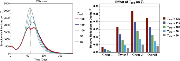
To explore the influence of $T_{end}$, Fig. 10 illustrates the results for $T_{end}=80,90,100,110,120$. All other parameters are the same as in Fig. 5, Fig. 6 with $T_1=30$ and $s_2^{\left(1\right)}=0.4$. It shows that, as $T_{end}$ decreases, the peak size increases while the efficacy ${\mathcal{F}}_i$ decreases within each group. One of the reasons for the larger peak size for smaller $T_{end}$ values (e.g., 80–100) is because the number of infections are still in the increasing phase at the time of releasing all groups, whereas for $T_{end}=120$ the infection curve has already started decreasing. This suggests that the timing of group releases can be critically important.

Fig. 10.

Effects of $T_{end}$ on the efficacy ${\mathcal{F}}_i$ with fixed $T_1=30$ days and $s_2^{\left(1\right)}=0.4$. All other parameters are the same as in Fig. 5, Fig. 6.

The significantly lower case mortality for the younger groups shown in Fig. 1 was considered in the choice for values of $q_i$ for the figures in previous sections. If, however, in a different population $q_1$ is not so much lower than $q_2$ and $q_3$, a more detailed cost and benefit analysis might be needed in the examination of policies for releasing Group 1 earlier. In Fig. 11, the values $q_1=0.0016$, $q_2=0.008$, $q_3=0.032$ are used. All other parameters are the same as in Fig. 5, Fig. 6 with $T_1=30$, and an additional of $s_2^{\left(1\right)}=0.2$ is included in the comparison. One key difference between the results shown in Fig. 11 and others presented earlier is that, the least strict restriction ($s_2^{\left(1\right)}=0.2$) may shift the peak earlier in time with a much higher peak size than the case of $s_2^{\left(1\right)}=0.4$ (see (a)). On one hand, this can greatly increase the population immunity, which may reduce the loss of life in the elderly group 3 (see (b)) and increase the efficacies for both Group 3 and overall (see (c)). On the other hand, however, the efficacy ${\mathcal{F}}_1$ for Group 1 is negative for $s_2^{\left(1\right)}=0.2$ (see (c)), which represents increased deaths in Group 1, although by a very small number. This can be avoided by restricting $s_2^{\left(1\right)}$ to be higher than 0.2 to ensure non-negative ${\mathcal{F}}_1$, as done in the earlier examples.

Fig. 11.

Similar to Fig. 9 but for $q_1=0.0016$, $T_1=30$. The values of ${\mathcal{R}}_i$ are the same as in Fig. 5 and an additional value of $s_2^{\left(1\right)}=0.2$ is included.

4. Discussion

The findings generated by a careful study of various scenarios support the view that releasing some appropriately defined groups earlier from lockdown and social distancing restrictions may be highly beneficial under the premise that reducing overall disease deaths is the priority. The use of a staggered-release policy built on the immunological strength of sub-groups of a population may indeed prove to be highly effective in terms of protecting vulnerable individuals while mitigating economic setbacks.

Staggered-release policies are designed to avoid dangerous levels of severe infections among the most vulnerable by redistributing the timing and likelihood of infection across groups. The release of low-risk and young from restrictions earlier might increase their disease exposure, but most infections would be asymptomatic or mild. The second group would be then released after some level of population immunity has been achieved among the first group. The related concept of deploying recovered individuals with antibodies into society to restart the economy while keeping infectious contacts low has been put forward in Weitz et al. [27], who term it ‘shield immunity.’

The effectiveness of staggered-release policies is crucially tied to timing choices. We show that the mistimed release of groups may lead to an increase in overall disease deaths. While the early release of the youngest group is generally going to be significantly helpful, the response of the epidemic curve to specific choices of when to release older groups is complicated, as pointed out more generally by Morris et al. [17].

Simulations show that if the second group’s release is timed to take place just before the peak of infections, then the release may lead to a higher peak of infections and more disease deaths. On the other hand, releasing this second group after the peak of infections generated by the first group has passed produces only a small or no bump in infections that does not increase significantly the risks of those involved, a result consistent with the findings in Morris et al. [17]. Morris et al. observe that optimal control in this context responds to changing levels of susceptibility and infection rates in the population.

Compared to the delayed simultaneous-release benchmark, staggered-release policies that release Group 1 first can save a significant portion of lives among the elderly. In most of the examples presented in this paper, we see commonly 10%–20% reduction in elderly disease deaths compared to the simultaneous-release policy. The estimated size of this effect is robust to alternate parameter specifications.

Results shown in Fig. 10, Fig. A.3 reveal a stark change in outcomes if the release of older groups is mistimed, even if it is carried out a few weeks too early. Releasing these individuals from restrictions while infections are still rising results in a significantly higher peak size of symptomatic infections compared to those from a policy of waiting to release them only after infections have begun to fall.

Fig. A.3.

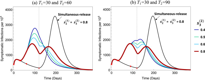
Symptomatic infections under four different policies corresponding to $s_3^{\left(2\right)}=0.4,0.5,0.6,0.8$ with (a) $T_1=30,T_2=60$ and (b) $T_1=30$ and $T_2=90$. Both plots are for $s_2^{\left(1\right)}=0.4$ and $T_{end}=120$. The benchmark simultaneous-release policy ($s_2^{\left(1\right)}=s_3^{\left(2\right)}=0.8$) is also plotted. Plot (a) shows a much higher peak size than plot (b) for $s_3^{\left(2\right)}=0.4$.

Importantly, while economic considerations were mentioned as a motivating factor behind the earlier removal of restrictions for some groups, there were no actual economic components in the model we used in this paper. Our conclusion that staggered-release policies outperform simultaneous-release policies is shown through a direct comparison of health risks and aggregate loss of life estimated from projections of the outbreak under these policies. The fact that earlier release of certain sub-groups enhances economic activity on the whole is a further benefit to staggered-release policies, but this is a benefit that exists outside of our model.

It would be insightful to incorporate the adverse health consequences associated with lengthy lockdown restrictions, such as increased risk of depression and loss of health insurance from employment to cover unrelated medical issues, within the comparison structure used in this paper. However, we wanted the focus to be on a direct comparison of health risks associated with the disease itself, so that it is clear that these additional consequences do not drive the result. We leave the explicit consideration of these additional health risks to future work.

Ultimately, it was our goal to analyze the use of staggered-release policies and compare the outcomes to those resulting from a policy of the delayed simultaneous release of everyone. This is meant to be an illustrative paper, not a prescriptive one. Implementing staggered-release policies would require a more thorough analysis of the specific population under consideration in order to appropriately structure the schedule of release.

4.1. Conclusion

Lockdown and social distancing restrictions have been an important tool in controlling the spread of COVID-19 and keeping infection rates low enough to avoid exceeding health care capacity. Now that the initial phase of the outbreak has been addressed, the next step is to properly schedule the relaxation of constraints in order to optimally control the entirety of the outbreak. The decision to lift restrictions on everyone simultaneously is perhaps the natural policy, but this can have dire consequences if a second peak arises as a result of insufficient immunity in the population. Such an outcome would defeat the purpose of installing restrictions in the first place, so it is crucially important to consider more effective policies in terms of when to release people from restrictions.

To summarize, the early release of low-risk young individuals provides an interim period that allows them to build up some degree of immunity without facing significant health risks themselves, in order to protect older and more vulnerable individuals from severe health risks by reducing their likelihood of infection and death. As an added benefit, the staggered-release policy allows for more activity in the population at an earlier date than the delayed simultaneous-release policy would. Thus staggered-release policies can positively impact everyone involved by allowing people to return to their lives without risking them.

Declaration of Competing Interest

The authors declare that they have no known competing financial interests or personal relationships that could have appeared to influence the work reported in this paper.

Appendix.

In this appendix, we include the derivation of the basic reproduction number of the 3-group model (1) and present several examples to demonstrate that the main conclusions discussed in this paper are not sensitive to the choice of those model parameters that may have higher levels of uncertainty. These include the proportions of symptomatic infections ($p_i$), the recovery rate (${\gamma }_i$), and group-specific basic reproduction numbers ${\mathcal{R}}_{0i}$.

A.1. Basic reproduction number of model (1)

Let $\mathbf{v}$ denote the vector of infected state variables (without hospitalization) in the following order:

$$\mathbf{v}=(E_1,A_1,I_1,E_2,A_2,I_2,E_3,A_3,I_3)$$

and consider the system for fractions of these variables within each group (e.g., $x_i=E_i∕N_i$, $y_i=A_i∕N_i$, $z_i=I_i∕N_i$, $i=1,2,3$). Let

$$T_i=\frac{p_i}{{\gamma }_i+{\mu }_i}+{\theta }_i\frac{1-p_i}{{\gamma }_a},i=1,2,3.$$

Then, the group-specific basic reproduction number for group $i$ is

$${\mathcal{R}}_{0i}=a_{0i}{T}_i=a_{0i}\left[\frac{p_i}{{\gamma }_i+{\mu }_i}+{\theta }_i\frac{1-p_i}{{\gamma }_a}\right].$$ (7)

For the whole population, the next generation matrix is a 3 × 3 block matrix $K=\left(K_{ij}\right)$ with

$$K_{ij}=\left(\begin{array}{ccc}\hfill a_{0i}{T}_j{c}_{ij}\hfill & \hfill \ast \hfill & \hfill \ast \hfill \\ \hfill 0\hfill & \hfill 0\hfill & \hfill 0\hfill \\ \hfill 0\hfill & \hfill 0\hfill & \hfill 0\hfill \end{array}\right)\text{for}i,j=1,2,3,$$

where the “*” entries do not affect the result. The non-zero eigenvalues of $K$ are given by the following matrix:

$$H=\left(\begin{array}{ccc}\hfill a_{01}{T}_1{c}_{11}\hfill & \hfill a_{01}{T}_2{c}_{12}\hfill & \hfill a_{01}{T}_3{c}_{13}\hfill \\ \hfill a_{02}{T}_1{c}_{21}\hfill & \hfill a_{02}{T}_2{c}_{22}\hfill & \hfill a_{02}{T}_3{c}_{23}\hfill \\ \hfill a_{03}{T}_1{c}_{31}\hfill & \hfill a_{03}{T}_2{c}_{32}\hfill & \hfill a_{03}{T}_3{c}_{33}\hfill \end{array}\right).$$

Let $\rho \left(H\right)$ denote the dominant eigenvalue of $H$, then the basic reproduction number for the whole population is given by

$${\mathcal{R}}_0=\rho \left(H\right).$$ (8)

For the parameter values used in Fig. 5, Fig. 6, ${\mathcal{R}}_0=3.4$.

A.2. Choice of parameter values

Most of the simulations in this study used parameter values motivated by the data for New York City (see [2]). Fig, A.1 demonstrates that the new cases generated by these values are on a similar order to that observed in data. This figure is produced by the same model that generated Fig. 5, Fig. 6 in the case of a homogeneous population (assumed same contact rates and other parameters for all groups) for $t$ between 03/15 and 5/13 with $s_b=0.8$. For other parameter values, using the data shown in Fig. 1 we get the following estimates used to produce Fig. A.1(b): ${\mathcal{R}}_{0i}={\mathcal{R}}_0=3.4$, $p_i=0.7$, ${\gamma }_i={\gamma }_a=1∕7$, $k_i=1∕10$, ${\theta }_i=0.5$, ${\chi }_i=0.1$, $q_i=0.052$, ${\eta }_i=0.05$, ${\delta }_i=0.0006$. The case numbers are scaled to 8.4 million total population size for NYC.

A.3. Proportion of symptomatic infections and infectious period

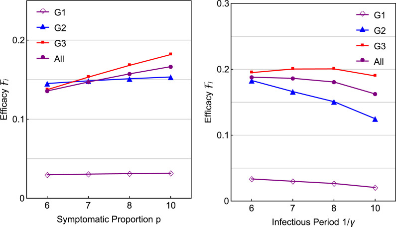
Fix all other parameter as in Fig. 5 with $T_1=30$ and $s_2^{\left(1\right)}=0.4$. Consider two sets of $p_i$ and ${\gamma }_i$: (i) $p_i=p=0.5,0.6,0.7,0.8$ and $1∕{\gamma }_i=7$, and (ii) $1∕{\gamma }_i=1∕\gamma =6,7,8,10$ with $p_i$ being the same as in Fig. 5. Results are presented in Fig. A.2. We observe that the efficacies for the elderly and overall are very similar for different values of $p_i$ or ${\gamma }_i$.

Fig. A.2.

Effects of the proportion of symptomatic infections $p_i$ and the infectious period $1∕\gamma$ on the efficacy ${\mathcal{F}}_i$ with fixed $T_1=30$ days and $s_2^{\left(1\right)}=0.4$. All other parameters are the same as in Fig. 5, Fig. 6.

A.4. Group-specific basic reproduction numbers

First, consider the group-specific basic reproduction numbers: ${\mathcal{R}}_{01}=4.8$, ${\mathcal{R}}_{02}=3.6$, ${\mathcal{R}}_{03}=2.4$, which are higher than those used in Fig. 5. All other parameter values are the same as in Fig. 5, Fig. 6 with $T_1=30$ days and $s_2^{\left(1\right)}=0.4$. Fig. A.3 illustrates numerical results of two scenarios of G2-release: (a) $T_2=60,T_{end}=120$, and $s_3^{\left(2\right)}=0.4,0.5,0.6,0.8$; and (b) $T_2=90$ and other parameters are the same as in (a). We observe in (a) that the peak size increases as $s_3^{\left(2\right)}$ decreases from 0.8 to 0.4, whereas in (b) the increase of the peak size is not as large as in (a). This demonstrates a similar behavior as in Fig. 10. That is, the reason for the higher peak sizes in (a) is because at the time of release ($T_2=60$) of Group 2 the infections are still increasing, which is not the case in (b).

Next, consider the group-specific reproduction numbers: ${\mathcal{R}}_{01}=3.18$, ${\mathcal{R}}_{02}=2.39$, ${\mathcal{R}}_{03}=1.86$, which are lower than those used in Fig. 5. In this case ${\mathcal{R}}_0=3$ (see Eqs. (7), (8) in Appendix A.1). All other parameters are the same as in Fig. 5, Fig. 6 except that $T_{end}=160$. Fig. A.4 shows that the effect of $s_2^{\left(1\right)}$ on the infection curves is very similar to that shown in Fig. 6. The efficacies ${\mathcal{F}}_3$ and ${\mathcal{F}}_0$ also show similar properties as in Fig. 5 (omitted here).

Fig. A.4.

Similar to Fig. 6 but for lower values of ${\mathcal{R}}_{0i}$ and $T_{end}=160$.

References

- 1.CDC . 2020. Coronavirus (COVID-19)https://www.cdc.gov/coronavirus/2019-ncov/index.html [Google Scholar]
- 2.NYC Health . 2020. COVID-19 Data.https://www1.nyc.gov/site/doh/covid/covid-19-data.page [Google Scholar]
- 3.Elflein J. Percentage of COVID-19 cases in the United States from February 12 to March 16, 2020 resulting in death, by age group. Statista. 2020 https://www.statista.com/statistics/1105431/covid-case-fatality-rates-us-by-age-group/ [Google Scholar]
- 4.Couture V., Dingle J., Green A., Handbury J., Williams K. 2020. COVID Exposure indices.https://github.com/COVIDExposureIndices/ [Google Scholar]
- 5.Bartik A., Bertrand M., Cullen Z., Glaeser E., Luca M., Stanton C. Becker Friedman Institute; 2020. How are Small Businesses Adjusting To COVID-19? Early Evidence from a Survey: Working Paper. [Google Scholar]
- 6.Vavra J. U.S. Bureau of Labor Statistics; 2020. How Many Workers are Employed in Sectors Directly Affected by COVID-19 Shutdowns, where Do they Work, and how Much Do they Earn? [Google Scholar]
- 7.Mongey S., Phillosoph L., Weinberg A. Becker Friedman Institute; 2020. Which Workers Bear the Burden of Social Distancing Policies?: Working Paper. [Google Scholar]
- 8.Mulligan C. The economic cost of shutting down “non-essential”. Businesses. 2020 [Google Scholar]
- 9.Huber K. Disentangling the effects of a banking crisis: Evidence from German firms and counties. Amer. Econ. Rev. 2020;108:868–898. doi: 10.1101/2020.04.17.20069351. [DOI] [Google Scholar]
- 10.Qualls N., Levitt A., Kanade N. Community mitigation guidelines to prevent pandemic influenza–United States. MMWR Recommendations Rep. 2017;66:1–34. doi: 10.15585/mmwr.rr6601a1. [DOI] [PMC free article] [PubMed] [Google Scholar]
- 11.Acuña-Zegarra M.A., Santana-Cibrian M., Velasco-Hernandez J.X. Modeling behavioral change and COVID-19 con- tainment in Mexico: A trade-off between lockdown and compliance. Math. Biosci. 2020;325:108370. doi: 10.1016/j.mbs.2020.108370. [DOI] [PMC free article] [PubMed] [Google Scholar]
- 12.Ferguson N.M. Imperial College; London: 2020. Impact of Non-Pharmaceutical Interventions (NPIs) to Reduce COVID-19 Mortality and Healthcare Demand. [DOI] [PMC free article] [PubMed] [Google Scholar]
- 13.Gupta R. 2020. SEIR and Regression Model Based COVID-19 Outbreak Predictions in India. [DOI] [Google Scholar]
- 14.Kucharski A.J. Of transmission and control of COVID-19: a mathematical modelling study. Lancet Infect. Dis. [Internet] 2020 doi: 10.1016/S1473-3099(20)30144-4. 3099(20):2020.01.31.20019901, Available from: http://medrxiv.org/content/early/2020/02/18/2020.01.31.20019901.abstract. [DOI] [PMC free article] [PubMed] [Google Scholar]
- 15.Li Q., Tang B., Bragazzi N.L., Xiao Y., Wu J. Modeling the impact of mass influenza vaccination and public health interventions on COVID-19 epidemics with limited detection capability. Math. Biosci. 2020;325:108378. doi: 10.1016/j.mbs.2020.108378. [DOI] [PMC free article] [PubMed] [Google Scholar]
- 16.Li R., Pei S., Chen B., Song Y., Tao Z., Wang W., Shaman J. Substantial undocumented infection facilitates the rapid dissemination of novel coronavirus (SARS-CoV2) Science. 2020:eabb3221. doi: 10.1126/science.abb3221. [DOI] [PMC free article] [PubMed] [Google Scholar]
- 17.Morris D.H., Rossine F.W., Plotkin J.B., Levin S.A. 2020. Optimal, near-optimal, and robust epidemic control. arXiv:2004.02209v2 [Preprint] [Google Scholar]
- 18.Ngonghala C.N., Iboi E., Eikenberry S., Scotch M., Gumel A.B. Mathematical assessment of the impact of non-pharmaceutical interventions on curtailing the 2019 novel Coronavirus. Math. Biosci. 2020;325:108364. doi: 10.1016/j.mbs.2020.108364. [DOI] [PMC free article] [PubMed] [Google Scholar]
- 19.Sanche S. High contagiousness and rapid spread of severe acute respiratory syndrome Coronavirus 2. Emerg. Infect. Diseases. 2020;26 doi: 10.3201/eid2607.200282. [DOI] [PMC free article] [PubMed] [Google Scholar]
- 20.Xue L., Jing S., Miller J.C., Sun W., Li H., Estrada-Franco J.G., Hyman J.M., Zhu H. A data-driven network model for the emerging COVID-19 epidemics in Wuhan, Toronto and Italy. Math. Biosci. 2020;326:108391. doi: 10.1016/j.mbs.2020.108391. [DOI] [PMC free article] [PubMed] [Google Scholar]
- 21.Feng Z., Zheng Y., Hernandez-Ceron N., Zhao H., Glasser J.W., Hill A.N. Mathematical models of Ebola - Consequences of underlying assumptions. Math. Biosci. 2016;277:89–107. doi: 10.1016/j.mbs.2016.04.002. [DOI] [PubMed] [Google Scholar]
- 22.Nold A. Heterogeneity in disease transmission modeling. Math. Biosci. 1980;124:59–82. [Google Scholar]
- 23.Jacquez J.A., Simon C.P., Koopman J., Sattenspiel L., Perry T. Modeling and analyzing HIV transmission: the effect of contact patterns. Math. Biosci. 1988;92:119–199. [Google Scholar]
- 24.Busenberg S., Castillo-Chavez C. A general solution of the problem of mixing of sub-populations and its application to risk- and age-structured epidemic models for the spread of AIDS. IMA J. Math. Appl. Med. Biol. 1991;8 doi: 10.1093/imammb/8.1.1. [DOI] [PubMed] [Google Scholar]
- 25.Glasser J.W., Feng Z., Moylan A., Del Valled S., Castillo-Chavez C. Mixing in age-structured population models of infectious diseases. Math. Biosci. 2012;235:1–7. doi: 10.1016/j.mbs.2011.10.001. [DOI] [PubMed] [Google Scholar]
- 26.Hethcote H.W. The mathematics of infectious diseases. SIAM Rev. 2000;42:599–653. [Google Scholar]
- 27.Weitz J.S. 2020. Intervention serology and interaction substitution: Modeling the role of ‘shield immunity’ in reducing COVID-19 epidemic spread. [DOI] [Google Scholar]
- 28.CDC . 2020. COVID-19 case surveillance public use data.https://data.cdc.gov/Case-Surveillance/COVID-19-Case-Surveillance-Public-Use-Data/vbim-akqf [Google Scholar]