Prediction of Heart Transplant Rejection Using Histopathological Whole-Slide Imaging

Abstract

Endomyocardial biopsies are the current gold standard for monitoring heart transplant patients for signs of cardiac allograft rejection. Manually analyzing the acquired tissue samples can be costly, time-consuming, and subjective. Computer-aided diagnosis, using digitized whole-slide images, has been used to classify the presence and grading of diseases such as brain tumors and breast cancer, and we expect it can be used for prediction of cardiac allograft rejection. In this paper, we first create a pipeline to normalize and extract pixel-level and object-level features from histopathological whole-slide images of endomyocardial biopsies. Then, we develop a two-stage classification algorithm, where we first cluster individual tiles and then use the frequency of tiles in each cluster for classification of each whole-slide image. Our results show that the addition of an unsupervised clustering step leads to higher classification accuracy, as well as the importance of object-level features based on the pathophysiology of rejection. Future expansion of this study includes the development of a multiclass classification pipeline for subtypes and grades of cardiac allograft rejection.

I. INTRODUCTION

Endomyocardial biopsies are the current gold standard when monitoring heart transplant patients for signs of cardiac allograft rejection [1]. Biopsies are repeated at varying frequencies following transplantation and allow for an empirical method to diagnose rejection, allowing for monitoring and recognizing the need for treatment of cardiac allograft rejection. Accurate classification of rejection status can ultimately improve heart transplant patient outcomes by optimizing immunosuppressive therapy [1]. Rejection surveillance, which can allow for a more timely diagnosis and treatment plan, is especially important for heart transplant patients, as most of the heart transplant patients will have at least one episode of rejection in their lifetime. The ability to recognize, treat, and prevent rejection has been tied to the improved success of heart transplant [1]. The two types of rejection considered in this study are acute cellular rejection (ACR) and acute antibody-mediated rejection (AMR). ACR is predominantly T-cell mediated, where the recipient’s immune system recognizes the donor heart as foreign [2]. AMR involves host antibodies directed against the donor tissue. Both ACR and AMR can present concurrently [2].

Manually screening heart transplant rejection can be costly and time-consuming [3]. Distinguishing between ACR and AMR using endomyocardial biopsies, and the grades of each type of rejection, can be subjective due to a lack of agreement among pathologists of histologic diagnostic criteria. Analysis of digital whole-slide-images for the process of histopathological image processing has been applied to the classification of other diseases. Many proposed pipelines include an image quality assurance step, feature extraction, and machine learning classification algorithms [4]. Grouping of similar tiles based on rough feature extraction and an ElasticNet classifier was used to classify brain tumor types (glioblastoma multiforme from lower grade glioma) [5]. Bagging Tree classifiers and texture features have been used to classify breast tissue and detect metastases from lymph node samples [6]. Finally, a multi-resolution image iterative approach has been applied to the prognosis of neuroblastomas [7].

In this study, we propose an automated two-stage classification pipeline for quantitative analysis of whole slide images to predict heart rejection (Figure 1). The overall process includes quality control (color normalization and empty tile check), image description (pixel-level and object-level feature extraction), unsupervised clustering (feature patterns), and finally rejection status (present or not present) prediction. The rest of the paper is organized as follows: in Section II, we will present the dataset, and the methods for color normalization, feature extraction, clustering, and classification. In Section III, we will show the experiment results. In Section IV, we conclude the paper with discussions or our proposed pipeline and potential future expansions to the project.

Fig. 1:

Overall image processing and prediction pipeline with key steps and results.

II. METHODS

A. Dataset

Our digitized whole slide images (WSIs), were collected from endomyocardial biopsies with hematoxylin and eosin (H&E) staining from pediatric heart transplant patients at Children’s Healthcare of Atlanta (CHOA). Each WSI was broken into smaller tiles at the highest resolution level, with each resulting tile 512×512 pixels. An expert cardiologist annotated each WSI into no rejection and rejection categories, with further annotations for the grade of acute cellular rejection (ACR) and antibody-mediated rejection (AMR). There were 18 biopsies assigned to the rejection class, and 12 assigned to no rejection class. This was further broken down by type of rejection, with both AMR & ACR present in 10 biopsies, AMR present in 7 biopsies, and ACR present in 1 biopsy. Due to the limited sample size, thirty patients’ biopsies, we performed binary classification (rejection vs. no rejection) instead of multi-class classification (type and grade of rejection).

B. Color Normalization

Color normalization is important image quality assurance step when analyzing digitized WSI as color batch-effects can negatively impact color segmentation, a tool used in this study for feature extraction [8]. These effects can arise from differences in the procedure used to stain each tissue biopsy sample and the image acquisition equipment. This step became especially important in this study as we use color thresholding in later steps to indicate nuclear structures, colored purple or blue from hematoxylin, from cytoplasmic structures, stained pink from eosin.

We used a Gaussian mixture model and Reinhard’s transformation, similar to the automated segmentation extension to Reinhard’s method introduced by Magee et. al. [9]. The overall method used in our study is to assign each observation (pixel) to a cluster (background/white, hematoxylin/purple, or eosin/pink) by maximizing the posterior probability that the data point belongs to its assigned cluster (Figure 3). An iterative expectation-maximization algorithm was used. The mean and variance for pixels in five reference images in each component was calculated.

Fig. 3:

Overall color normalization method flowchart with key steps and decision points shown.

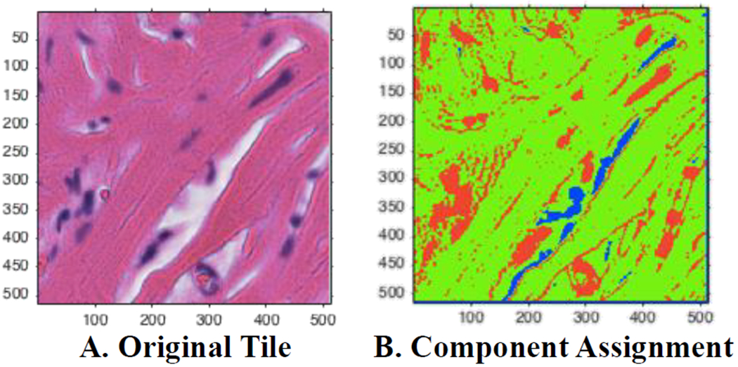
Two empty tile checks were embedded in this step. First, the standard deviation was calculated for each color channel in the RGB color space. If the standard deviation in each channel did not exceed a proposed threshold, the tile was excluded from further processing steps. The second check came after each pixel was assigned to a Gaussian Mixture Model component (Figure 2). If there were no pixels assigned to the pink/eosin group, the tile was considered empty of tissue samples and did not undergo further color normalization steps as was excluded from the rest of the overall pipeline. These steps were created under the assumption that tiles including tissue samples should have variation in the color distribution in the tile (unlike tiles of empty space on each slide between tissue samples) and should have at least one pixel assigned to the pink/eosin component as non-nuclear cell components are more prevalent than nucleic components that would be assigned to the purple/hematoxylin component.

Fig. 2:

Visualization of automated Gaussian mixture model assignments. (A) A sample tile with H&E staining. (B) Assigned pixels based on posterior probabilities. Green corresponds to the eosin/pink component, red assigned to the hematoxylin/purple, and blue corresponds to the background/white component.

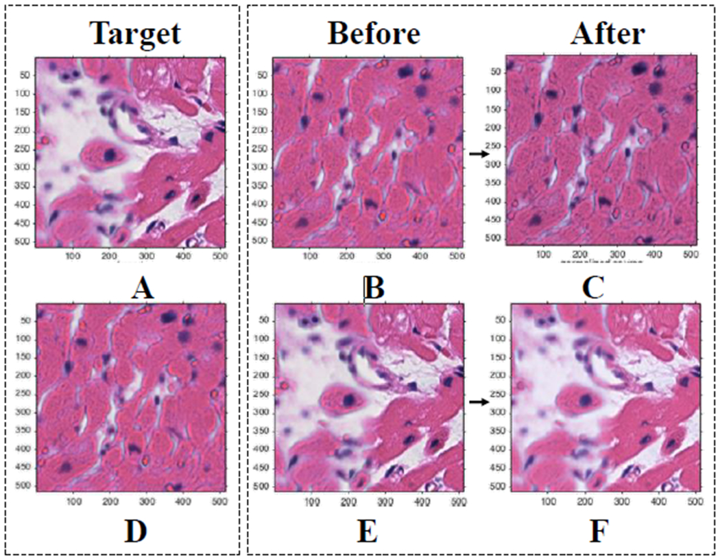
A Gaussian Mixture Model was used to assign each pixel (observation) to a component that maximized the component’s posterior probability. All tiles were converted to the CIE 1976 L*a*b* color space first, allowing for better segmentation using color channel thresholding. Reinhard’s method was applied to the pixels in each component separately. This involved converting the reference images and test image from RBG to XYZ to LMS to l-alpha-beta color space and calculating a linear transformation in each channel for each component [9]. Finally, each tile was converted back to RGB color-space following Reinhard’s linear transformation (Figure 4).

Fig. 4:

Results of color normalization step. (A) (D) Target images for (B) and (E) respectively. (B) (E) Original images. (C) (F) Mapped/normalized images. Demonstrates that proposed methods result in similar normalized pictures regardless of the amount of background in the target image.

A second empty tile check was applied through this step. Tiles were considered empty, and did not undergo the color normalization step, if there were no pixels assigned to the eosin/pink group. This step assumed that any slide with any amount of tissue sample should have some pixels assigned to the eosin/pink component.

C. Pixel-level Feature Extraction

Feature extraction can be used to gain more information about an image, such as color intensity and texture. Pixel level features extracted were based on Haralick features taken from gray-level-co-occurrence (GLCM) matrix and image histogram statistics. GLCMs were calculated for 1, 3, and 5-pixel wide neighborhoods at 0, 45, 90, and 135 degree angles [11]. These features help to describe the texture of each image by considering the relationship between the tone and texture, specifically the spatial distribution of the varying gray levels [12]. Image histogram statistics were taken in each of the three channels in three color spaces: RGB, HSV, and CIELAB spaces.

D. Object-level Feature Extraction

Object-level features are based on the known pathology of the different types of cardiac allograft rejection. Features that clinicians look for when classifying endomyocardial biopsy samples include dense mononuclear inflammatory infiltrates and the locations of those infiltrates [1]. The number of foci of infiltrate can also help distinguish between the classes and grading of rejection.

To relate pathological traits of rejection to the digitized whole slide images, we used color thresholding to map nuclei in each tile based on hematoxylin staining nuclear structures purple or blue. We created a binary image for each tile to capture nuclei as objects using color and size thresholding. Finally, we extracted features related to the size, density, and relative location of nuclei in each tile.

E. Principal Component Analysis

Principal component analysis was used as a tool for data visualization. The features that contribute the most to the first two principal components were ranked (Table I).

TABLE I:

Top 10 Features

Feature	Description	Type
dist_Mean	Average distance between objects	Object-level
area_Mean	Average size of object	Object-level
avg_L	Average value Channel 2 CIELAB	Pixel-level
perim_Mean	Average perimeter of object	Object-level
std_red	Standard Deviation Channel 1 RGB	Pixel-level
num_Mean	Average number of objects	Object-level
std-L	Standard Deviation Channel 1 CIELAB	Pixel-level
std_G	Standard Deviation Channel 2 RGB	Pixel-level
std_B	Standard Deviation Channel 3 RGB	Pixel-level
majAx_Mean	Average object major axis length	Object-level

F. Clustering

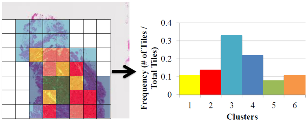
As each individual tile did not have a label, we used K-means clustering to group tiles. We used a squared Euclidean distance metric and six clusters (based on the Davies Bouldin criterion [13]). The main reason to include this step was to identify rare events, such as only a few tiles show signs of rejection, and incorporate multiple instance learning. At the end of this step, each WSI was represented as a normalized 1×6 vector with each entry representing the percentage of tiles of the WSI assigned that cluster (Figure 5). This newly created feature vector was used in the classification step instead of the original 129 feature vector.

Fig. 5:

Representation of clustering method with each tile of the WSI assigned to a cluster with the corresponding histogram.

G. Classification

A baseline was created by creating a feature distribution frequency for each slide following feature extraction. We used ten bins for each of the 129 features, as opposed to taking the mean or another metric, as the exact distribution of features was unknown. A vector of 1,290 elements was then created for each WSI.

Multiple machine learning algorithms were used for binary classification and prediction including decision trees (with 4, 20, and 100 maximum splits), logistic regression, linear and quadratic support vector machines (SVM), fine and course Gaussian SVM, k-nearest neighbors (1, 10, and 100 neighbors), boosted trees, and bagged trees. 5 fold cross-validation was used for each classification method.

III. RESULTS

For the baseline group, only logistic regression and linear SVM resulted in accuracy rates greater at or greater than 50%, with both accuracy rates at 50.0%. After clustering the features, linear SVM resulted in the highest accuracy score, 70.0%. Medium, cubic, and weighted KNN, as well as bagged trees, resulted in an accuracy rate of 66.7%.

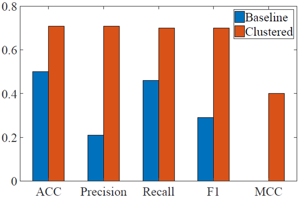
Focusing on the linear SVM algorithm for both the baseline and clustered data, binary classification metrics were calculated, including accuracy (ACC), precision, recall, factor 1 score (F1), and Matthews correlation coefficient (MCC) (Figure 6). The area under the receiver operating characteristic (ROC) curve for linear SVM following clustering was 0.67 and the area under the ROC curve for linear SVM without clustering was 0.39.

Fig. 6:

Classification accuracy metrics for linear SVM before and after clustering.

IV. CONCLUSIONS AND DISCUSSIONS

A major limitation of this study was the small sample size. Dividing each observational group into training and testing sets further reduced the number of observations that could train each classification model. Future revisions to this study should include adding more whole-slide images. This could help improve accuracy as well as allow for multi-class classification into types of rejection, ACR and AMR, as well as the grading schemes for rejection (0R, 1R, 2R, and 3R). We can also use hyperparameter tuning for the classification methods in future studies.

More features can also be extracted at both the pixel and object-level. Features that have been extracted in other studies using computer-aided diagnosis for histopathological features include Gabor and wavelet filters and topology features [4]. As most of the top ten contributing factors for PCA came from object-level features, looking into extracting more object-level features may improve overall predictive accuracy.

Also, more features that specifically describe the different types and grades of rejection, such as percent of monocyte inflammation and the locations of foci of infiltrates, can be extracted. This will be especially useful for multi-class classification, for distinguishing between ACR and AMR and different grades of rejection. This can include extracting a few features to describe a specific pathologic finding, such as the breakdown of the myocardium stratification or circular nuclei patterns around capillaries. These pathologic findings can then be combined, so that if more than one instance of specific features pathologists look for are present, the WSI cannot be classified as normal. A mask indicating regions of interests can also be developed to indicate areas that need to be further examined.

REFERENCES

- [1].Tan CD, Baldwin WM III, and Rodriguez ER, “Update on cardiac transplantation pathology,” Archives of pathology & laboratory medicine, vol. 131, no. 8, pp. 1169–1191, 2007. [DOI] [PubMed] [Google Scholar]
- [2].Costanzo MR, Dipchand A, Starling R, Anderson A, Chan M, Desai S, Fedson S, Fisher P, Gonzales-Stawinski G, Martinelli L, et al. “The international society of heart and lung transplantation guidelines for the care of heart transplant recipients,” 2010. [DOI] [PubMed]
- [3].Tong L, Hoffman R, Deshpande SR, and Wang MD, “Predicting heart rejection using histopathological whole-slide imaging and deep neural network with dropout,” in Biomedical & Health Informatics (BHI), 2017 IEEE EMBS International Conference on IEEE, 2017, pp. 1–4. [DOI] [PMC free article] [PubMed] [Google Scholar]
- [4].Kothari S, Phan JH, Stokes TH, and Wang MD, “Pathology imaging informatics for quantitative analysis of whole-slide images,” Journal of the American Medical Informatics Association, vol. 20, no. 6, pp. 1099–1108, 2013. [DOI] [PMC free article] [PubMed] [Google Scholar]
- [5].Barker J, Hoogi A, Depeursinge A, and Rubin DL, “Automated classification of brain tumor type in whole-slide digital pathology images using local representative tiles,” Medical image analysis, vol. 30, pp. 60–71, 2016. [DOI] [PubMed] [Google Scholar]
- [6].Fernández-Carrobles MM, Serrano I, Bueno G, and Déniz O, “Bagging tree classifier and texture features for tumor identification in histological images,” Procedia Computer Science, vol. 90, pp. 99–106, 2016. [Google Scholar]
- [7].Sertel O, Kong J, Shimada H, Catalyurek U, Saltz JH, and Gurcan MN, “Computer-aided prognosis of neuroblastoma on whole-slide images: Classification of stromal development,” Pattern recognition, vol. 42, no. 6, pp. 1093–1103, 2009. [DOI] [PMC free article] [PubMed] [Google Scholar]
- [8].Hoffman RA, Kothari S, and Wang MD, “Comparison of normalization algorithms for cross-batch color segmentation of histopathological images,” in Engineering in Medicine and Biology Society (EMBC), 2014 36th Annual International Conference of the IEEE IEEE, 2014, pp. 194–197. [DOI] [PMC free article] [PubMed] [Google Scholar]
- [9].Magee D, Treanor D, Crellin D, Shires M, Smith K, Mohee K, and Quirke P, “Colour normalisation in digital histopathology images,” in Proc Optical Tissue Image analysis in Microscopy, Histopathology and Endoscopy (MICCAI Workshop), vol. 100 Daniel Elson, 2009. [Google Scholar]
- [10].Reinhard E and Pouli T, “Colour spaces for colour transfer” in CCIW. Springer, 2011, pp. 1–15. [Google Scholar]
- [11].Zayed N and Elnemr HA, “Statistical analysis of haralick texture features to discriminate lung abnormalities,” Journal of Biomedical Imaging, vol. 2015, p. 12, 2015. [DOI] [PMC free article] [PubMed] [Google Scholar]
- [12].Haralick RM, Shanmugam K, et al. “Textural features for image classification,” IEEE Transactions on systems, man, and cybernetics, no. 6, pp. 610–621, 1973. [Google Scholar]
- [13].Liu Y, Li Z, Xiong H, Gao X, and Wu J, “Understanding of internal clustering validation measures,” in Data Mining (ICDM), 2010 IEEE 10th International Conference on IEEE, 2010, pp. 911–916. [Google Scholar]