Determining Free-Energy Differences Through Variationally Derived Intermediates

Abstract

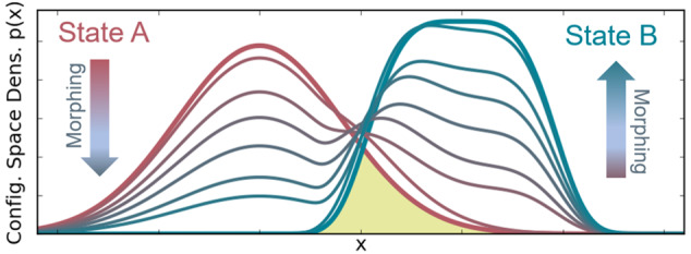
Free-energy calculations based on atomistic Hamiltonians and sampling are key to a first-principles understanding of biomolecular processes, material properties, and macromolecular chemistry. Here, we generalize the free-energy perturbation method and derive nonlinear Hamiltonian transformation sequences yielding free-energy estimates with minimal mean squared error with respect to the exact values. Our variational approach applies to finite sampling and holds for any finite number of intermediate states. We show that our sequences are also optimal for the Bennett acceptance ratio (BAR) method, thereby generalizing BAR to small sampling sizes and non-Gaussian error distributions.

1. Introduction

Free-energy calculations provide essential insights into numerous physical and biochemical systems. Examples range from predicting binding processes of biomolecules for drug design¹⁻³ to determining thermodynamic properties of crystalline materials.^4,5 For large and complex systems with slow relaxation rates and typically 10⁵ to 10⁷ particles, only limited accuracy is achieved,⁶ despite substantial methodological progress⁷⁻¹⁰ and immense computational effort. In addition to force field inaccuracies, insufficient sampling is the main bottleneck.¹¹ Within a generalized framework connecting two of the most established methods, free-energy perturbation (FEP)¹² and the Bennett acceptance ratio method (BAR),¹³ with the latter generally considered the more accurate one,¹⁴ we here will develop and evaluate a variational approach for optimal sampling that minimizes the error due to limited sampling.

Given the Hamiltonians H₁(x) and H_N(x) of two states 1 and N, where x ∈ ^3M denotes the position of all M particles of the simulation system, the free-energy difference ΔG_1,N between these states is given by the Zwanzig formula¹²

1

where ⟨⟩₁ denotes an ensemble average defined by H₁(x), which is approximated by averaging over a finite sample of size n obtained from atomistic simulations or Monte Carlo sampling. For ease of notation, all energies are expressed in units of k_BT.

Alchemical transformations substantially reduce errors in the free-energy estimates^15,16 by introducing N – 2 intermediate states s and accumulating small free-energy differences between all adjacent states s and s + 1,

2

Using the Zwanzig formula between s and s + 1, this technique is referred to as FEP. The same approach is also employed in other fields, for example in the context of Bayesian statistics, where the plausibility of two different models is compared by calculating their marginal likelihood ratio.^17,18

The most common interpolation scheme for the intermediate states is along a path variable λ.

3

Figure 1(a) shows, as a simple example, a linear interpolation between two one-dimensional Hamiltonians H₁(x) and H_N=9(x). In the case of soft-core potentials,¹⁹⁻²¹ a nonlinear dependence of the end states H₁(x, λ) and H_N(x, λ) on λ is introduced under the requirement that H₁(x, λ = 0) = H₁(x) and H_N(x, λ = 1) = H_N(x). In this context, finding better sequences of Hamiltonians by optimizing the distribution of λ points for a given form of a sequence or pathway has been attempted.²²

Figure 1.

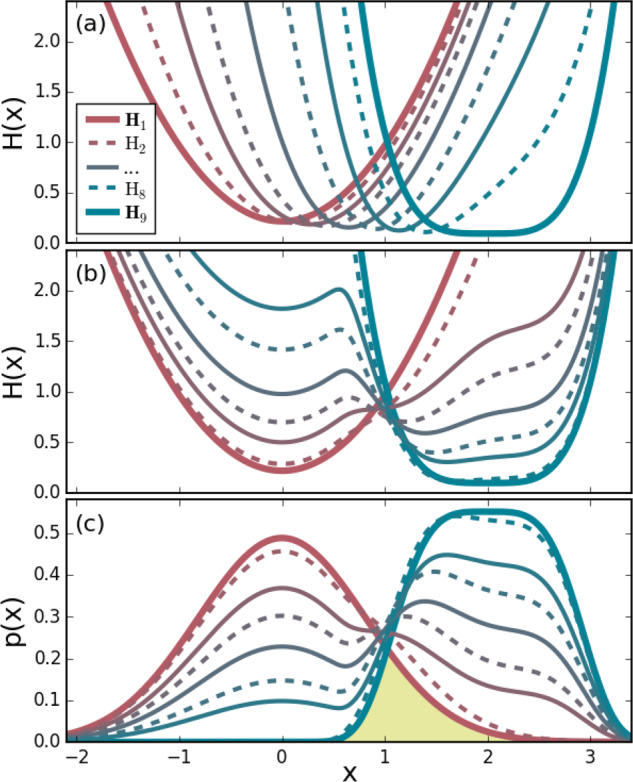
Sequences of intermediates between a harmonic potential and a quartic potential H₉(x) = (x – x₀)⁴ + c (thick lines), where b and c have been determined such that Z₁ = Z₉ = 1, i.e., ΔG_1,9 = 0. Sampling states are described by odd-numbered Hamiltonians (solid lines) and virtual target states by even-numbered ones (dashed lines). (a) A linear interpolation between H₁(x) and H₉(x). For better visualization, the intermediates are vertically offset to align the minima. (b) Intermediate Hamiltonians and (c) resulting configuration space densities of VI. The yellow area highlights the configuration space density overlap K between states 1 and 9.

Even though there is some freedom in the construction of these transformation sequences, eq 3 describes only a very small subset of all possible sequences of intermediate states and, in this sense, is not the most general. Specifically, the terms containing the information and parameters of the two different end states are always combined in an additive manner, and for example, any definition of intermediate Hamiltonians H_s(x) that would involve cross terms of the form f(H₁(x, λ) · H_N(x, λ)) would not be possible with the definition of eq 3.

Therefore, a number of alternative approaches that modify eq 3 have been developed. For example, an empirical potential has been proposed in the enveloping distribution sampling (EDS) method^23,24 that interpolates between the configuration space densities (rather than the Hamiltonians) of two or several end states and is, as we will find, remarkably close to the optimal solution for a single intermediate state.

Furthermore, a continuous path between two such end states, which optimizes the variance for thermodynamic integration (TI),²⁵ i.e., the minimum variance path (MVP), was first derived by Blondel,²⁶ and later through a different formalism by Pham and Shirts,²⁷ based on the results from the statistical sciences by Gelman and Meng.¹⁷

Here, we will generalize this interpolation scheme for FEP and BAR. Specifically, we ask which sequence H₂(x)... H_N–1(x), among all possible sequences of higher order functions {H_s[H₁(x), H_N(x)]} that map two functions onto functions H_s (with s = 2, ..., N – 1), yields on average the smallest mean squared error (MSE)

4

of the free-energy estimate ΔG⁽ⁿ⁾ obtained through finite sampling with n sample points with respect to the exact free-energy difference ΔG. Figure 1(b) and (c) show such a general interpolation sequence, which we refer to as the variationally derived intermediates (VI) method.

Our approach differs from previous approaches in that here we optimize the full MSE. Because the MSE can be decomposed into the sum of variance, [([ΔG⁽ⁿ⁾] – ΔG⁽ⁿ⁾)²], and squared bias, ([ΔG – ΔG⁽ⁿ⁾])², analyzing and optimizing these two terms separately has been attempted.^14,27−29 For the MVP in the context of TI, continuous sampling along the path variable λ is assumed; for practical applications, however, discrete integration is preferred, which implies an additional bias that is difficult to assess and, therefore, not included within the optimization. As we will find, optimizing the sum of both variance and bias yields a conceptually improved result.

2. Theory

2.1. Optimal Mean Squared Error Sequence of Intermediates for Free-Energy Perturbation

To solve the above variational problem and to find the optimal sequence of H_s, we consider the FEP scheme displayed in Figure 2(a) as one of several possible implementations of eq 2 using eq 1. In this particular variant, which is symmetric with respect to the exchange of the two end states to avoid hysteresis effects, sample points are solely drawn from the odd-numbered sampling states, indicated by the solid lines in Figures 1 and 2. The even-numbered states serve as virtual target states (dashed lines), similar to, for example, the overlap sampling method.³⁰ From the sum of the individual perturbation steps, the average MSE of this scheme is

5

As in Figure 2, the arrows point from sampling to target states.

Figure 2.

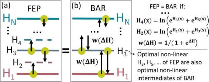
Two schemes of free-energy calculation. Yellow dots represent sample sets in the respective potential; arrows indicate the evaluation of differences ΔH(x) between adjacent Hamiltonians. Free-energy differences are either determined by (a) FEP or by (b) BAR with multiple steps. Both schemes give identical results at the stated conditions.

Assuming for each sample state s a set of n independent sample points {x_i}, drawn from , with partition function Z_s, the terms arising from expanding eq 5 will be considered one by one.

6

Because the exact free-energy difference is a constant,

7

For the linear term, the average over all sample realizations reads

8

and for the quadratic term

9

Similar expressions are obtained for ΔG_s+2→s+1⁽ⁿ⁾. The exact free-energy differences are

10

For shifted Hamiltonians H_s^′(x) = H_s(x) – C_s and H_s+1(x) = H_s+1(x) – C_s+1, eq 1 yields

11

which also holds for the exact value ΔG_1′,N′. The offsets on the right-hand side of eq 11 cancel out when calculating the MSE of eq 5. By choosing C_s and C_s+1 such that the term in the logarithm of eqs 8 and 9 is close to one, and thus all ΔG_{s′→(s+1)′}⁽ⁿ⁾ values are small with respect to k_BT = 1, the first order expansion of the logarithm allows the integrals to be factorized. Therefore

12

For the shifted Hamiltonians, the same expansion can be applied to the exact free-energy difference of eq 10. Therefore, eq 12 reduces to

13

The configuration space densities of the shifted and the initial Hamiltonians are identical; in other words

14

Note that the underlying assumption that the same offsets C_s and C_s+1 can be used to enable the series expansion of the exact and estimated free-energy differences. This assumption, as we will later find, holds for the vast majority of cases but may break down in the case of very few sample points and very low-configuration space density overlap between the two neighboring states.

For the cross terms in eq 6, note that the estimated free-energy differences of the individual steps are based on uncorrelated sample sets. Therefore

15

for (s′ → t′) ≠ (u′ → v′). Expanding eq 9 yields

16

Using eq 15, all expressions from the cross terms only depend on exact free-energy differences. By summarizing these terms by f_s′, eq 16 can be written as

17

Inserting eqs 13 and 17 into eq 5 gives the following:

18

where g_s′ again denotes an expression that only depends on exact free-energy differences and thus is dropped for the optimization below.

3. Results and Discussion

3.1. Optimal Sequence

With these expressions, the variational problem can be solved analytically. For the odd-numbered states s, the variation of the MSE(ΔG_1,N⁽ⁿ⁾) from eq 18 is

19

which yields

20

where Z_s = ∫ e^–H_s(x) dx is the (finite) partition sum and ν is a Lagrange multiplier.

Similarly, for the even-numbered states

21

An additive term C_s in eqs 20 and 21 was omitted, as it cancels in ΔG_s–1→s⁽ⁿ⁾ – ΔG_s+1→s. The result is a set of equations for all states s for which each Hamiltonian H_s(x) depends only on the two adjacent states. The initial requirement for small ΔG_{s′→(s+1)′}⁽ⁿ⁾ is fulfilled by setting C_s = −ln Z_s because, in this case, all Z_s′ are 1. Rearranging the terms for odd-numbered s gives

22

For the virtual target states (i.e., even-numbereds), rearranging yields

23

with r_s,t = Z_s/Z_t.

Equations 22 and 23 are the first main result of this article; they define the sequence of Hamiltonians yielding the best MSE for FEP free-energy calculations.

3.2. Generalization of BAR

The second main result is that eq 21 serves to generalize the BAR formula. To see this, consider eq 21 for N = 3, i.e., with one intermediate target state. Applied to the two involved free-energy differences, the Zwanzig formula yields

24

25

Inserting eq 21 as the target state Hamiltonian H₂(x) yields the BAR formula

26

with C = C₃ – C₁.

Notably, the above derivation yields the more general result that eq 26 also provides the best MSE free-energy estimate for finite and small n, even down to n = 1, given sufficient configuration space density overlap between adjacent states, which is fulfilled, for instance, in the limit of many intermediates. In contrast, because the derivation by Bennett¹³ strictly holds only for infinite sampling, so far, n was required to be large, and proper convergence had to be assumed. Furthermore, in the original derivation,¹³ the error distribution of the free-energy estimates had to be assumed to be Gaussian, which in our above result is also not required. While it has been known that BAR yields the lowest variance out of the asymptotically unbiased estimators,³¹ the above derivation shows that this also holds for the MSE at finite n and that BAR is the best out of all estimators, including, in addition, the asymptotically biased ones. In the context of the overlap sampling method,^{15,16,30,32,33} it has been shown that a virtual FEP intermediate can be defined that yields the weighting function from Bennett’s derivation; the above results prove that this intermediate is indeed optimal for the FEP scheme. Note that, in the extreme case of small configuration space density overlap and very few sample points, the average deviation between the series expansions of the exact and the estimated expressions of eq 12 can become too large, in which case our approach may miss the absolute optimum, and therefore, a better solution may exist. However, as we will see later in the context of Figure 6, the VI result yields a better MSE than all other approaches that we assessed, even for small n at small configuration space density overlaps between the end states.

Figure 6.

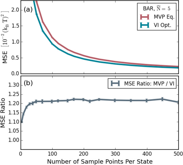
Comparison of the achieved accuracy by the minimum variance path method (MVP) and VI for different numbers of sample points per state using 5 states. (a) Obtained MSE for both methods and (b) their respective ratios.

The third main result is that the optimal intermediates for FEP are also optimal for BAR. To see this, consider again eqs 22 and 23, which optimal FEP intermediates for any (odd) number N – 2 of intermediate states. As was shown in the derivation of eq 26, using the intermediate of eq 23 with FEP between two sampling states is equivalent to using BAR between these two. Applied recursively to many states, and as illustrated in Figure 2, the Ñ = (N + 1)/2 sampling states from any sequence of N FEP-optimal Hamiltonians {H_s(x)} are also optimal for BAR with multiple states, where, so far, states have mostly been used in the form described in eq 3. The governing system of equations for BAR with multiple states is obtained by replacing H_s–1(x) and H_s+1(x) in eq 22 with the expression of eq 23, which for odd s yields

27

Here, the sampling states are now coupled directly, and only knowledge of the partition sum ratios between these is required. Solving the system of equations of eq 27 for all sampling states yields the intermediates with optimal MSE for BAR. Conversely, for the setup of one sampling state between two given target end states 1 and 3, eq 20 recovers the EDS potential when using a factor of 2 in the exponent of ref (24). In summary, both BAR and EDS are special cases of, or approximations to, our more general variational VI result that also requires fewer assumptions.

To solve eqs 22 and 23 for the optimal FEP intermediate Hamiltonians H_s(x), or alternatively eq 27, to directly obtain the optimal BAR intermediates, respectively, note that the unknown free-energy differences ΔG_s,t = −ln r_s,t are part of the equations that, therefore, have to be solved iteratively. With an initial guess for all r_s,t, the set of equations is solved in a point-wise fashion for any given x. After sampling all odd-numbered states, the r_s,t values are updated iteratively such that the sequence of intermediate states converges toward the optimum. This iteration converges to the optimal result because both the estimates as well as the linear approximation of the series expansion in eq 12 converge simultaneously. For a typical biomolecular many-body system, the additional computational effort is small compared to computing H₁(x) and H_N(x).

For the above illustrative example, Figure 1(b) and (c) shows the optimized Hamiltonians and the configuration space densities, respectively, of the converged sequence of intermediate states. To this end, initial values of r_s,t = 1 were used, and eqs 22 and 23 were iterated until convergence, using numerical integration over x and updating the r_s,t value during the process. Unlike the linear interpolations shown in Figure 1(a), the VI sequence leads to a probability density that gradually decreases in the region of A and increases in the region of B, while remaining almost constant at the point of maximum configuration space overlap.

3.3. One-Dimensional Test Case

Figure 3(a) shows the results of numerical simulations using the one-dimensional test case shown in Figure 1. Different equilibrium constants x₀ (42 different values) are used for H_N(x), thereby varying the configuration space overlaps between the end states, indicated by the yellow area in Figure 1(b).

28

Sets of n = 100 uncorrelated sample points are drawn from p_s(x) through rejection sampling in each of the Ñ = 3 sampling states. On the basis of these sets, BAR (solid lines) is used to calculate the free-energy difference between the individual states and subsequently between the start and end state. As a comparison, the dashed lines in Figure 1(a) show the results using MBAR,³¹ where the differences in the Hamiltonians for all states are considered for each sample point. The free-energy estimate is compared to the exact free-energy difference. For each K, the MSE, eq 5, is calculated by averaging over 600000 of such realizations.

Figure 3.

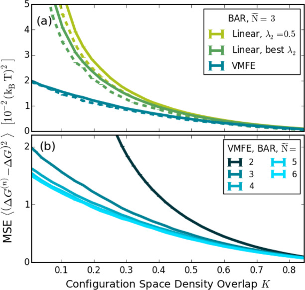
MSEs of free-energy calculations for different overlaps between the end states, determined numerically for the model Hamiltonians from Figure 1. For the solid lines, BAR is used between adjacent sampling states; for the dashed lines, MBAR is used. (a) Comparison between VI and two variants of linear intermediates: a linearly spaced λ₂ and an empirically optimized λ₂ yielding the lowest MSE. (b) Accuracies for different numbers of VI sampling states for a given total sampling size.

VI (blue curve) yields the smallest MSD for all K, compared to both the first linear interpolation variant (light green) using a linearly spaced , such as in a typical free-energy calculation, and even compared to the second variant (dark green) using the empirically determined λ₂ value that yields the best MSE that can be achieved by linear interpolation. To obtain the latter, we loop over the allowed range between zero and one in steps of 0.01. To reliably calculate the MSD with respect to the exact value, for each λ₂, 150000 free-energy estimates are calculated. Once the lowest MSE λ₂ value is determined, the corresponding MSD is calculated once again using 600000 realizations. The procedure is repeated for each value of K. We note that the λ₂ value yielding the best MSE varies for different K values and is inaccessible in practice for high-dimensional systems.

The largest improvements of VI are seen for small configuration space density overlaps that notoriously cause the largest uncertainties. Also for MBAR,³¹ shown by the dashed lines in Figure 3(a), VI gives the better MSE than the linear intermediates. Figure 3(b) shows how the MSE of VI improves with increasing numbers of states Ñ, keeping the total number of sample points, and hence the total computational effort, constant. For this example, the MSE increases up to Ñ = 5, beyond which no further improvement appears.

3.4. Approximated Sequence and Comparisons

In the above VI scheme, eqs 22 and 23 connect all intermediates and, therefore, cannot be solved efficiently in a straightforward way for many-particle systems. To overcome this limitation, we propose and assess two approximations that will yield analytical expressions for H_s, which can be used even in large-scale simulations. The first approximation is to switch to a hierarchical solution for the VI scheme. In a first step, the sampling state in the middle of the sequence, Ĥ_Ñ/2, is determined as the optimal state between H₁ and H_Ñ using eq 22. In the next step, Ĥ_Ñ/4 is determined as the optimal state between H₁ and Ĥ_Ñ/2, Ĥ_3Ñ/4 between Ĥ_Ñ/2 and H_Ñ, and so on. The hat above the Hamiltonian indicates the approximated form.

The second approximation is that only the sampling states are coupled using eq 22, and no virtual states are used. Therefore, while still using BAR between two adjacent sampling states, the states are optimized as if the Zwanzig formula, i.e., eq 1, was used to calculate the free-energy difference between them.

Using these two approximations, an analytical result for the sequence of intermediate states is obtained

29

where all Ĥ_s(x) are a function of only H₁ and H_Ñ and ζ ≈ [0, 1], and only C = C_N – C₁ ≈ ΔG has to be determined iteratively. Consequently, no other prior knowledge of the differences between the individual states is required, and therefore, the sampling simulations for each state can be run in parallel without communication. Note that these two approximations introduce a parameter ζ_s, which is not part of the exact result, as shown in eqs 22 and 23, and here, it plays a similar role as the λ_s parameter in eq 3 for linear intermediates.

For the one-dimensional example in Figure 1(c), Figure 4 compares the configuration space densities p(x) of the approximate intermediate Hamiltonians Ĥ_s(x) (dashed lines) with those of the optimal H_s(x) (solid lines). As can be seen, the overall shape is similar.

Figure 4.

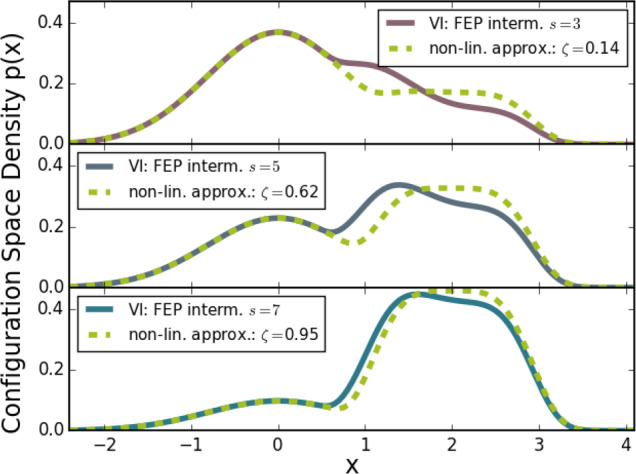
Comparison between configuration space densities of the approximated VI sequence, i.e., eq 29 (dashed lines), with that of the optimal VI sequence (solid lines) for the one-dimensional example shown in Figure 1(c). For better visualization, the three intermediate sampling states, s = 3, 5, 7, are shown separately.

The approximated VI in eq 29 is similar but not identical to the form of the MVP. The obvious difference to the approximated VI is the prefactor in the exponentials (2 and 1/2). The deeper conceptual difference, as outlined in the introduction, is that the approximated VI is an approximation to the sequence that optimizes the MSE and thereby also accounts for the biases. Furthermore, it is optimized for FEP and BAR, explicitly considering discrete states with finite sampling. In contrast, the MVP optimizes the variance for TI in the large sample limit by assuming independent samples, continuously drawn along the path variable λ.

Next, we compare both the optimal VI and the approximated VI to the MVP. Figure 5 shows the results for different numbers of intermediates states. The same model system and procedure as the one used to obtain the results for the comparison to the linear intermediates, shown in Figure 3 and described in section 3.3, is used. Again, for a fair comparison, the overall number of sample points was kept constant, i.e., the number of points per state is smaller for a larger number of intermediates.

Figure 5.

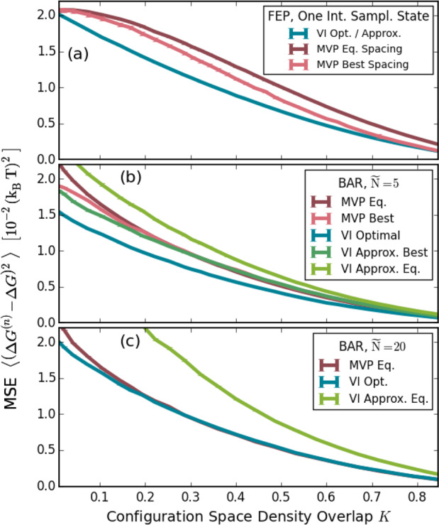
Comparison between the optimal VI, the approximated VI, and the MVP (minimum variance path)^26,27 at different numbers of sampling states Ñ. (a) One intermediate sampling state. FEP is used to determine the free-energy difference to the end states. In this case, the optimal VI equals the midpoint of the approximated VI. (b) Five sampling states. BAR is used to calculate the free-energy difference between these 5 states. The overall number of sample points is kept constant, i.e., the number of samples per state is lower for a higher number of states. (c) Using 20 sampling states, otherwise the underlying setup is identical to (b).

As can be seen, for all values of K, the optimal VI yields the smallest MSEs at all numbers of intermediates. The approximated VI, which is equivalent to the optimal VI at ζ = 0.5 when sampling in only one intermediate state (Figure 5(a)), therefore also yields a smaller MSE than both the midpoint MVP (λ = 0.5, purple) and the MVP with the best lambda (light red). The latter was again determined empirically by iterating over all possible lambda values in steps of 0.01.

Conversely, for 20 states, shown in Figure 5(c), the approximated VI yields a higher MSE, indicating that, for increasing numbers of steps, the approximations have a larger effect. Barring low values of K, similar MSEs are obtained for both the optimal VI and MVP because for large numbers of sampling states, FEP and TI become equivalent.

Interestingly, these MSEs are larger than for optimal VI with 5 states, shown in Figure 5(b), suggesting that there is an optimal number of states. Here, the MVP performs better than the approximated VI at equidistant spacing, whereas for the best spacing the respective MSEs are similar. For five states, the best spacing was obtained by adjusting the λ and ζ values such that the best fit of the configuration space densities with optimal VI was obtained, as shown in Figure 4. Through further variation, we tested if an even better combination of path variables could be found, which was not the case.

The fact that the approximated VI and the MVP converge to the optimal solution in opposite cases indicates that they are limiting cases to the general optimal VI result.

Figure 6 shows how the MSE depends on the number of sample points. The same procedure as for Figure 5(b) with five sampling states was used but now with only one equilibrium distance between the minima of the harmonic and quartic potential of x₀ = 3 (i.e., K ≈ 0.02, see Figure 1). To avoid the problem of the optimization of a path variable, we compare only the optimal VI and the MVP with equidistant spacing, which, in the case of Figure 5(b), yielded similar MSEs as the MVP with the best spacing.

As can be seen in panel (a), a smaller MSE is achieved by VI across a broad range of numbers of sample points. The ratio of the MSEs of both methods, Figure 6(b), is essentially constant, indicating an overall improvement of about 20–25%, which is independent of the sample size.

As discussed previously, both the variance and the bias contribute to the MSE. Surprisingly, we found that, for this setup, the bias is almost negligible, with the squared bias contributing less than 1% to the overall MSE for all n. Therefore, VI also yields a better variance than, despite what the name suggests, the minimum variance path by Blondel²⁶ and Pham and Shirts.²⁷ The reason is again that the latter was optimized under different assumptions and for a different estimator. However, note that while we have derived the sequence with the optimal MSE, the magnitude of the improvement compared to, for example, linearly interpolated intermediates is system dependent and, as we will see, actually can be much larger for many-particle systems than for one-dimensional ones.

4. Atomistic Test Cases

To compare the MSE of VI with that of established intermediates, we have performed test simulations for two atomistic many-particle simulation systems: a Lennard-Jones gas and a solvated butanol molecule.

4.1. Lennard-Jones Gas

The free-energy difference between an argon and a helium Lennard-Jones (LJ) gas with M = 20 atoms was calculated. A reference free-energy difference was determined by conducting a long simulation with each method using 12 states with linearly spaced λ_s values for both the linear intermediates and the approximated VI sequence and with computation runs of 10 μs in each state. At this length, the relative difference of the estimates between the two methods is below 10^–5 (ΔG = 0.23252k_BT). Using this reference value, the MSE with a distribution of 800 free-energy differences, determined with only five intermediates depending on the simulation time in each state, was calculated.

In each state, the atoms were placed at random positions without overlap inside a cubic box. The atoms were assigned velocities drawn from the Boltzmann distribution corresponding to the temperature of T = 298 K. The simulations were conducted in the NVT ensemble at T = 298 K in a cubic box using periodic boundary conditions. The volume of the box was set to (43.5 Å)³, corresponding to a pressure of about 10 bar. The atomic interaction at a distance r between the centers of two atoms was described through a Lennard-Jones potential:

30

with parameters σ = 3.405 Å, ϵ = 1.0446 kJ/mol and m = 39.95 u for argon and σ = 2.64 Å, ϵ = 0.0906 kJ/mol and m = 4 u for helium.³⁴

The leapfrog algorithm with a time step of 5 fs was used and with velocity rescaling at every 20th time step. For both sequences, the 800 free-energy simulations were carried out with 1 ns equilibration time and 5 ns production runs in each state. Five intermediate states, i.e., seven states in total, were used. In absence of further knowledge, equal spacing of λ_s and ζ_s, i.e, {0, 0.17, 0.33, 0.5, 0.67, 0.83, 1} was used. For the approximated VI sequence (eq 29), C = 0 was used throughout the whole simulation. The difference of the Hamiltonians between adjacent states was recorded at every 200th step. Free-energy differences were subsequently calculated using BAR.

Figure 7 shows the resulting MSEs. For short simulation lengths, the MSE improves rapidly. For longer simulation times, the improvement of VI becomes most pronounced. At 5 ns, VI (green) has a four times lower MSE than the conventional linear intermediates (red). Conversely, the MSE achieved by linear intermediates at 5 ns is already obtained at 0.56 ns by VI, which, at this level, thus requires almost 10 times less sampling.

Figure 7.

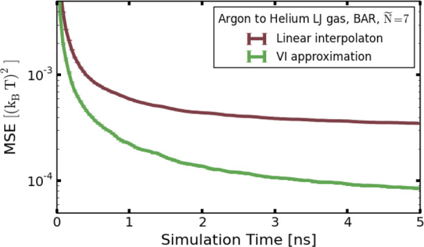
An argon LJ gas is morphed into a helium LJ gas. The MSE with respect to a converged reference value is shown as a function of the simulation time in each intermediate. It was obtained using linear intermediates (red) and the approximated VI intermediates (green). For both, an equal spacing of λ values and ζ values, respectively, has been used.

4.2. Charge Decoupling of Butanol

For a last system closer to biomolecular applications, the approximated VI intermediates were implemented into GROMACS 2019. We calculated the solvation free-energy difference between charged and uncharged butanol (15 atoms) solvated in water (1800 atoms in total). The topology from the SolvationToolkit package from Bannan et al.³⁵ was used. As for the Lennard-Jones gas, a reference value was obtained through extensive simulations, which then was compared to the estimates of a number of shorter simulations with fewer states. For the reference value, we used 51 linear intermediates with equidistant λ states (i.e., Δλ = 0.02) and production runs of 100 ns simulation time in each state, totalling 5.1 μs of simulation time. Energy values were recorded at every 200th step. Equilibration of 100 ps at constant volume and 200 ps at constant pressure with the Parrinello–Rahman barostat³⁶ was conducted prior to the production runs.

A reference value between the coupled and decoupled charges of 8.708 ± 0.001 k_BT was obtained. Next, simulations in five different states were carried out with both conventional linear intermediates and VI using λ_s and ζ_s values of 0, 0.25, 0.5, 0.75, and 1, respectively. In each state, five production runs were each conducted with 100 ns of simulation time, and smaller portions of the trajectories of different lengths were used to asses the MSEs as a function of the trajectory length. For each trajectory length, a free-energy difference estimate was calculated.

Figure 8 shows the obtained MSE for linear intermediates as well as for three different VI variants (see Supporting Information for a table of the MSEs), which differ in the choice of the initial guess. The MSE of the VI sequence with the exact estimate (blue) for C in eq 29 is about a factor of 2 better than the linear intermediates (red) at all simulation lengths, or equivalently, only half the amount of simulation time is necessary to obtain the same level of the MSE. For an unrealistically large error in the initial guess C, the MSE of the VI sequence is larger (green). However, with a more realistic initial estimate deviating by 1 k_BT from the reference value (yellow), the MSE also improved by about a factor of 2 with respect to the linear intermediates, barring very long simulation lengths. Such estimates can, for example, easily be obtained by linear intermediates with a simulation time of less than 40 ps, and therefore only a small fraction of the total simulation time, after which the VI becomes the significantly better option than linear intermediates. In addition, the estimate can be further refined during the simulation process.

Figure 8.

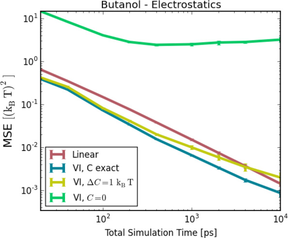
Accuracies of the estimates for the solvation free-energy difference between charged and uncharged butanol with respect to the simulation time. Linear intermediates (red) are compared to VI using different initial guesses.

5. Conclusions

Using a variational principle, we have derived a minimum MSE sequence of intermediate Hamiltonians for free-energy calculations using FEP and BAR. Our approach differs from previous ones in that it, first, optimizes the full MSE with respect to the exact free-energy difference rather than the variance only (i.e., the precision). Second, it directly optimizes the sequence of discrete states instead of a two step approach, where first a continuous TI path is optimized^17,26,27 and subsequently a discrete subset of states is chosen from this path. Third, it holds for finite sampling and for any number of intermediate states, thus proving analytically that BAR is also the optimal MSE estimator for finite sampling.

We assessed the performance of our method using three test systems. First, a simple one-dimensional model was considered. Compared to linear interpolations, a marked improvement in the MSEs was observed. Two limiting cases of our general VI result are notable. In the limit of many steps, the MSEs of the optimal VI and the MVP^17,26,27 are similar. In the limit of a few steps, an approximated sequence was derived, the form of which appears similar to MVP but differs in the exponent by factors of 2 and 1/2. However, for this model, the smallest overall MSE was achieved for a given computational effort at a medium number of intermediates (five in our case). Interestingly, the improvement in the MSE of the optimal VI compared to the MVP was mainly due to improvements of the variance; thus, the discretization of the path affects not only the bias but also the variance.

Next, we considered an argon and a helium LJ gas and, somewhat closer to real applications for complex biomolecular systems, the solvation free-energy difference between charged and uncharged butanol. For both many-particle test systems, marked improvements compared to conventional intermediates were seen.

This work focused on the theory and derivation of our variational approach. We have so far not tested our method on larger, more complex biomolecular systems involving conformational transitions. Therefore, further work is required toward the practical applicability, along several lines.

First, VI was derived assuming statistically independent sample points x_i. For atomistic simulation-based sampling and, to a lesser extent, MC sampling, subsequent sample points are typically correlated, however, particularly when the relevant configuration space densities are separated by large barriers. In these cases, VI is not necessarily the optimal sequence but can be combined with enhanced sampling techniques, such as Hamiltonian replica exchange,³⁷⁻³⁹ appropriate biasing potentials,⁴⁰⁻⁴² or a combination thereof. Another possible route, indicated by the EDS method,^23,24 is to change the Hamiltonians in order to reduce energy barriers and thereby reduce time-correlations. We are, however, unaware of any variational approach to optimize this trade-off, and therefore, further research will be required toward this aim.

Second, VI requires an initial estimate of the free-energy differences. For all of our test cases, this requirement involved only little additional computational cost. Whether this remains true for more complex biomolecular systems remains unclear at present.

Third, vanishing particles are a particular challenge due to possible singularities. Interestingly, preliminary simulations (data not shown) on systems with such vanishing LJ particles suggest that VI automatically generates intermediate Hamiltonians that resemble soft-core potentials. However, the singularities still caused instabilities in our test simulations. Smoothening the potential of the VI intermediates in these regions avoided this problem, suggesting that VI can also be used in this context. Clearly, additional work will be required to provide a widely applicable sequence for the disappearance of particles in solution.

Supporting Information Available

The Supporting Information is available free of charge at https://pubs.acs.org/doi/10.1021/acs.jctc.0c00106.

• Table of mean squared errors as a function of total simulation time for the electrostatic decoupling of solvated butanol (PDF)

The authors declare no competing financial interest.

References

- Williams-Noonan B. J.; Yuriev E.; Chalmers D. K. Free Energy Methods in Drug Design: Prospects of ”Alchemical Perturbation” in Medicinal Chemistry. J. Med. Chem. 2018, 61, 638–649. 10.1021/acs.jmedchem.7b00681. [DOI] [PubMed] [Google Scholar]
- Cournia Z.; Allen B.; Sherman W. Relative Binding Free Energy Calculations in Drug Discovery: Recent Advances and Practical Considerations. J. Chem. Inf. Model. 2017, 57, 2911–2937. 10.1021/acs.jcim.7b00564. [DOI] [PubMed] [Google Scholar]
- Christ C. D.; Fox T. Accuracy Assessment and Automation of Free Energy Calculations for Drug Design. J. Chem. Inf. Model. 2014, 54, 108–120. 10.1021/ci4004199. [DOI] [PubMed] [Google Scholar]
- Swinburne T. D.; Marinica M.-C. Unsupervised Calculation of Free Energy Barriers in Large Crystalline Systems. Phys. Rev. Lett. 2018, 120, 135503. 10.1103/PhysRevLett.120.135503. [DOI] [PubMed] [Google Scholar]
- de Koning M.; Antonelli A.; Yip S. Optimized Free-Energy Evaluation Using a Single Reversible-Scaling Simulation. Phys. Rev. Lett. 1999, 83, 3973–3977. 10.1103/PhysRevLett.83.3973. [DOI] [Google Scholar]
- Zuckerman D. M.; Woolf T. B. Theory of a Systematic Computational Error in Free Energy Differences. Phys. Rev. Lett. 2002, 89, 180602. 10.1103/PhysRevLett.89.180602. [DOI] [PubMed] [Google Scholar]
- Jarzynski C. Nonequilibrium Equality for Free Energy Differences. Phys. Rev. Lett. 1997, 78, 2690–2693. 10.1103/PhysRevLett.78.2690. [DOI] [Google Scholar]
- Vaikuntanathan S.; Jarzynski C. Escorted Free Energy Simulations: Improving Convergence by Reducing Dissipation. Phys. Rev. Lett. 2008, 100, 190601. 10.1103/PhysRevLett.100.190601. [DOI] [PubMed] [Google Scholar]
- Valsson O.; Parrinello M. Variational Approach to Enhanced Sampling and Free Energy Calculations. Phys. Rev. Lett. 2014, 113, 090601. 10.1103/PhysRevLett.113.090601. [DOI] [PubMed] [Google Scholar]
- Shirts M. R.; Bair E.; Hooker G.; Pande V. S. Equilibrium Free Energies from Nonequilibrium Measurements Using Maximum-Likelihood Methods. Phys. Rev. Lett. 2003, 91, 140601. 10.1103/PhysRevLett.91.140601. [DOI] [PubMed] [Google Scholar]
- Aldeghi M.; Gapsys V.; De Groot B. L. Accurate Estimation of Ligand Binding Affinity Changes upon Protein Mutation. ACS Cent. Sci. 2018, 4, 1708–1718. 10.1021/acscentsci.8b00717. [DOI] [PMC free article] [PubMed] [Google Scholar]
- Zwanzig R. W. High Temperature Equation of State by a Perturbation Method. I. Nonpolar Gases. J. Chem. Phys. 1954, 22, 1420–1426. 10.1063/1.1740409. [DOI] [Google Scholar]
- Bennett C. H. Efficient estimation of free energy differences from Monte Carlo data. J. Comput. Phys. 1976, 22, 245–268. 10.1016/0021-9991(76)90078-4. [DOI] [Google Scholar]
- Shirts M. R.; Pande V. S. Comparison of efficiency and bias of free energies computed by exponential averaging, the Bennett acceptance ratio, and thermodynamic integration. J. Chem. Phys. 2005, 122, 144107. 10.1063/1.1873592. [DOI] [PubMed] [Google Scholar]
- Lu N.; Kofke D. A. Accuracy of free-energy perturbation calculations in molecular simulation. I. Modeling. J. Chem. Phys. 2001, 114, 7303–7311. 10.1063/1.1359181. [DOI] [Google Scholar]
- Lu N.; Kofke D. A. Accuracy of free-energy perturbation calculations in molecular simulation. II. Heuristics. J. Chem. Phys. 2001, 115, 6866–6875. 10.1063/1.1405449. [DOI] [Google Scholar]
- Gelman A.; Meng X.-l. Simulating normalizing constants: from importance sampling to bridge sampling to path sampling. Statistical Science 1998, 13, 163–185. 10.1214/ss/1028905934. [DOI] [Google Scholar]
- Habeck M. Bayesian Estimation of Free Energies From Equilibrium Simulations. Phys. Rev. Lett. 2012, 109, 100601. 10.1103/PhysRevLett.109.100601. [DOI] [PubMed] [Google Scholar]
- Beutler T. C.; Mark A. E.; van Schaik R. C.; Gerber P. R.; van Gunsteren W. F. Avoiding singularities and numerical instabilities in free energy calculations based on molecular simulations. Chem. Phys. Lett. 1994, 222, 529–539. 10.1016/0009-2614(94)00397-1. [DOI] [Google Scholar]
- Zacharias M.; Straatsma T. P.; McCammon J. A. Separation-shifted scaling, a new scaling method for Lennard-Jones interactions in thermodynamic integration. J. Chem. Phys. 1994, 100, 9025–9031. 10.1063/1.466707. [DOI] [Google Scholar]
- Steinbrecher T.; Mobley D. L.; Case D. A. Nonlinear scaling schemes for Lennard-Jones interactions in free energy calculations. J. Chem. Phys. 2007, 127, 214108. 10.1063/1.2799191. [DOI] [PubMed] [Google Scholar]
- Shenfeld D. K.; Xu H.; Eastwood M. P.; Dror R. O.; Shaw D. E. Minimizing thermodynamic length to select intermediate states for free-energy calculations and replica-exchange simulations. Physical Review E 2009, 80, 049904. 10.1103/PhysRevE.80.049904. [DOI] [PubMed] [Google Scholar]
- Christ C. D.; van Gunsteren W. F. Enveloping distribution sampling: A method to calculate free energy differences from a single simulation. J. Chem. Phys. 2007, 126, 184110. 10.1063/1.2730508. [DOI] [PubMed] [Google Scholar]
- Christ C. D.; Van Gunsteren W. F. Multiple free energies from a single simulation: Extending enveloping distribution sampling to nonoverlapping phase-space distributions. J. Chem. Phys. 2008, 128, 174112. 10.1063/1.2913050. [DOI] [PubMed] [Google Scholar]
- Kirkwood J. G. Statistical Mechanics of Fluid Mixtures. J. Chem. Phys. 1935, 3, 300–313. 10.1063/1.1749657. [DOI] [Google Scholar]
- Blondel A. Ensemble variance in free energy calculations by thermodynamic integration: Theory, optimal ”Alchemical” path, and practical solutions. J. Comput. Chem. 2004, 25, 985–993. 10.1002/jcc.20025. [DOI] [PubMed] [Google Scholar]
- Pham T. T.; Shirts M. R. Optimal pairwise and non-pairwise alchemical pathways for free energy calculations of molecular transformation in solution phase. J. Chem. Phys. 2012, 136, 124120. 10.1063/1.3697833. [DOI] [PubMed] [Google Scholar]
- Gore J.; Ritort F.; Bustamante C. Bias and error in estimates of equilibrium free-energy differences from nonequilibrium measurements. Proc. Natl. Acad. Sci. U. S. A. 2003, 100, 12564–12569. 10.1073/pnas.1635159100. [DOI] [PMC free article] [PubMed] [Google Scholar]
- Oberhofer H.; Dellago C. Optimum bias for fast-switching free energy calculations. Comput. Phys. Commun. 2008, 179, 41–45. 10.1016/j.cpc.2008.01.017. [DOI] [Google Scholar]
- Lu N.; Kofke D. A.; Woolf T. B. Improving the efficiency and reliability of free energy perturbation calculations using overlap sampling methods. J. Comput. Chem. 2004, 25, 28–40. 10.1002/jcc.10369. [DOI] [PubMed] [Google Scholar]
- Shirts M. R.; Chodera J. D. Statistically optimal analysis of samples from multiple equilibrium states. J. Chem. Phys. 2008, 129, 124105. 10.1063/1.2978177. [DOI] [PMC free article] [PubMed] [Google Scholar]
- Lu N.; Wu D.; Woolf T. B.; Kofke D. A. Using overlap and funnel sampling to obtain accurate free energies from nonequilibrium work measurements. Phys. Rev. E 2004, 69, 057702. 10.1103/PhysRevE.69.057702. [DOI] [PubMed] [Google Scholar]
- Wu D.; Kofke D. A. Phase-space overlap measures. II. Design and implementation of staging methods for free-energy calculations. J. Chem. Phys. 2005, 123, 084109. 10.1063/1.2011391. [DOI] [PubMed] [Google Scholar]
- White J. A. Lennard-Jones as a model for argon and test of extended renormalization group calculations. J. Chem. Phys. 1999, 111, 9352–9356. 10.1063/1.479848. [DOI] [Google Scholar]
- Bannan C. C.; Calabró G.; Kyu D. Y.; Mobley D. L. Calculating Partition Coefficients of Small Molecules in Octanol/Water and Cyclohexane/Water. J. Chem. Theory Comput. 2016, 12, 4015–4024. 10.1021/acs.jctc.6b00449. [DOI] [PMC free article] [PubMed] [Google Scholar]
- Parrinello M.; Rahman A. Polymorphic transitions in single crystals: A new molecular dynamics method. J. Appl. Phys. 1981, 52, 7182–7190. 10.1063/1.328693. [DOI] [Google Scholar]
- Swendsen R. H.; Wang J.-S. Replica Monte Carlo Simulation of Spin-Glasses. Phys. Rev. Lett. 1986, 57, 2607–2609. 10.1103/PhysRevLett.57.2607. [DOI] [PubMed] [Google Scholar]
- Liu P.; Kim B.; Friesner R. A.; Berne B. J. Replica exchange with solute tempering: A method for sampling biological systems in explicit water. Proc. Natl. Acad. Sci. U. S. A. 2005, 102, 13749–13754. 10.1073/pnas.0506346102. [DOI] [PMC free article] [PubMed] [Google Scholar]
- Tan Z. Optimally Adjusted Mixture Sampling and Locally Weighted Histogram Analysis. Journal of Computational and Graphical Statistics 2017, 26, 54–65. 10.1080/10618600.2015.1113975. [DOI] [Google Scholar]
- Grubmüller H. Predicting slow structural transitions in macromolecular systems: Conformational flooding. Phys. Rev. E: Stat. Phys., Plasmas, Fluids, Relat. Interdiscip. Top. 1995, 52, 2893–2906. 10.1103/PhysRevE.52.2893. [DOI] [PubMed] [Google Scholar]
- Steiner M. M.; Genilloud P.-A.; Wilkins J. W. Simple bias potential for boosting molecular dynamics with the hyperdynamics scheme. Phys. Rev. B: Condens. Matter Mater. Phys. 1998, 57, 10236–10239. 10.1103/PhysRevB.57.10236. [DOI] [Google Scholar]
- Laio A.; Parrinello M. Escaping free-energy minima. Proc. Natl. Acad. Sci. U. S. A. 2002, 99, 12562–12566. 10.1073/pnas.202427399. [DOI] [PMC free article] [PubMed] [Google Scholar]
Associated Data
This section collects any data citations, data availability statements, or supplementary materials included in this article.