Radial Basis Function Approximation Optimal Shape Parameters Estimation

Abstract

Radial basis functions (RBF) are widely used in many areas especially for interpolation and approximation of scattered data, solution of ordinary and partial differential equations, etc. The RBF methods belong to meshless methods, which do not require tessellation of the data domain, i.e. using Delaunay triangulation, in general. The RBF meshless methods are independent of a dimensionality of the problem solved and they mostly lead to a solution of a linear system of equations. Generally, the approximation is formed using the principle of unity as a sum of weighed RBFs. These two classes of RBFs: global and local, mostly having a shape parameter determining the RBF behavior. In this contribution, we present preliminary results of the estimation of a vector of “optimal” shape parameters, which are different for each RBF used in the final formula for RBF approximation. The preliminary experimental results proved, that there are many local optima and if an iteration process is to be used, no guaranteed global optima are obtained. Therefore, an iterative process, e.g. used in partial differential equation solutions, might find a local optimum, which can be far from the global optima.

Introduction

Interpolation and approximation of acquired data is required in many areas. Usually a data domain is tessellated, i.e. meshed by triangles or tetrahedrons, using Delaunay tessellation [7]. However, there are some complications using this approach: Delaunay tessellation is not acceptable for some computational methods (other criteria for the shape of elements are required) and for computational and memory requirements in the case of higher dimensions. Also, if used for physical phenomena interpolation, there are additional problems with smoothness physical phenomena interpolation over resulting triangles or tetrahedrons. In the case of approximation, i.e. when the input data are to be reduced with regard to the values given, standard mesh reduction methods are complex as they are primarily designed for surface representation.

Meshless methods based on radial basis function (RBF) are based on the principle partition of unity, in general [2, 8, 28]. They are used for computations [1], e.g. partial differential equations (PDE) [6, 30, 31], interpolation and approximation of given data [16, 17], which lead to implicit representation [9, 18, 19] or explicit representation [10–12], impainting removal [25, 26, 29] vector data approximation (fluids, etc.) [24]. In the following, the RBFs for explicit representation will be explored more deeply from the shape parameter behavior and its estimation.

The RBFs interpolation is defined as [6, 20]:

1

where are coefficients and is a RBF kernel, and is an independent variable in -dimensional space, in general. If scalar values are given in points, i.e. , , then a system of linear equations is obtained

2

This leads to a system of linear equations . If and all points are distinct, then we have an interpolation scheme, if than the approximation scheme is obtained, as the system of equations is overdetermined [6, 10, 13, 20, 21, 27].

However, in our case we use the interpolation scheme, i.e. , and used only points of extrema, inflection points and some additional points, using the RBF interpolation scheme, to study estimation of a suboptimal selection of weights and shape parameters of the RBF interpolation. In this case, we obtain a system of linear equations:

3

The RBF interpolation was originally introduced as a multiquadric method by Hardy [5] in 1971. Since then, many different RFB interpolation schemes have been developed with some specific properties [3, 4].

The RBF kernel functions can be split to two main groups (just some examples):

• Global functions:

  • Gauss - ,
  • Multiquadric (MQ) - ,
  • Inverse multiquadric (IMQ) - ,
  • MQ-LG - [31]
  • Thin Spline (TPS)

    • ,
    • 

• Local - Compactly Supported RBF (CSRBF), e.g.

“+” means zero if a function argument is out of the interval.

Some of those are presented at Table 1 and Fig. 1.

Table 1.

Typical examples of “local” functions – CSRBF (“” means – value zero out of )

ID	Function	ID	Function
1		6
2		7
3		8
4		9
5		10

Fig. 1.

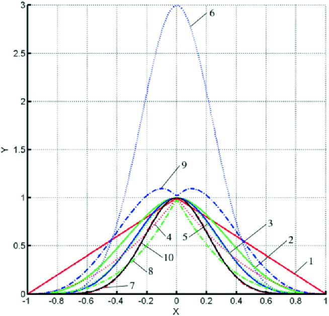
CS RBF functions

New RBF functions were recently introduced by Menandro [15].

They generally depend on a shape parameter, which must be carefully set up. Unfortunately, global functions lead to ill-conditioned systems, while CSRBF causes “blobby” behavior [23].

In this contribution, a slightly different problem is solved. Consider given points of an explicit curve; we aim to approximate it, strictly complying with the following requirements for the approximated curve and we want to approximate it having strict the following requirements for the approximated curve:

• it has to pass through all points of extreme and also points of inflection

• it keeps the value at the data interval border

Usually, the approximation case is solved using least square error (LSE) methods. The LSE application leads to good results in general, however, the LSE cannot guarantee the above-stated requirements. On the other hand, signal theory says that the sampling frequency should be two times higher than the highest frequency in the data. Also, different parts of a signal might have different high frequencies.

Therefore, the signal reconstruction should follow the local properties of the signal, if it would respect only the global properties, the compression ratio of the approximated signal would be lower and the sampling theorem is fulfilled. However, in practical experiments error behavior at the interval borders is to be improved by adding two additional points close to the border.

It means, that formally standard RBF interpolation scheme is obtained in which only points of extrema and inflection, points at the interval borders and two additional points are taken into account. Additional points only slightly improve interpolation precision.

However, the majority of RBFs depends on the “magic” constant – a shape parameter, which has a significant influence to the robustness, stability and precision of computation. Usually, some standard estimation formulas are used for the constant shape parameter, i.e. all RBFs have the same shape parameter. In the following, the case, when each kernel RBF has a non-constant parameter is described.

Determination of RBF Shape Parameters

Signal reconstruction using radial basis functions has to respect the basic requirements stated above. The sampling frequency should be locally two times higher than the highest frequency as the sampling theorem says. Therefore, if the values at the points of extrema and points of inflections are respected together with the values at the interval border, the sampling theory is fulfilled [14].

The question of choosing the shape parameters is not considered, yet. The global constant shape parameter, i.e. for all RBFs in the RBF approximation is to be used, the minimization process can be used

4

where for all , i.e. all shape parameters are the same.

However, if the shape parameters can differ from each other, the approximation will be more precise with fewer reference points, which also speed-up the RBF function evaluation. The question is, whether there is a unique optimum. Therefore, the “Monte-Carlo” approach was taken and the minimization process was initiated for different starting vector (uniformly generated using Halton’s distribution) of shape parameters using Gauss function.

5

It can be seen, that finding optimum shape parameter vector is computationally expensive. In the following, only one representative example from experiments made is presented.

Experimental Results

Several explicit functions have been used to understand the behavior of the optimal shape parameter vector determination (Table 2).

Table 2.

Examples of testing functions.

ID	Function	ID	Function
1		2
3		4
5		6
7		8
9		10
11		12
13		14
15		16

The experiments were implemented in MATLAB. The experiments proved, that there are several different shape parameters vectors, which give a local minimum of approximation error. In all cases, the error of the function values was less than , with a minimum number of points.

In the following, just two examples of RBF approximation are presented, additional examples can be found at [32]. Figure 2 presents two functions and their RBF approximation using found points of importance. Figure 3a presents shape parameters for each local optima found; the blue one is for a starting vector with an optimal global shape constant for all RBFs. Figure 3b presents computed weights of the RBF approximation.

Fig. 2.

Two examples of an approximated functions with approximation

Fig. 3.

Diagram of shape parameters vectors (a) and weights for local optima found (b)

The radial distances in the graphs are transformed monotonically, but nonlinearly to obtain “visually reasonable” graphs as:

It can be seen, that the shape parameters for each local optimum changes significantly, while the computed weights are similar. The experiments made on several explicit functions proved a hypothesis, that there are several local optima and for all of those a similar behavior was identified.

However, it leads to a serious question, how the RBFs use in the solution of ordinary and partial differential equations, in approximation and interpolation, etc. is a computationally reliable method, as results depend on “good” choice of the vector of shape parameters.

Detailed test results for several testing functions can be found at [32] http://wscg.zcu.cz/RBF-shape/contents-new.htm.

Conclusion

In this contribution, we shortly described preliminary experimental results in finding optimal shape vector parameters, i.e. when each RBF has a different shape parameter, which leads to the higher precision of approximation of the given data. The experiments were made on different explicit curves to prove basic properties of the approach. The experiments proved that there are several local optima for the shape vector parameters, which leads to different precision of the final approximation. However, it should be stated, that the approximation was made with relatively high compression and the error was lower than 10⁻⁵, which is in many cases acceptable. The given approach approximates data having different local frequencies will be explored in future together with an extension to explicit functions of two variables. The presented approach and results obtained should also have an influence to solution of partial differential equations (PDE), as the precision of a solution depends on good shape parameter selection.

The presented approach will be studied especially for the explicit functions of two variables, i.e. , where order is not defined and finding the nearest neighbors is too computationally expensive in the case of scattered data.

References

- 1.Biancolini, M.E.: Fast Radial Basis Functions for Engineering Applications. Springer Verlag (2017). 10.1007/978-3-319-75011-8
- 2.Buhmann MD. Radial Basis Functions: Theory and Implementations. Cambridge: Cambridge University Press; 2008. [Google Scholar]
- 3.Cervenka M, Smolik M, Skala V, et al. A new strategy for scattered data approximation using radial basis functions respecting points of inflection. In: Misra S, et al., editors. Computational Science and Its Applications – ICCSA 2019; Cham: Springer; 2019. pp. 322–336. [Google Scholar]
- 4.Cervenka, M., Skala,V.: Conditionality Analysis of the Radial Basis Function Matrix, submitted to Int. Conf. on Computational Science and Applications ICCSA (2020)
- 5.Hardy LR. Multiquadric equation of topography and other irregular surfaces. J. Geophys. Res. 1971;76(8):1905–1915. doi: 10.1029/JB076i008p01905. [DOI] [Google Scholar]
- 6.Fasshauer, G.E.: Meshfree Approximation Methods with MATLAB. World Scientific Publishing (2007)
- 7.Karim, S.A.A., Saaban, A., Skala, V.: Range-restricted Interpolation Using Rational Bi-Cubic Spline Functions with 12 Parameters, vol. 7, pp. 104992–105006. IEEE (2019). 10.1109/access.2019.2931454, ISSN:2169-3536
- 8.Lazzaro D, Montefusco LB. Radial Basis functions for multivariate interpolation of large data sets. J. Comput. Appl. Math. 2002;140:521–536. doi: 10.1016/S0377-0427(01)00485-X. [DOI] [Google Scholar]
- 9.Macedo I, Gois JP, Velho L. Hermite interpolation of implicit surfaces with radial basis functions. Comput. Graph. Forum. 2011;30(1):27–42. doi: 10.1109/SIBGRAPI.2009.11. [DOI] [Google Scholar]
- 10.Majdisova, Z., Skala, V.: A new radial basis function approximation with reproduction. In: CGVCVIP 2016, Portugal, pp. 215–222 (2016). ISBN 978-989-8533-52-4
- 11.Majdisova, Z., Skala, V.: Big Geo data surface approximation using radial basis functions: a comparative study. Comput. Geosci. 109, 51–58 (2017). 10.1016/j.cageo.2017.08.007
- 12.Majdisova Z, Skala V. Radial basis function approximations: comparison and applications. Appl. Math. Model. 2017;51:728–743. doi: 10.1016/j.apm.2017.07.033. [DOI] [Google Scholar]
- 13.Majdisova Z, Skala V, Smolik M. Determination of stationary points and their bindings in dataset using RBF Methods. In: Silhavy R, Silhavy P, Prokopova Z, editors. Computational and Statistical Methods in Intelligent Systems; Cham: Springer; 2019. pp. 213–224. [Google Scholar]
- 14.Majdisova, Z., Skala, V., Smolik, M.: Determination of reference points and variable shape parameter for RBF approximation. Integr. Compute. Aided Eng. 27(1), 1–15, 10.3233/ica-190610, ISSN 1069-2509, IOS Press (2020)
- 15.Menandro, F.C.M.: Two new classes of compactly supported radial basis functions for approximation of discrete and continuous data. Eng. Rep. 1, e12028 (2019). 10.1002/eng2.12028
- 16.Pan, R., Skala, V.: A two level approach to implicit modeling with compactly supported radial basis functions. Eng. Comput. 27(3), 299–307 (2011). 10.1007/s00366-010-0199-1, ISSN 0177-0667, Springer
- 17.Pan, R., Skala, V.: Surface Reconstruction with higher-order smoothness. Vis. Comput. 28(2), 155–162 (2012). 10.1007/s00371-011-0604-9, ISSN 0178-2789
- 18.Ohtake, Y., Belyaev, A., Seidel, H.-P.: A multi-scale approach to 3d scattered data interpolation with compactly supported basis functions. Shape modeling, IEEE, Washington, pp 153–161 (2003). 10.1109/smi.2003.1199611
- 19.Savchenko V, Pasco A, Kunev O, Kunii TL. Function representation of solids reconstructed from scattered surface points & contours. Comput. Graph. Forum. 1995;14(4):181–188. doi: 10.1111/1467-8659.1440181. [DOI] [Google Scholar]
- 20.Skala V. RBF interpolation with CSRBF of large data sets, ICCS 2017. Procedia Comput. Sci. 2017;108:2433–2437. doi: 10.1016/j.procs.2017.05.081. [DOI] [Google Scholar]
- 21.Skala, V.: RBF interpolation and approximation of large span data sets. In: MCSI 2017 – Corfu, pp. 212–218. IEEE (2018). 10.1109/mcsi.2017.44
- 22.Skala, V., Karim, S.A.A., Kadir, E.A.: Scientific Computing and Computer Graphics with GPU: application of projective geometry and principle of duality. Int. J. Math. Comput. Sci. 15(3), 769–777 (2020). ISSN 1814-0432
- 23.Skala, V.: High dimensional and large span data least square error: numerical stability and conditionality. Int. J. Appl. Phys. Math. 7(3), 148–156 (2017). 10.17706/ijapm.2017.7.3.148-156, ISSN 2010-362X, IAP, California, USA
- 24.Smolik M, Skala V. Large scattered data interpolation with radial basis functions and space subdivision. Integr. Comput. Aided Eng. 2018;25(1):49–62. doi: 10.3233/ICA-170556. [DOI] [Google Scholar]
- 25.Smolik, M., Skala, V., Majdisova, Z.: Vector field radial basis function approximation. Adv. Eng. Softw. 123(1), 117–129 (2018). 10.1016/j.advengsoft.2018.06.013
- 26.Uhlir, K., Skala, V.: Reconstruction of damaged images using radial basis functions. In: EUSIPCO 2005 Conference Proceedings, Turkey (2005). ISBN 975-00188-0-X
- 27.Vasta, J., Skala, V., Smolik, M., Cervenka, M.: Modified radial basis functions approximation respecting data local features. In: Informatics 2019, IEEE proceedings, Poprad, Slovakia, pp. 445–449 (2019). ISBN 978-1-7281-3178-8
- 28.Scattered Data Approximation. Cambridge University Press (2010). 10.1017/cbo9780511617539
- 29.Wright, G.B.: Radial Basis Function Interpolation: Numerical and Analytical Developments. University of Colorado, Boulder. Ph.D. thesis (2003)
- 30.Zhang X, Song KZ, Lu MW, Liu X. Meshless methods based on collocation with radial basis functions. Comput. Mech. 2000;26(4):333–343. doi: 10.1007/s004660000181. [DOI] [Google Scholar]
- 31.Zheng, H., Yao, G., Kuo, L.H., Li, X.: On the selection of good shape parameter of the localized method of approximated particular solution. Adv. Appl. Math. Mech. 10, 896–911 (2018). 10.4208/aamm.oa-2017-0167, ISSN 2075-1354
- 32.Detailed results of test available at http://wscg.zcu.cz/RBF-shape/contents-new.htm