Prediction of the Free Jet Noise Using Quasi-gas Dynamic Equations and Acoustic Analogy

Abstract

The paper is focused on the numerical simulation of acoustic properties of the free jets from circle nozzle at low and moderate Reynolds numbers. The near-field of compressible jet flow is calculated using developed regularized (quasi-gas dynamic) algorithms solver QGDFoam. Acoustic noise is computed for jets with M = 0.9, Re = 3600 and M = 2.1, Re = 70000 parameters. The acoustic pressure in far field is predicted using the Ffowcs Williams and Hawkings analogy implemented in the libAcoustics library based on the OpenFOAM software package. The determined properties of the flow and acoustic fields are compared with experimental data. The flow structures are characterized by the development of the Kelvin-Helmholtz instability waves, which lead to energy outflux in the radial direction. Their further growth is accompanied by the formation of large and small-scale eddies leading to the generation of acoustic noise. The results showed that for selected jets the highest levels of generated noise is obtained at angles around 30° which agrees well with experimental data.

Introduction

The main cause of acoustic noise from high-speed turbulent jets is hydrodynamic instability. Depending on the scale, frequency, area of occurrence of these instabilities and their structures it is possible to classify such parameters of a supersonic jet noise source as radiation direction, intensity, spectrum frequency [1, 2]. The following noise sources are allocated for free supersonic jets [3–7]: large-scale turbulent structures; small-scale turbulence; broadband noise caused by the interaction of the shock-wave structure of the non-isobaric jet with hydrodynamic instability (Mach waves); narrowband noise caused by resonant regimes between the shock-wave structure of the jet and hydrodynamic instability (screech tone). The papers [8] and [9] present a generalized (for sub- and supersonic cases) law of scaling the noise level from average jet parameters and present empirical dependencies for prediction of turbulent mixing noise spectra from supersonic jets. At present, there is a need for additional experimental and numerical studies to improve the existing methodology for predicting acoustic noise from trans- and supersonic jets and the mechanisms of their generation. This will ultimately help in the design of aircraft and rocket engines and reduce the overall noise generated. However, conducting experimental research is very difficult and expensive. In turn, the significant increase in computational power leads to the fact that the numerical prediction of acoustic noise from trans- and supersonic jets becomes relevant and important stage of research.

The qualitative simulation of the interaction of high-speed flow, hydrodynamic instability and external environment is critical for the tasks related to the study of acoustic noise of trans- and supersonic jets. Important while modeling the mixing processes in the near field is the exact resolution of formation of hydrodynamic instability and their interaction with the main flow. The numerical methods used in such cases must have the ability to resolve both the high-speed flows described by the Euler equations and the viscous flows at significantly subsonic velocities. However, a known problem of many of the existing explicit methods based on the approximate methods of the Godunov type (local Lax-Friedrichs (Rusanov), HLL, HLLC, etc.) implemented in computing packages is the limited area of applicability of these algorithms at the values of the Mach number less than 1. In turn, well-proven methods such as SIMPLE or PISO are unappropriated for highly compressible flows. An alternative to the approaches described above is the use of hybrid approaches [10] and algorithms based on regularized or quasi-gas dynamic (QGD) equations [11, 12]. The regularized gas dynamic equations are analogous to the Navier-Stokes equations and are used to describe flows in various tasks. QGD-algorithms are characterized by uniformity of approximating expressions, ease of use and physically determined by the numerical viscosity. Given the complexity of the processes occurring at the outflow of high-speed turbulent jets, it is appropriate to apply integral analogies to the solution of the Ffowcs Williams and Hawkings equation to solve the problem of noise prediction in the far field [13, 14].

The various approaches and algorithms described above for solving gas dynamic equations, and the integral method for determining acoustic pressure in the far field are implemented in the OpenFOAM open source package. In works [15–17] authors conduct research of various methods of numerical modeling implemented in OpenFOAM package and formulate recommendations for calculation of jet flows at small Reynolds numbers. So in researches [15, 17] it is established that the resolution of a computational grid to simulate the process of formation and propagation of instabilities in space should be not less than 30–40 cells per diameter (CPD). In order to expand the application scope of the developed QGDFoam solver, the validation of the QGD algorithms on the tasks of trans- and supersonic jets flow of perfect viscous gas and the acoustic noise generated by them at small and moderate Reynolds numbers (Re = 3600 and 70000) were carried out. The flow field and acoustic properties from jets for the selected conditions are well studied [18–20] and can be used to validate numerical methods and schemes.

Governing Equations and Methods

Quasi-gas Dynamic Equations

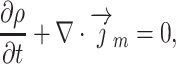
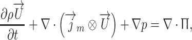
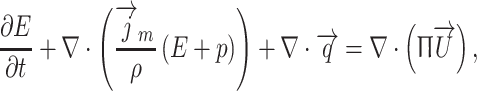
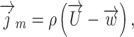
Regularized or quasi-gas dynamic system of equations includes equations of balance of mass, momentum and energy [11, 21]:

1

2

3

4

5

6

where – density; – velocity; - mass flux density; p – pressure; E – total energy per unit volume; - viscous stress tensor; – heat flux; , .- classical Navier-Stokes viscous stress tensor and heat flux; , , - additional dissipative terms [11, 21] in the corresponding equations with coefficient, which is denoted as .

As an extension of the classical system of Navier-Stokes equations, the QGD system contains additional constituents that are proportional to a small coefficient having the time dimension. When parameter tends to zero, QGD system of equations reduces to Navier-Stokes system. In dimensionless form, the value of is proportional to the Knudsen number. For compressible gases, is too small to use its direct value because it does not provide the required stability of the numerical algorithm. In this case, the role of the free path in the numerical algorithm can perform the step of the computational grid:

7

where _QGD is a small constant in the range from 0 to 1, which is the tuning parameter of the numerical QGD algorithm; - computational grid step; a is the sound velocity. When solving problems with high values of Mach and Reynolds numbers, the introduced dissipation with the help of -supplements is insufficient, and therefore additional viscosity is introduced into the system as a coefficient in the viscous stress tensor:

8

where Sc_QGD is a scheme parameter that ensures its stability at high values of local Mach number. Values of _QGD and Sc_QGD are selected as the trade-off between stability of the numerical algorithm and numerical diffusion. The theoretically justified guide on how to select values of coefficients is presented in [22, 23]. The general rule for the adjustment of these coefficients consists in gradual decrease from the baseline configuration: _QGD = 0.4–0.5 and Sc_QGD = 1. According to the definition (7), (8) the decrease of _QGD could be considered as the mesh refinement. According to the previous research [15] the recommended value of _QGD and Sc_QGD are 0.15 and 0, respectively.

The system of Eqs. (1)–(3) is implemented in QGDFoam solver based on OpenFOAM package [24, 25]. More details about the code, including the governing equations can be found in papers [21, 24].

Acoustic Analogy

One of the main approaches used to model acoustic wave propagation is the solution of the Ffowcs Williams and Hawkings equation. There are various integral formulations for solving this equation. In this paper we used the Farassat 1A formulation [26, 27], implemented in the libAcoustics library developed by the authors [28, 29]. More details about the governing equations of this formulation can be found in paper [27]. This analogy is used to determine the far field noise generated by an acoustic source moving in a gas. This formulation is widely used to calculate the acoustic pressure from the rotor or jet flows. The following formula was used to calculate the sound pressure level (SPL):

9

where p_rms is the root mean square sound pressure, p_ref is reference sound pressure.

The developed library based on OpenFOAM package is publicly available and can be compiled independent of any modules of the main package and the type of solvers.

Numerical Setup

The problem of trans- and supersonic jets outflow with the following initial data is considered: M = 0.9, Re = 3600; M = 2.1, Re = 70000. The flow parameters and geometry match an experimental study conducted by Stromberg et al. [18] and Troutt et al. [20] and results will be compared to their data whenever possible.

The computational domain was a rectangular parallelepiped in which the outlet boundary is removed by 100D, the side boundary by 20D, where D is the diameter of the nozzle exit. The inlet boundary corresponded to the exit of the round nozzle and coincides with the beginning of coordinates (see Fig. 1). In addition, the computational grid has been refined on 30D downstream. Based on the recommendations presented in [17], a calculation grid with 40 CPD and a total number of cells of 33 million is constructed. Figure 2 shows a fragment of the grid near the nozzle exit.

Fig. 1.

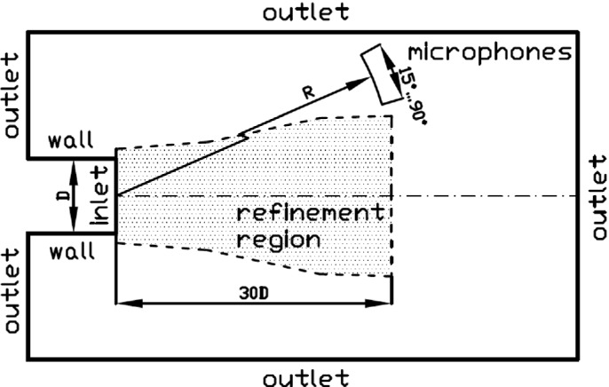
Computational domain and boundary conditions.

Fig. 2.

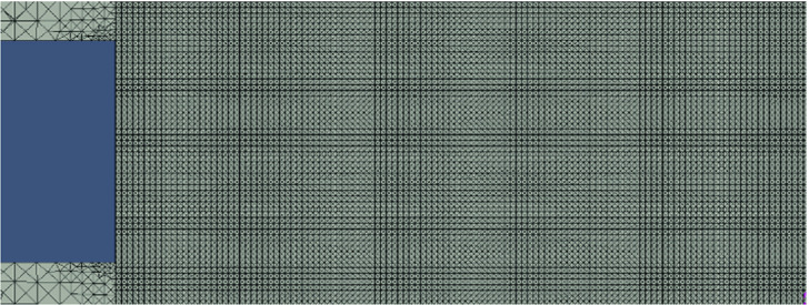
Fragment of the computational grid near the nozzle exit.

The numerical simulation was performed using QGDFoam solver with the following setting parameters defined in [17]: _QGD = 0.15, Sc_QGD = 0. Adams-Bashforth (backward) scheme was used for time derivatives approximation. The turbulence model has not been applied for jet at small Reynolds number. For the case M = 2.1 and Re = 70000, the LES approach with Smagorinsky sub-grid model was used.

The libAcoustics library with Farassat 1A formulation was used to predict acoustic pressure in the far field. Virtual microphones were located at a distance of R = 30D and 40D for jets with low and moderate Reynolds number respectively, the angle of microphones position was set from 15 to 90° to the jet axis.

Results and Discussion

Near Field Calculation

Figure 3 presents the axial distribution of the Mach number averaged over time in comparison with experimental data. Figures 4 and 5 show the flow field of the jets under study.

Fig. 3.

Axial distribution of the mean Mach number: (a) M = 0.9, Re = 3600; (b) M = 2.1, Re = 70000.

Fig. 4.

The jet velocity distribution at M = 0.9, Re = 3600: (a) instantaneous; (b) mean.

Fig. 5.

The jet velocity distribution at M = 2.1, Re = 70000: (a) instantaneous; (b) mean.

The flow field at low Reynolds number is laminar for considerable part of the potential core region. The potential core length of the jet at moderate Reynolds number is between 8 and 10 diameters and characterized by weak shock cell structure. The sonic point in this jet is reached between 18 and 20 diameters downstream of the nozzle exit.

Far Field Noise Prediction

Based on the recommendations [13, 14] on the choice of the form of the control surface to calculate the acoustic pressure from jet flows, two open surfaces were constructed, which are schematically depicted in Fig. 6 (s1 is green, s2 is red). The control surfaces start 0.1D downstream of the inflow boundary and extend to 35D along the streamwise direction. Sound pressure level for two tasks are calculated in terms of a reference pressure scaled to the ambient pressure: 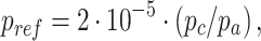where p_c is the pressure in the test chamber, p_a is standard atmospheric pressure.

Fig. 6.

Schematic showing the two open control surfaces surrounding the jet at moderate Reynolds number (Divergence of velocity contours are shown). (Color figure online)

The OASPL directivity distribution for low and moderate Reynolds numbers jets are presented in Fig. 7.

Fig. 7.

Sound pressure level directivity distributions for QGDFoam solver with different control surfaces: (a) M = 0.9, Re = 3600; (b) M = 2.1, Re = 70000.

The results showed that acoustic properties of moderate Reynolds number jet are closely comparable to published in paper [19] of high Reynolds number jet results. The highest levels of generated noise occur at angles around 30°.

The effect of Reynolds number on the acoustic frequency spectrum at the point corresponding maximum acoustic noise are presented on Fig. 8. At the low Reynolds number acoustic spectrum is dominated by a narrow band of frequencies. At the moderate Reynolds number, it is quite full. The broad peak is around that coincides approximately with the low Reynolds condition.

Fig. 8.

Acoustic spectrum in the maximum noise direction ( = 30°): (a) M = 0.9, Re = 3600; (b) M = 2.1, Re = 70000.

Conclusion

The numerical experiments have allowed to investigate the applicability of the developed approach based on implementation of the QGD equations using OpenFOAM package. The developed solver QGDFoam has been coupled with libAcoustics library. Validation of QGDFoam solver was performed on the problems of trans- and supersonic jets of perfect viscous gas and acoustic noise generated by them at low and moderate Reynolds numbers. The calculated gas-dynamic parameters of near-field and acoustic pressure in the far field correspond well with the experimental data.

The analysis of the received data has allowed to expand applicability of QGD algorithms for numerical simulation of the free jet flow at moderate Reynolds numbers. Thus, the resolution of the calculated grid should be at least 40 CPD, and the regularization parameters are Sc_QGD = 0, _QGD = 0.15.

It was found that the jet at moderate Reynolds number both the flow and acoustic properties are considerably more complex than the at low Reynolds number conditions. The major of acoustic noise propagation direction of the investigated jets occur at angles around 30° to the jet axis. The noise spectrum of jet at the low Reynolds number is a narrow band of frequencies in turn at moderate Reynolds number it is quite full.

References

- 1.Crighton DG. Orderly structure as a source of jet exhaust noise: survey lecture. In: Fiedler H, editor. Structure and Mechanisms of Turbulence II. Heidelberg: Springer; 1978. [Google Scholar]
- 2.Tam, C.K.W.: Theoretical aspects of supersonic jets noise. In: NASA, Langley Research Center, First Annual High-Speed Research Workshop, Part 2, pp. 647–662 (1992)
- 3.Baars, W.J., Tinney, C.E., Murray, N.E., Jansen, B.J., Panickar, P.: The effect of heat on turbulent mixing noise in supersonic jets. AIAA Paper, 2011-1029 (2011)
- 4.Tam CKW, Viswanathan K, Ahuja KK, Panda J. The sources of jet noise: experimental evidence. J. Fluid Mech. 2008;615:253–292. doi: 10.1017/S0022112008003704. [DOI] [Google Scholar]
- 5.Tam CKW, Shen H, Raman G. Screech tones of supersonic jets from bevelled rectangular nozzles. AIAA J. 1997;35(7):1119–1125. doi: 10.2514/2.232. [DOI] [Google Scholar]
- 6.Tam CKW, Burton DE. Sound generated by instability waves of supersonic flows. Part 2. Axisymmetric jets. J. Fluid Mech. 1984;138:273–295. doi: 10.1017/S0022112084000124. [DOI] [Google Scholar]
- 7.Tam CKW. Mach wave radiation from high-speed jets. AIAA J. 1984;47(10):2440–2448. doi: 10.2514/1.42644. [DOI] [Google Scholar]
- 8.Kandula M. On the scaling laws and similarity spectra for jet noise in subsonic and supersonic flow. Int. J. Acoust. Vibr. 2008;13(1):3–16. [Google Scholar]
- 9.Tam, C.K.W., Golebiowski, M., Seiner, J.M.: On the two components of turbulent mixing noise from supersonic jets. AIAA Paper, 96-1716 (1996)
- 10.Kraposhin MV, Banholzer M, Pfitzner M, Marchevsky IK. A hybrid pressure-based solver for nonideal single-phase fluid flows at all speeds. Int. J. Numer. Methods Fluids. 2018;88(2):79–99. doi: 10.1002/fld.4512. [DOI] [Google Scholar]
- 11.Elizarova TG. Quasi-Gas Dynamic Equations. Berlin: Springer; 2009. [Google Scholar]
- 12.Chetverushkin BN. Kinetic schemes and quasi-gas-dynamic system of equations. Russ. J. Numer. Anal. Math. Model. 2005;20(4):337–351. doi: 10.1515/156939805775122253. [DOI] [Google Scholar]
- 13.Uzun, A., Lyrintzis, A.S., Blaisdell, G.A.: Coupling of integral acoustics methods with LES for jet noise prediction. AIAA Paper, 4982-5001 (2004)
- 14.Shur M, Spalart P, Strelets M. Noise prediction for increasingly complex jets. Part I: methods and tests. Int. J. Aeroacoustics. 2005;4:213–246. doi: 10.1260/1475472054771376. [DOI] [Google Scholar]
- 15.Kraposhin MV, Epikhin AS, Elizarova TG, Vatutin KA. Simulation of transonic low-Reynolds jets using quasi-gas dynamics equations. J. Phys: Conf. Ser. 2019;1382(1):012019. [Google Scholar]
- 16.Al-Zoubi, A., Beilke, J., Korchagova, V.N., Strizhak, S.V., Kraposhin, M.V.: Comparison of the performance of open-source and commercial CFD packages for simulating supersonic compressible jet flows. In: Proceedings - 2018 Ivannikov Memorial Workshop (IVMEM 2018), pp. 61–65 (2019)
- 17.Epikhin, A., Kraposhin, M., Vatutin, K.: The numerical simulation of compressible jet at low Reynolds number using OpenFOAM. In: E3S Web of Conferences, vol. 128 (2019)
- 18.Stromberg JL, McLaughlin DK, Troutt TR. Flow field and acoustic properties of a Mach number 0.9 jet at a low Reynolds number. J. Sound Vibr. 1980;72(2):159–176. doi: 10.1016/0022-460X(80)90650-1. [DOI] [Google Scholar]
- 19.McLaughlin, K., Seiner, J.M., Liu, C.H.: On noise generated by large scale instabilities in supersonic jets. AIAA Paper, 80-0964 (1980)
- 20.Trouttt TR, McLaughlin DK. Experiments on the flow and acoustic properties of a moderate-Reynolds-number supersonic jet. J. Fluid Mech. 1982;116:123–156. doi: 10.1017/S0022112082000408. [DOI] [Google Scholar]
- 21.Kraposhin, M.V., Ryazanov, D.A., Smirnova, E.V., Elizarova, T.G., Istomina, M.A.: Development of OpenFOAM solver for compressible viscous flows simulation using quasi-gas dynamic equations. In: Proceedings - 2017 Ivannikov ISPRAS Open Conference (ISPRAS 2017), pp. 117–123 (2018)
- 22.Zlotnik AA, Lomonosov TA. Conditions for L2-dissipativity of linearized explicit difference schemes with regularization for 1D barotropic gas dynamics equations. Comput. Math. Math. Phys. 2019;59:452–464. doi: 10.1134/S0965542519030151. [DOI] [Google Scholar]
- 23.Zlotnik AA, Lomonosov TA. L2-dissipativity of the linearized explicit finite-difference scheme with a kinetic regularization for 2D and 3D gas dynamics system of equations. Appl. Math. Lett. 2020;103:106198. doi: 10.1016/j.aml.2019.106198. [DOI] [Google Scholar]
- 24.Kraposhin MV, Smirnova EV, Elizarova TG, Istomina MA. Development of a new OpenFOAM solver using regularized gas dynamic equations. Comput. Fluids. 2018;166:163–175. doi: 10.1016/j.compfluid.2018.02.010. [DOI] [Google Scholar]
- 25.QGDFoam solver. https://github.com/unicfdlab/QGDsolver
- 26.Brentner KS, Farassat F. An analytical comparison of the acoustic analogy and Kirchhoff formulations for moving surfaces. AIAA J. 1998;36:1379–1386. doi: 10.2514/2.558. [DOI] [Google Scholar]
- 27.Brès, G.A., Pérot, F., Freed, D.: A Ffowcs Williams–Hawkings solver for lattice Boltzmann based computational aeroacoustics. AIAA Paper, 2010-3711 (2010)
- 28.Epikhin A, Evdokimov I, Kraposhin M, Kalugin M, Strijhak S. Development of a dynamic library for computational aeroacoustics applications using the OpenFOAM open source package. Procedia Comput. Sci. 2015;66:150–157. doi: 10.1016/j.procs.2015.11.018. [DOI] [Google Scholar]
- 29.libAcoustics library. https://github.com/unicfdlab/libAcoustics