Highlights
-
•
We presented the first review of application of BN in SC risk and resilience.
-
•
We analyzed reviewed journal papers using network analysis and clustering analysis.
-
•
The gaps and future research gaps are identified and discussed.
Abbreviations: BN, Bayesian Network; BP, Backward Propagation; CPT, Conditional Probability Table; DAG, Directed Acyclic Graph; DBN, Dynamic Bayesian Network; EU, Expected Utility; TEU, Total Expected Utility; FMEA, Failure Mode Effects & Analysis; FP, Forward Propagation; MCS, Monte Carlo Simulation; MF, Manufacturing Facility; OEM, Original Equipment Manufacturer; SC, Supply Chain; SCRM, Supply Chain Risk Management; JPD, Joint Probability Distribution
Keywords: Supply chain management, Supply chain resilience, Bayesian network, Machine learning, Ripple effect
Abstract
In the broad sense, the Bayesian networks (BN) are probabilistic graphical models that possess unique methodical features to model dependencies in complex networks, such as forward and backward propagation (inference) of disruptions. BNs have transitioned from an emerging topic to a growing research area in supply chain (SC) resilience and risk analysis. As a result, there is an acute need to review existing literature to ascertain recent developments and uncover future areas of research. Despite the increasing number of publications on BNs in the domain of SC uncertainty, an extensive review on their application to SC risk and resilience is lacking. To address this gap, we analyzed research articles published in peer-reviewed academic journals from 2007 to 2019 using network analysis, visualization-based scientometric analysis, and clustering analysis. Through this study, we contribute to literature by discussing the challenges of current research, and, more importantly, identifying and proposing future research directions. The results of our survey show that further debate on the theory and application of BNs to SC resilience and risk management is a significant area of interest for both academics and practitioners. The applications of BNs, and their conjunction with machine learning algorithms to solve big data SC problems relating to uncertainty and risk, are also discussed.
1. Introduction
Bayesian networks (BN) are probabilistic graphical models, which have been well recognized as a rigorous methodology for the quantification of risks, uncertainty modeling, and decision-making in the presence of structural dynamics (Fenton and Neil, 2013, Qazi and Akhtar, 2018). BNs are rooted in statistics, computer science, and artificial intelligence and were initially introduced by Pearl (1988). BNs are structured using conditional probability and Bayes’ theorem, which capture dependency among system components.
Dependencies in the context of supply chain (SC) management can be modeled in different forms, for example, as a flow of commodities between manufacturer and distribution centers. The material flows can be vulnerable to disruptions and numerous risks (Craighead et al., 2007, He, Alavifard, Ivanov, & Jahani, 2018, Ivanov et al., 2017, Macdonald et al., 2018, Pournader et al., 2020, Yoon et al., 2018) which yield different types of supply, production, and logistics disruptions (Sawik, 2020, Zhong and Nof, 2020). Within SC risk management (SCRM), the resilience paradigm plays an important role. SC resilience has recently gained extensive attention in research. Resilience is commonly understood as the SC’s ability to withstand disruptions and recover after disruption (Blackhurst et al., 2011, Brandon-Jones et al., 2014, Dubey et al., 2019, Hosseini et al., 2019a, Pettit et al., 2019). A resilient SC is therefore characterized by some redundancy (e.g., backup suppliers and risk mitigation inventory) and recovery capabilities (Behzadi, O’Sullivan, & Olsen, 2020; Dolgui, Ivanov, & Sokolov, 2020). One of the dominant challenges in managing SC resilience is controlling the so-called ripple effect, that is, the propagation of a disruption throughout multiple echelons in the SC (Dolgui et al., 2018, Mishra et al., 2019, Scheibe and Blackhurst, 2018). For example, numerous ripple effects have been observed at the beginning of COVID-19 pandemic when disruptions at suppliers in Asia have propagated downstream in the SCs causing material shortages and even facility closures on other continents (Ivanov, 2020a, Ivanov, 2020b). Recent studies have developed and tested different approaches to designing and controlling SC resilience using the BN with consideration of the propagation of disruption (Hosseini & Ivanov, 2019). However, these developments are rather fragmented and existing knowledge is scattered throughout literature.
BNs have been widely used in numerous domains of research, including the energy, defense, and robotics industries (Boutselis and McNaught, 2019, Buritica and Tesfamariam, 2015, Daemi et al., 2012, Lazkano et al., 2007, Munya et al., 2015), social sciences, including ecology (Bac Dang et al., 2019, Lau et al., 2017), medicine (Corani et al., 2013, Flores et al., 2011, Haddawy et al., 2018, Labatut et al., 2004, Petousis et al., 2016, Wang et al., 2019), services and baking (Baesens et al., 2004, De Sa et al., 2018, Gupta and Kim, 2008, Tavana et al., 2018), finance and economics (Gemela, 2001, Kita et al., 2012), etc. Although BNs and the theory underpinning them have flourished in the field of engineering, applications to SCRM and resilience have progressed rather slowly. One of the major reasons for this is the difficulty of generating BNs. For many years, researchers had to build their own BN models. Needless to say, this made BNs unapproachable to the majority of researchers, particularly SCM scholars. During the last decade, several BN software packages were introduced to the market. This has facilitated the implementation of BNs and resulted in increasing interest in research on BN applications to SCRM, risk and resilience (Garvey et al., 2015, Hosseini et al., 2019, Hosseini et al., 2019b, Hosseini et al., 2019a, Ojha et al., 2018).
BNs have unique features that do not exist in other methodologies such as regression modelling (Chaudhuri et al., 2018, Kumar Sharma and Bhat, 2014) failure mode effect analysis (FMEA) (Li & Zeng, 2016), fault tree diagrams (FTD) (Athikulrat, Rungreanganun, & Talabgaew, 2015), Markov chains (Teasley, Bemley, Davis, Erera, & Chang, 2016), Monte Carlo simulations (MCS) (Deleris & Erhun, 2005), and structural equations modelling (Liu, 2012, Sreedevi and Saranga, 2017). This makes them interesting in terms of application to risk analysis and managing uncertainty in complex SCs.
Despite the increasing number of publications on BNs, an extensive review of their applications to SC risk, resilience, and the ripple effect is lacking. To address this gap, we analyzed research articles published in peer-reviewed academic journals from 2007 to 2019 using network analysis, visualization-based scientometric analysis, and clustering analysis. We contribute to literature by discussing the challenges of current research, and, more importantly, identifying and proposing future research directions.
To this end, we organize our study around the following main research questions (RQ), i.e.:
RQ1: What are the merits and challenges of implementing BNs in the context of SC risk, resilience, and the ripple effect?
RQ2: How and when should BNs be used in the context of SC risk and resilience?
RQ3: What are potential subjects of research in SC risk and resilience that can be uncovered through utilization of BNs?
RQ4: How can the ripple effect in SCs be controlled by using BNs?
RQ5: How can BNs be integrated with machine learning to solve big data SC problems?
More specifically, in this study, we argue that BNs are appropriate tools for modelling and measuring SC risk and resilience, as well as controlling the ripple effect. This is especially the case in large, interconnected and complex networks, because BNs 1) capture the interdependency between SC entities, 2) reason with partial or uncertain information, 3) combine expert knowledge with historical data when the source of risk to the SC is novel (e.g., natural disaster) and data availability is limited, 4) incorporate the new information, 5) measure the disruption of upstream entities on downstream entities of SCs, and 6) enable data-driven integration with machine learning techniques. This is the first survey paper that analyzes the applicability and appropriateness of BNs for modelling, measuring, and assessing SC risk and resilience problems.
We demonstrate the merits and limitations of applying BNs to this field of research. In addition, we compare several popular SC risk management approaches to BNs. Last, we discuss potential research opportunities that can be addressed by BNs. The rest of this paper is organized as follows. In Section 2 we present research methodology and data visualization. Section 3 articulates major anchors of the BN theory. In 4, 5, we discuss the studies on BN applications to SC risk and resilience identified through our search. Subsequently, in Section 6 we tease out and generalize research and managerial implications of BN applications to SC risk and resilience. One specific aspect of BN applications, i.e., data learning is discussed in Section 7. We conclude with Section 8 by summarizing major findings and outlining some future research directions.
2. Research methodology and data visualization
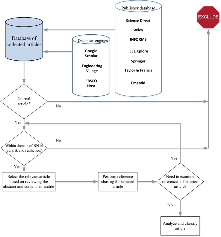
We developed an original framework to analyze literature on the application of BNs to SC risk, resilience, and the ripple effect (Fig. 1 ).
Fig. 1.
Research methodology process framework.
Initially, we selected seven dominant online databases (i.e., Science Direct, Wiley Online Library, Informs, IEEE Digital Library, Springer, Taylor & Francis, and Emerald Publishing). To ensure the depth and breadth of our search, we also used well-known academic databases, including Google Scholar, Engineering Village, and Ebsco Host. We confined the review to existing literature exclusively found in journal articles. Using keywords to perform the search, we selected articles pertinent to the application of BNs in SC risk and resilience. The search process was performed based on a combination of keywords relating to topic and methodology. The main keywords we used for topics included “supply chain risk”, “supply risk”, “supplier risk”, “supply chain resilience”, “resilient supply chain”, “supply chain vulnerability’, “supply chain disruption”, “supply chain risk management”, “supply chain disruption”, “supply chain recovery”, “supply chain risk management”, “supplier risk”, and “supply chain risk uncertainty”. The main keywords we used for methodology included “Bayesian network”, “Bayesian belief network”, “Probabilistic graphical models”, “Bayesian networks”, “BN”, “Bayesian analytical”, and “Bayesian inference”. 63 papers have been found with a publication year between 2007 and 2019. The abstracts and contents of each article were assessed by two independent researchers to ensure that the contents of each were relevant to the scope of this study. For these relevant articles, we performed further reference chasing. We then read the abstracts and contents of references identified in the previous step to ascertain whether they might also be relevant to this study. Further, each article was classified according to the year of publication and the type of journal.
In the further course of this paper, we present a visualization-based scientometric analysis to evaluate the current state and recent developments in BN applications to SC risk and resilience. Data visualization as a tool of the literature review has become increasingly utilized, i.e., Fahimnia et al., 2015, Xiang et al., 2017, Hosseini et al., 2019a, Zhong et al., 2019, Yu et al., 2019. Such an analysis can help to (1) summarize the general characteristics of publication outputs and main subject categories, (2) reveal emerging trends and developments, and (3) identify the share of journals with focused topics.
2.1. Term mapping visualization
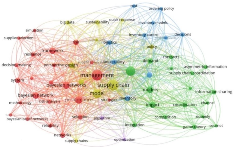
An important objective of visualization is to analyze the frequency of keywords that have been used in literature on BN applications to SC risk and resilience. The term map clustering illustrated in Fig. 2 allows representing the state-of-the-art research angles around which we organize our overview of different subfields and their interconnections in order to identify potential opportunities for fulfilling the research gaps between the subfields.
Fig. 2.
Term map clustering.
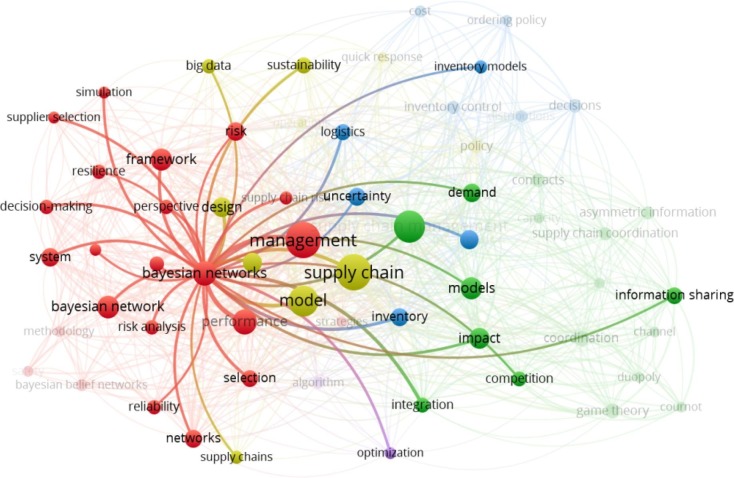
This visualization depicts which terms are most important in a publication cluster and what the relationship of co-occurrence is between these terms (Van Eck & Waltman, 2014). There are five clusters (red, blue, green, yellow, and purple) in the term mapping visualization. Each cluster contains the terms that have the highest proportion of co-occurrence. The distance between two terms is an indication of the relatedness of the terms. The smaller the distance between two terms, the stronger the relatedness is. The relatedness of terms is determined based on co-occurrence in documents. The respective co-occurrences analysis between BN and other terms is represented in Fig. 3 . The co-occurrence mapping represents the link between two keywords (nodes), which is approximately inversely proportional to the similarity (relatedness in terms of co-occurrence) of the keywords (Bornmann, Haunschild, & Hug, 2018).
Fig. 3.
Co-occurrence analysis between BN and other terms.
2.2. Journal co-citation analysis
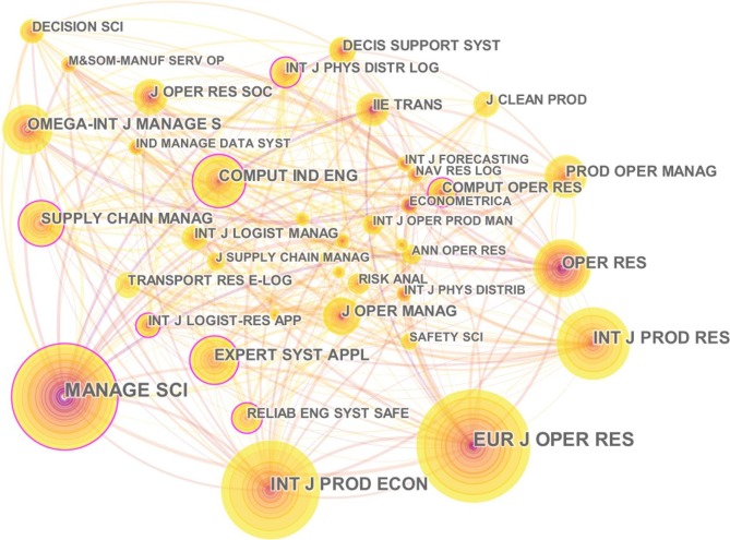
We used CiteSpace to visually cluster in which journals literature on the topic is being published. Journal co-citation analysis helped us to obtain insights regarding the frequency and influence individual journals are having on this field of research (Liu, Yin, Liu, & Dunford, 2015).
According to the journal clustering visualization represented in Fig. 4 , the top 10 cited journals are European Journal of Operational Research, Management Science, International Journal of Production Economics, International Journal of Production Research, Operations Research, Computers & Industrial Engineering, Omega, Expert Systems with Applications, Supply Chain Management, Production and Operations Management, respectively. The visualization indicates that these journals have a greater influence in the field of SC risk and resilience.
Fig. 4.
Visualization of journal co-citation network.
3. Theory of Bayesian network (BN)
This section focuses on understanding the principles of BNs, that is: 1) BN definition, assumption and fundamentals, 2) structural learning, 3) parameter learning, and 4) inference and reasoning.
3.1. Fundamentals
BNs are a powerful technology for capturing uncertainty and assessing risk. BNs are structured based on Bayes’ theorem and conditional probability theory. Bayes’ theorem enables us to reason in a logical, rational, and consistent way by computing the posterior probability of input data given new data input in a specific state. Bayes’ theorem can be represented as shown in Eq. (1):
| (1) |
For data and variable is the posterior probability of in light of the observed data , is the likelihood function of the probability of new data given , is prior (unconditional) probability distribution of parameter , and is marginal likelihood (evidence). With the use of Bayes’ rule and in light of the data, we are able to update our beliefs about the variable to a posterior belief. BNs can be used for representing the impact of evidence on existing data through probabilistic expressions describing the causal relationship among variables (Dury, Valverde-Rebaza, Moura, & Andrade Lopes, 2017).
Technically, BNs are directed acyclic graphs (DAGs) with a set of nodes (variables) and set of arcs (edges), where the probabilistic relationship among variables is expressed by a set of arcs. Variables in BNs can be defined in different forms, including Boolean (yes/no, true/false), continuous, ranked (low/medium/high), etc. Let’s consider a BN with a set of nodes, represented by , and set of arcs that specifies the probabilistic dependency among variables. Let’s assume that there is outgoing arc from to , indicating a relationship where the state values of variable depend on state values of variable . In the context of risk management, if we consider and to both be disruptive events, then the occurrence of depends on the occurrence of . Put simply, and are cause and effect variables. is called the parent of because of the outgoing arc from to , while is called the child of . There are three types of nodes in BNs: 1) leaf nodes, which are nodes without a child, 2) root nodes, which refer to nodes without a parent node, and 3) intermediate nodes, are nodes with at least one parent and one child node.
Consider a BN with 4 nodes as illustrated in Fig. 5 .
Fig. 5.
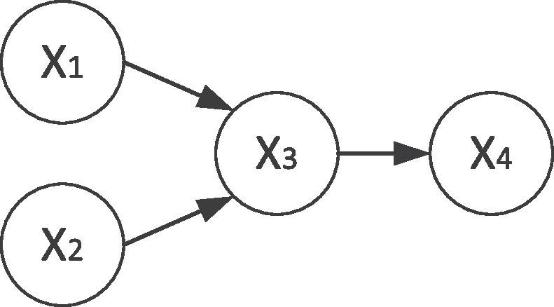
Example BN with 4 nodes.
In the example in Fig. 5, and are root nodes, is intermediate node, and is a leaf node. The prior probabilities of , and the conditional probabilities of , and must be determined. Each node is associated with a conditional probability table (CPT), which lists the probability of a realization of a variable given the values of other variables.
The probability of individual variables can be computed from the joint probability distribution (JPD) in a BN. The JPD of this BN can be written by Eq. (2).
| (2) |
Suppose that we are interested in calculating the probability of , then can be calculated using Eq. (3).
| (3) |
Consider a supplier that may fail to deliver raw materials to a manufacturer due to two disruptive events, e.g., hurricane and labor strike, denoted by , and , respectively, as shown in Fig. 6 . The supplier is a Boolean variable with the states “failed” or “operational”. There are two states (true/false) associated with each disruptive event. The true and false states represent the probabilities that the disruptive event occurs and does not occur, respectively.
Fig. 6.
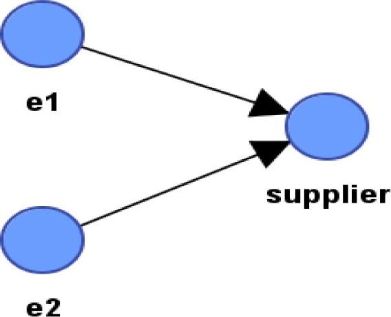
BN for modeling supplier disruption.
Consider prior probabilities of independent occurrence of the hurricane and labor strike as 4% and 7%, respectively. The probability of disruptive events can be obtained through historical data or expert knowledge, or a combination of both thereof. The probability of a supplier failure is conditional on the probability of the occurrence of disruptive events and . The CPT of the supplier given and is shown in Table 1 .
Table 1.
The CPT of supplier disruption given two disruptive events.
| Disruptive event 1, e1 (hurricane) | true |
false |
||
|---|---|---|---|---|
| Disruptive event 2, e2 (labor strike) | true | false | true | false |
| Supplier fails | 0.21 | 0.08 | 0.12 | 0.02 |
| Supplier operates | 0.79 | 0.92 | 0.88 | 0.98 |
The disruption probability of supplier is calculated based on the JPD using Eq. (4).
| (4) |
In the example given, the probability that the supplier fails or operates is 2.95% and 97.05%, respectively, as shown in Fig. 7 .
Fig. 7.
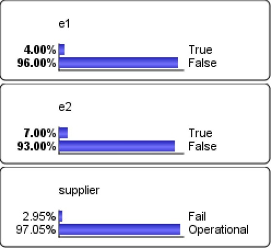
Distribution probability of variables associated with BN model in Fig. 6.
3.2. Structural learning
Perhaps the most difficult task in dealing with BNs is understanding how they are structured. Generally speaking, the BN structure (configuration) can be determined using expert knowledge or through machine learning algorithms (Koller & Friedman, 2012). The intuitive knowledge provided by experts can determine dependencies between the variables, that is, the event likelihoods (i.e., variable assignments). In this case, the BNs can be constructed manually. In other cases, the use of expert knowledge in BNs with large numbers of variables (nodes) may not be easy or practical. In some cases, it can be difficult to identify experts with all the required knowledge.
An alternative way to determine the structure of a BN is through data. This means that the causal relationships (dependency) among variables are determined through data learning. Generally, there are two methods of structure learning. The first is a score-based approach, which uses a scoring function such as “maximum likelihood” to assess how well the BN fits to the data, and then searches over the space of DAGs to find the structure with the highest score. The score-based approach is comprised of two parts: the search algorithm and the definition of a score metric. Local search, greedy search, and the Chow-Liu algorithm are among the most common search algorithms that have been applied in this approach (Conrady & Jouffe, 2018). The second method is a constraint-based approach, which employs statistical tests to identify a set of link constraints for the graph and then finds the best DAG that satisfies the constraints. Notably, searching for the optimal BN structure is NP-hard problem. Hence, there have been several attempts to reduce the search space for different structure learning techniques (Friedman, Nachman, & Peer, 1999).
3.3. Parameters learning
For a given BN structure and the CPT of node i, is typically estimated using the maximum likelihood expectation method from the observed frequencies in the dataset associated with the BN. When a dataset is not available, CPTs can be determined using expert knowledge.
3.4. Inference and reasoning
The ability of BNs to perform inference is one of their most powerful features. This fact makes BNs suitable for analyzing SC risk and resilience problems. The inference in BNs relies upon evidence. The inference analysis can be performed by entering evidence and using propagation to update the marginal probabilities of all unobserved variables. Consider the BN example with 5 nodes illustrated in Fig. 8 . Let’s assume that nodes to are Boolean with two states of false and true, and is a Boolean node with states of yes and no.
Fig. 8.
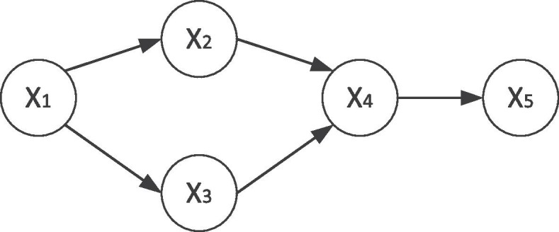
BN example with 5 nodes.
Assuming that we have evidence that node is in its yes state, we wish to know the probability that is true given is yes. This probability can be calculated as shown in Eq. (5).
| (5) |
Different methods exist to reduce the complexity of the marginalization expressions in Eq. (5). These include Monte Carlo sampling, dynamic programming, and loopy belief propagation (see, e.g., Fenton & Neil, 2013 for a detailed discussion).
4. Applications of BNs to supply chain risk management
During the last two decades, SCs have become more vulnerable to disruptions due to globalization, multiple sourcing strategies, complexity, and interconnectedness (Craighead et al., 2007, Ho et al., 2015, Hosseini et al., 2016a). Blackhurst and Wu, 2009, Sodhi and Tang, 2010, Zsidisin and Ritchie, 2010 identified a framework based on four key steps to reduce SC vulnerability to disruptions: (1) identifying potential risks, (2) measuring and assessing risks, (3) mitigating risks, and (4) responding to risks. Measuring potential SC risks is essential to reducing the disruption of SC operations. For example, Hong, Lee, and Zhang (2018) presented a comprehensive review on procurement risk management under uncertainty. Their findings indicate that a proper management of procurement risks is not only required to mitigate lead time and price risks but also emphasizes the value of sophisticated analytical techniques in managing supply and demand uncertainties.
The focus of this section is to review the applications of BN on modelling and measuring SC risks. This section does not aim to review the definitions of risks and analyze SC risk factors. We refer readers to Ho et al., 2015, Fahimnia et al., 2015, Heckmann et al., 2015, Ivanov and Dolgui, 2019 for a comprehensive review of definitions and core characteristics of SC risks.
4.1. SC risk modeling
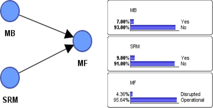
Consider a manufacturing facility (MF) whose operation is exposed to two major disruptions: machinery breakdown (internal risk) and shortage of raw material (external risk). These two disruptions can negatively impact the operations of an MF (Fig. 9 ).
Fig. 9.
BN of manufacturing facility (MF) impacted by two risks and their corresponding distribution probabilities.
The BN illustrated in Fig. 9 has two parent nodes, machinery breakdown and shortage of raw material, denoted by MB and SRM, respectively, and a child node represented by MF. Each parent node consists of two states: yes versus no. Each disruption occurs independently and there is no correlation between disruptions. Let’s assume that the prior probability that MB and SRM risks occur independently are 7% and 9%. An MB and SRM risk induces 10% and 12% probability of disruption at MF, respectively. The probability that MF fails to operate when both risks occur simultaneously is 28% and there is still a 3% chance that MF will fail to operate if neither MB nor SRM occurs. The marginal probability of disruption of MF, is calculated as shown in Table 2 .
Table 2.
Computations of marginal disruption probability of MF.
| State of parent nodes () | ||
|---|---|---|
BN applications to SC risks can be found in numerous studies. Srikanta Routroy (2016) developed a BN to model information risk in SCs. The proposed BN model captures three key risk factors, including information breakdown factors, information leakage factors and reluctance in information sharing factors. The sub-causes of each above-mentioned risk factor are identified and modeled as parents of relevant risk factors. The author then measured the impact of risk factors and their corresponding sub-risk factors in terms of revenue impact. Rodgers and Singham (2019) constructed a BN to evaluate the likelihood and impact of disruptions on a clinical SC network. Their BN model would enable practitioners to develop SC risk mitigations by simulating different possible disruptions in a clinical SC. The BN model used in Rodgers and Singham (2019) is constructed based on expert knowledge elicitation and can be used to identify and prioritize the vulnerable components of SC network.
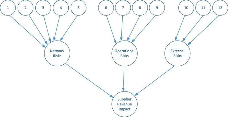
Lockamy and McCormack (2012) used a BN to develop supplier risk profiles to determine the risk exposure of a company’s revenue. The target node in their model is supplier revenue impact, which is conditional on three nodes, network risks, operational risks, and external risks, as represented in Fig. 10 . Each risk itself is conditional on a set of relevant sub-risks. For example, operational risks are conditional on driving risk factors (risks 6–9 in Fig. 10), which include quality problem, delivery problem, service problem, and supplier human resource problem. The authors then investigated the supplier’s revenue impact subject to various combinations of network, operational, and external risks. The authors examined and ranked the vulnerability of 15 suppliers with respect to network, operational, and external risks. The practical implication of their model is to assist SC managers in identifying the most vulnerable suppliers.
Fig. 10.
BN for analyzing the risk profile of supplier revenue impact (Lockamy & McCormack, 2012).
Kaki, Salo, and Talluri (2015) evaluated the risks of an automotive SC using BN methodology. The authors proposed index, called supplier disruption impact (SDI), which measures the increased total risk of a focal manufacturing company (FMC), when supplier n is disrupted. The authors studied the impact of SC complexity, density, and reliability using BNs. Managerial insights reflect how SC complexity and density impact the risks that stem from the supply base. The authors also compared the vulnerability of a single supply strategy versus a multiple supply strategy using BNs. The authors concluded that a supplier with a large number of parents is more risky which indicates that suppliers with more parents have higher importance. The proposed BN model can be only implemented for forward SCs but it cannot be used for the revere SCs as they contain cycles. Besides, the authors built BN model based on an assumption that a supplier can be either fully disrupted or fully operational. This could not be the case in practice as a supplier can be still operational with some level of its original capacity in the presence of a disruption. As such, modeling states of a supplier disruption with ranked variables (i.e., operational, fully operational, semi-operational) could extend the results of this study.
Kumar Sharma and Sharma (2015) developed a BN to quantify the risk of a SC system. The authors considered four major risk factors, including firm specific (process risk, control risk), industry specific (supply risk, demand risk), SC specific (relationship risk, logistical risk), and risk of natural disaster. One major critical point is that the weights of all SC risks are considered equally. It is notable that SC risk factors (i.e., demand risk, environmental risk, and operational risk) may have different importance and therefore the disruption impacts on suppliers can vary. Utilizing a weighted ranked node that captures the weight of each risk could strengthen the usability of the proposed BN model. Besides, utilizing a continuous node instead of a binary variable could be more practical.
The main critical observations from Lockamy and McCormack, 2012, Kumar Sharma and Sharma, 2015, Kaki et al., 2015, Srikanta Routroy, 2016 is that the interdependency among risks is almost ignored. The focus of those works on a particular problem without adapting BNs to the reality of SCRM needs to be extended by capturing the complex interdependency among different types of SC risks. Moreover, the likelihood of an SC risk is the only associated factor considered, while the severity and detection stage (i.e., early/late) of a disruption risk are not taken into account.
Corman and Kecman (2018) developed a BN to predict the delay of a train due to common disruptions which impact railway transportation systems. The proposed BN model enables the probability of distribution due to random variables to be updated and the uncertainty of future train delays to be reduced. The model helps decision makers to make better predictions of train traffic. Wan, Yan, Qu, and Yang (2019) proposed an integrated BN and FMEA to assess maritime SC risks. The main advantage of their method is to improve the accuracy of estimating maritime SC risk in the presence of data with high uncertainty. The authors considered five common maritime SC risks including transportation of dangerous goods, fluctuation of fuel price, fierce competition, unattractive markets, and change of exchange rates in sequence. Every risk factor is conditioned on five triggers including likelihood, time delay, additional cost, quality damage, and visibility. Rodger (2014) applied a BN for estimating SC backorder aging risk. The authors determined the structure of BN model from real-world SC data and the posterior distribution probability for backorders are determined using a stochastic simulation based on Markov blankets. The BN is used to minimize the replenishment cost by finding optimal backorder replenishment alternatives.
Qazi, Dickson, Quigley, and Gaudenzi (2018) developed an approach based on integration of a BN and expected utility (EU) to manage SC risks. The main advantage of their BN model is that it considers the risk-aversion of decision makers. The risk acceptance level for risk-averse SC managers, risk-seeking SC managers, and risk-neutral SC managers is modeled using a BN. The authors considered j risks imposed on the SC network. The risk propagation measure (RPM) for the jth risk is defined as the probability weighted by expected utility of the SC network if risk j is realized. is calculated as shown in Eq. (6).
| (6) |
where is the expected utility given risk j is realized. The authors considered K strategies to mitigate disruption risks. Let denote the kth mitigation strategy, while the mitigation strategy has I states. It is assumed that there is a cost associated with each mitigation strategy, so the EU resulting from undertaking risk mitigation strategy k can be calculated using Eq. (7).
| (7) |
where is the probability that strategy type k is in state i, and is the utility associated with mitigation strategy k, and the cost of mitigation strategy k. The authors finally studied the impact of different risk mitigation, risk sources, and risk interaction using BN. The proposed BN in Qazi et al. (2018) modeled only on-time state of the supply risk rather than monitoring the dynamic nature of the SC risk. In addition, this BN model does not capture the conflicting motivation of main stakeholders. Other BN applications to SC risk assessment can be found in Kao et al., 2005, Wu, 2005, Li and Chandra, 2007, Shevtshenko and Wang, 2009, Sharma and Routroy, 2016, Kumar Sharma and Sharma, 2015.
4.2. Interdependency modeling of SC risks
A major research gap in the field of SC risk management is the interdependency impact of different risks on SC performance. BNs are powerful tools for capturing the interdependencies among risks and their impacts on SC performance. The earthquake and tsunami that struck the northeast coast of Japan in 2011 halted the operations of many automotive and electronic manufactures and suppliers for several weeks (Computerworld., 2016, Reuters., 2016). The Japanese tsunami was triggered by the earthquake. The impact of this interdependency was ignored, so the occurrence of the tsunami and its impact was not predicted at an early stage (Livescience, 2013, Nature, 2011).
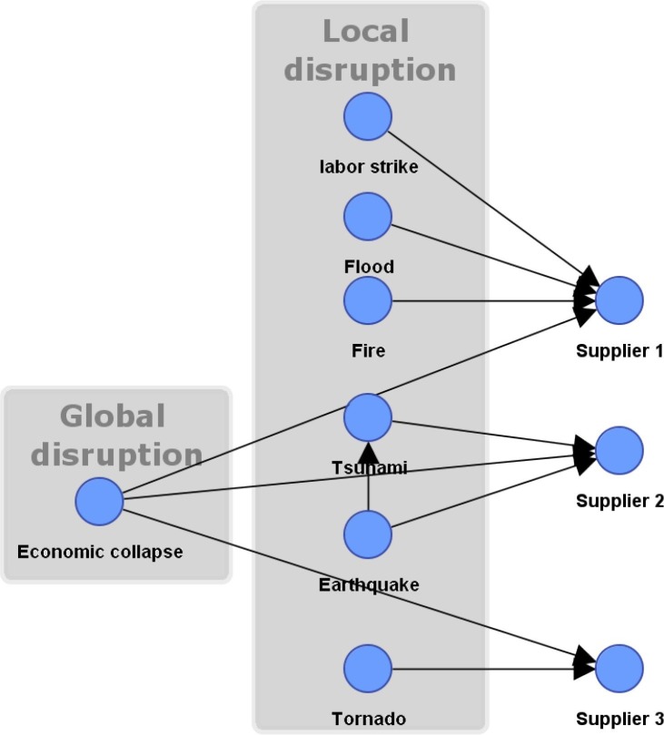
Through conditional probability, risk interdependency can be easily modeled using a BN. We demonstrate a BN model in Fig. 11 with three suppliers that are impacted by global disruption, local disruption, or combination of both thereof.
Fig. 11.
Local and global disruptions with consideration of risk interdependency.
Supplier 1 is impacted by three local disruptions. Supplier 2 is impacted by two local disruptions: tsunami and earthquake. The tsunami is conditional on the earthquake, so the tsunami can directly disrupt supplier 2, and or the occurrence of an earthquake could indirectly disrupt supplier 2 through tsunami. Supplier 3 is impacted by a single local disruption. Finally, all suppliers are vulnerable to a global disruption, economic collapse. As demonstrated in this example, a BN is not only capable of modelling the different types of SC risks (local and global), but also the interdependency among those risks.
4.3. SC risk propagation and ripple effect modelling
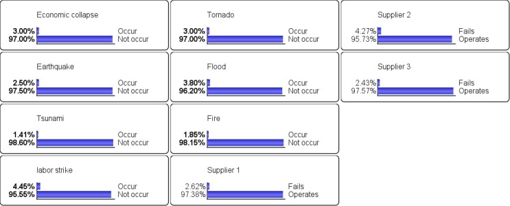
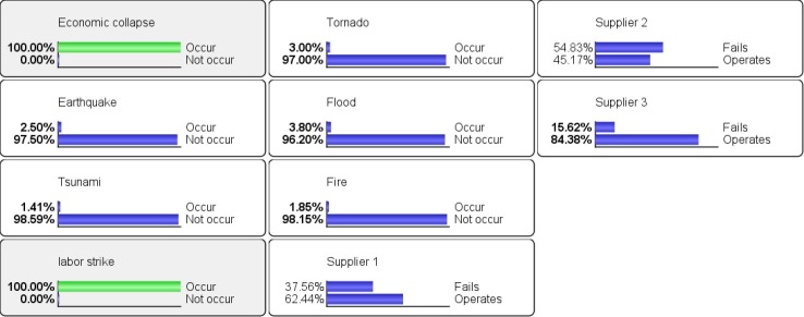
Inference analysis is a unique feature of BNs that can be used to simulate the propagation impact of a disruptive event on SC entities, i.e., the ripple effect (Ivanov et al., 2014, Dolgui et al., 2018, Hosseini et al., 2019b, Mishra et al., 2019). In inference analysis, we enter any number of observations anywhere in the BN model and use propagation to update the marginal probability distribution of all unobserved variables. The inference analysis is usually in the form of forward propagation (FP) or backward propagation (BP). FP and BP are also known as forward and inverse inference, respectively. FP focuses on inferring outputs from input observation, also known as cause to effect propagation, while diagnosis refers to inferring inputs from outputs, also known as effect to cause propagation. We demonstrate FP analysis when economic collapse and labor strike occur, as known through certain observation. The probability failure of suppliers 1, 2, and 3 after FP increases from 2.62%, 4.27%, and 2.43% (Fig. 12 ) to 37.56%, 54.83%, and 15.62%, respectively (Fig. 13 ).
Fig. 12.
Probability distribution of BN model illustrated in Fig. 7.
Fig. 13.
Probability distribution of BN model illustrated with inference analysis on economic collapse and labor strike variables.
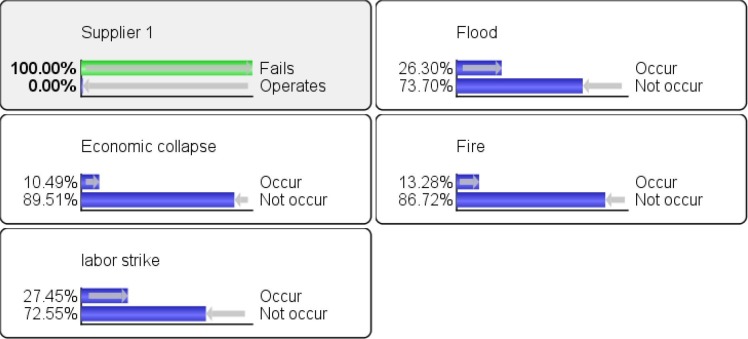
Now we wish to see how much the probability of local and global disruptions increases when supplier 1 (effect) is assumed to be failed. It is notable that any of the three suppliers can be chosen to demonstrate the effect, but we picked supplier 1, because it is impacted by four different disruptive events. BF is performed on supplier 1 by assuming that supplier 1 fails to operate and the impact of this observation is backwardly propagated through the BN by updating the marginal probability distribution of disruption variables. There are different algorithms that can be used for FP and BP analysis, such as variable elimination, relevance tree, loopy belief propagation, and likelihood sampling (Fenton & Neil, 2013). Fig. 14 shows the probability distribution of disruptions that impact supplier 1 under BP analysis.
Fig. 14.
Probability distribution of disruptions impacting supplier 1 under BP analysis.
FB and BP are great features of the BN, because they enable the investigation of the ripple and bullwhip effect on the SCs (Dolgui, Ivanov, & Rozhkov, 2020). The ripple effect occurs when the impact of disruption on upstream entities (suppliers) of a SC cannot be localized, propagate throughout the SC, and negatively impact downstream entities (retailers and customers) (Ivanov et al., 2014, Ivanov et al., 2019a, Ivanov et al., 2019b). A key challenge in the field of SC risk management is to quantify and simulate the impact of disruption on upstream entities and the cascading effect on downstream entities. This can be easily managed using the FP feature of BNs. Recently, several attempts have been made to study the propagation analysis of disruption in SC systems using BNs. Ojha et al. (2018) developed a risk exposure index using the BN approach to model risk propagation in SCs. The authors argue that understanding the cascading impact of risks is critical for designing resilient SC networks. The authors investigated the vulnerability of multi-echelon SC networks against different disruption scenarios that propagates from upstream to downstream nodes.
Nepal and Prakash Yadav (2015) proposed a model based on integration of a BN and a decision tree to evaluate a supplier’s risk. The target node of the BN model is total cost due to sourcing risk, which is conditional on supplier nodes, where each supplier node is conditional on a set of risk factors. The authors used linguistic variables (low, medium, and high) to express the risk level of each risk factor. Many of the BN models (Kumar Sharma and Sharma, 2015, Lockamy and McCormack, 2012, Nepal and Prakash Yadav, 2015, Sharma and Routroy, 2016) that have been proposed in SCRM suffer from ah lack of studying specific risks at particular locations in SCs, the impact of disruption risk throughout the SCs and ultimate consequences. Garvey et al. (2015) proposed an index that measures the risk propagation in a supply networks using BN tool. Their model accounts for the inter-dependencies among different risks, as well as the idiosyncrasies of SC network structure. The authors finally argued that a BN is a natural fit for examining risk propagation in complex and highly interdependent SCs, regardless of the structure of SC networks.
Hosseini et al. (2019b) proposed a metric to measure the ripple effect in a two-echelon SC with a set of suppliers and manufacturers. The authors first defined the operability of each supplier using three states: fully operational, semi-disrupted, and fully disrupted. The service level of a supplier is then defined as the child node of the supplier, meaning that the service level depends on the operability level of supplier. The authors modeled the ripple effect of supplier disruption in terms of the total expected utility (TEU) of a supplier. The TEU of a supplier is modelled using a decision tree, which is created based on service level and operability level of that supplier. Fig. 15 represents the TEU of a supplier impacted by its operability and service level.
Fig. 15.
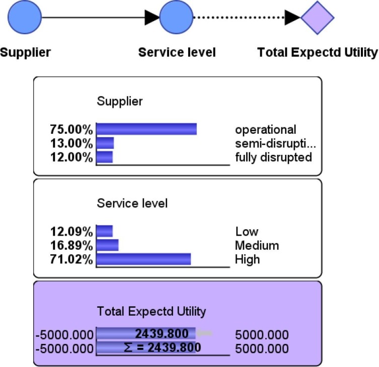
TEU of a supplier created using a BN (Hosseini et al., 2019d).
The TEU of SC is then calculated as the sum of the TEU of all suppliers and the manufacturers. For example, the TEU of set of suppliers is calculated using Eq. (8).
| (8) |
where, is the probability that supplier i is in state k in time period t, denotes the probability that the service level (SL) of supplier i is in state l at time t knowing that supplier i is in state k, and is the expected utility associated with service level state l of supplier i when supplier i is in state k at time period t. There are four set of time periods, suppliers, states of supplier (operational, semi-disrupted, fully disrupted), and states of supplier’s service level (low, medium, high), which are denoted by t, i, k, and l, respectively.
The authors examined the vulnerability of the manufacturer in terms of service level and TEU with respect to disruption of each individual supplier using FP. By performing FP analysis, the authors assumed that each supplier is fully disrupted (fully disrupted = 100%) separately and propagate the impact of this disruption on the service level and TEU of the manufacturer. The FP analysis helped to identify the suppliers whose disruption would have a higher negative impact on service level and TEU of the manufacturer. In Hosseini et al. (2019b), an integrated model of discrete Markov chain and BN is presented in which the impacts of a disruption are quantified in terms of service level and expected utility. The proposed integration of BN with continuous Markov chain model when supplier capacity in the presence of a disruption could be a promising future avenue of research. Qazi, Quigley, and Dickson (2014) proposed a hybrid BN game theory approach, where a BN is used to capture the dependency between risk factors of SC and game theory is utilized to evaluate the risks associated with conflicting incentives of stakeholders within a supply network. Future research should focus more on exploration of hybrid BN approaches with other risk analysis methodologies. The authors presented two different BNs; one representing the Boeing’s perceived SC risks and the other depicting real time supply chain risks faced by the company (Qazi et al., 2014). A game between two suppliers and Boeing are modeled by the authors. Game theory approach is used to model the risks associated with conflicting motivations among the stakeholders in supply networks. The results of this game-theoretical analysis were fed as inputs to the BN.
4.4. A generic BN model for assessing SC risk
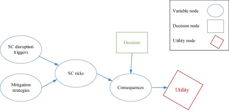
Literature analysis reveals that the existing BN models are developed for specific types of SC structures or specific risks. As such, the literature lacks a generic BN model that can be used regardless of SC structural designs or risk types. The proposed generic BN model is illustrated in Fig. 16 .
Fig. 16.
Generic BN model for assessing SC risk.
In Fig. 16, the distribution probability occurrence of SC risks can be defined using binary states such as true (if the SC risk occurs), and false (if the SC risk does not occur). The SC risk itself can be further broken down into operational and disruption risks or external and internal risks. The SC risks variable is conditional on SC disruption triggers, which include a vast variety of causes, including natural disasters, bankruptcy of supplier or logistics provider, poor communication and information sharing between SC entities, economic and political crises, etc. The occurrence of SC disruptions also depends on the mitigation strategy, which can be viewed as a control variable. SC managers can significantly reduce disruption frequency by utilizing appropriate mitigation strategies, such as high flexibility (flexible transportation modes), redundancy (holding excess inventory backup), and a multiple sourcing strategy (IvanovDolgui, 2019). The probability that a SC risk occurs (True) can be written as shown in Eq. (9).
| (9) |
The consequences of SC risk disruption include increases in lead time, delivery delays, loss of market share, and reputation, etc., which have adverse effect on the utility of SC systems. Hence, utility is considered a child node of the consequences node. The severity of consequences depends on the type of SC risk and managerial decisions. The generic framework represented in Fig. 16 can be tailored for a specific SC, such as a green SC (GSC), depending on the type of SC risk, mitigation strategy, and the consequences of disruption.
The maximal EU of the generic BN model can be calculated as shown in Eq. (10).
| (10) |
5. BN for SC resilience
SC risk management is rooted in an event-oriented perspective while SC resilience is a system property which allows absorbing negative events (risks) and recovering in case of disruptions. One can compare risks with viruses, and resilience - with immune systems. Measuring and analyzing SC resilience has grown significantly as a research topic over the last decade (Cardoso et al., 2015, Hosseini et al., 2019a, Ivanov, 2020, Kim et al., 2015). BNs have been widely used to model and measure the resilience of different systems, such as waterway transportation (Hosseini & Barker, 2016a), urban infrastructure (Huck & Monstadt, 2019), manufacturing (Hosseini et al., 2016a, Rajesh, 2018), and energy (Gupta et al., 2019, Mola et al., 2018). However, the application of BN to SC resilience is relatively new and requires more exploration.
Hosseini and Barker (2016b) developed a BN model to evaluate and select resilient suppliers. The authors measured the resilience of a supplier in terms of its resilience capacity, which consists of absorptive capacity, adaptive capacity, and restorative capacity. The drivers of absorptive capacity include segregation, surplus inventory, backup suppliers, physical protection. The driver of absorptive capacity is rerouting, and the drivers of restorative capacity are technical resources and budget resources. A major critique on this work is that the resilience of a supplier is measured in static time, while a dynamic BN model seems to be more promising.
Ojha et al. (2018) quantified SC resilience through risk propagation analysis. The authors developed a BN model that quantified risk propagation behaviors at each node across the SC network. The resilience of supply network is quantified in terms of loss of service level.
Hosseini and Ivanov (2019) proposed a metric for the resilience of an original equipment manufacturer (OEM) with an assessment of supplier’s vulnerability to disruption and the SC’s exposure to the ripple effect. The resilience of OEM with respect to i-th supplier is measured as the ratio of recoverability to vulnerability of OEM when the i-th supplier is disrupted. The authors quantified the resilience of OEM with respect to each individual supplier on a two-tier automotive SC and measured the importance of each supplier using information theory technique. Finally, they identified a set of suppliers who are important, but less resilient. The outcomes of their research can assist SC managers in enhancing the resilience of their SCs by (i) identifying critical suppliers, and (ii) investing in critical suppliers with low levels of resilience.
Proposed a resilience measure to quantify the resilience of a two stage SC made up of suppliers and single manufacturer using a BN. Resilience () is measured as the union of successful mitigation (pre-disaster) and contingency (post-disaster) strategies, as demonstrated in Eq. (11). Resilience can be achieved when the mitigation strategy harnesses the shocks of disruption, otherwise contingency strategy comes into play.
| (11) |
The probability of successful mitigation is further measured in terms of probability of successful absorptive capacity, while the probability of successful contingency is quantified by the probability of adaptive and restorative capacity (Eq. (12)).
| (12) |
The authors then used BN methodology to model the causality between absorptive, adaptive, restorative capacity and the characteristics of disruptive events (likelihood of disruption, , and intensity of disruption, ) (Fig. 17 ).
Fig. 17.
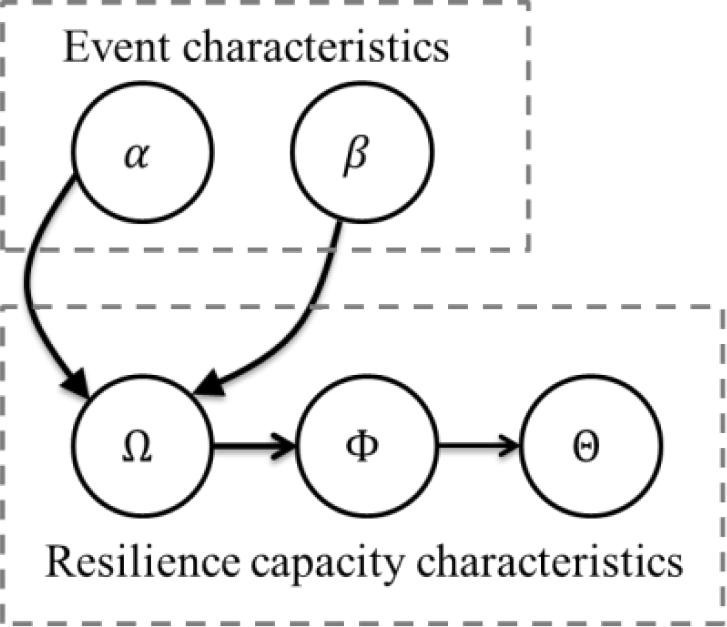
Causal relationship between disruptive event characteristics and resilience capacity characteristics.
As illustrated in Fig. 17, the restorative capacity (third line of defense), denoted by is conditional on adaptive capacity (second line of defense), denoted by , where adaptive capacity itself is conditional on absorptive capacity (first line of defense), denoted by . The likelihood and density of disruption is dependent on absorptive capacity, since it is the first line of defense (pre-disaster strategy).
Ojha et al. (2018) proposed a resilience metric in which the resilience of a supply network with a set of nodes and arcs is calculated in terms of service level. Let’s assume that and represent the service level of node k in week w, and service level of node k when there is no disruption. Finally, denotes the week in which disruption occurs at the supply network, and represents the time when disruption ends plus time to recover from the negative effect of disruption. The resilience index (RI) is then calculated by Eq. (13).
| (13) |
6. Research and managerial implications of BN application to SC risk and resilience
In this section, we summarize research and managerial implications of BN application to SC risk and resilience.
6.1. Research implications
Through our study, we have identified that BNs have several methodical characteristics that make them appropriate for modelling, measuring, and analyzing SC risk and resilience studies. However, BNs also have some potential limitations. This section provides an overview of the strengths and weaknesses of a BN approach to SC risk and resilience modelling and compares it with other methods.
The practical and methodological strengths of BNs can be summarized as follows:
-
1.
Forward and inverse inference: BNs provide a conceptual line of reasoning from cause to effect (forward inference) and effect to cause (inverse inference), and quantify the strengths of those relationships. This unique capability of BNs provides a means to improve decision-making support, since it enables insightful “what-if” disruptive scenarios and provides managers with the ability to investigate potential disruptive evidence. With the assistance of forward inference, decision-makers can predict the impact of SC risks and propagate their impacts on SC performance (e.g., cost, lead time, service level). Inverse inference is particularly beneficial when SC managers wish to know how mitigation strategies (e.g., extra pre-positioning inventory of suppliers, utilizing backup supplier) should be adjusted to efficiently mitigate disruptions.
-
2.
Data type modelling: In contrast to regression, optimization, and neural networks that are only capable of quantitative data, BN models are able to incorporate different types of variables, including Boolean (e.g., true/false), ranked (e.g., low/medium, high), continuous (e.g., normal distribution), and ordinal. BNs are a powerful methodology for capturing the qualitative and quantitative characteristics of SC risks.
-
3.
Small and incomplete dataset: A challenging issue in measuring the resilience of SC systems is the lack of datasets. High impact disruptive events, like natural disasters, occur rarely, and as a result, there are an inadequate amount of datasets in terms of quantifying SC resilience. A useful feature of BNs is that they can easily work with little data. There is no minimum sample size required to perform the analysis, and BNs take into account all data available (Myllymaki et al., 2002, Uusitalo, 2007). Moreover, Kontkanen, Myllymaki, Silander, and Tirri (1997) demonstrate that BNs can achieve good prediction accuracy with rather small sample sizes. Furthermore, BNs have been shown to be robust to imperfect knowledge (Pollino & Handerson, 2010).
-
4.
Combining different sources of knowledge: A key feature of BNs is that they use prior information. Priors reflect our knowledge of the subject before research is conducted, and can be either informative, if there is already sufficient knowledge about the subject, or uninformative, if not much is known (Uusitalo, 2007). Prior probabilities are updated with new data to obtain a synthesis of the old knowledge and new data. This synthesis can be then used as a prior in a new study (Uusitalo, 2007). BNs can easily synthesize historical data and expert knowledge in a mathematically coherent manner. This feature of BNs is useful for SC risk and resilience analysis, because expert knowledge can be combined with a small amount of historical data when there is little data available about disruption characteristics (e.g., probability of disruption, intensity of disruption, consequence of disruption).
-
5.
Complexity: BNs can integrate information from difference sources, model the causality among the elements of SCs, and incorporate both qualitative and quantitative evidence without losing the uncertainties associated with evidence. For example, a BN can be used to capture the interactions between organizational, technical, and human risk factors of SC systems. BNs are suitable tools for exploring and explaining complex SC systems, particularly SC 4.0, the next generation of digital SCs, which are characterized by a high level of interaction (dependency) between humans, cyber-physical systems, and digital technology (Dubey et al., 2019).
-
6.
Explicit handling of uncertainty: It is easy to encode uncertainty and decision freedom into a BN. For example, consider that a model for predicting SC risk disruption is established, but we know that humans do not always make rational decisions. The SC decision-maker could be either risk-averse, risk-seeking, or risk-neutral, might have short/long term objectives in mind when making these decisions, and their decisions might not align with the most rational decision made by the BN model. Here, we can add variables that incorporate the risk aversion of SC managers and a degree of randomness in decisions to obtain a better understanding of how decision-makers in SCs interact with model outcomes. As such, BNs can help to encode the degree of randomness associated with the disruption of SC systems.
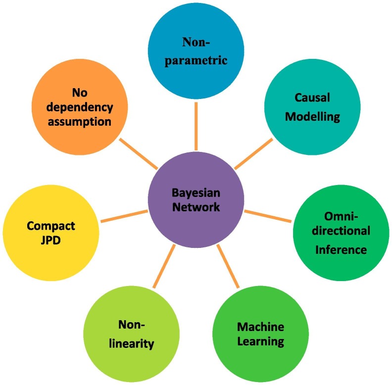
The main features of BNs, which make them attractive for application to SCRM and resilience problems, are summarized in Fig. 18 .
Fig. 18.
Advantageous properties of BNs for solving SC risk and resilience problems.
Consider different theoretical aspects in Fig. 18 in detail.
Nonparametric modeling: BNs are a nonparametric model in the sense that they do not use functional forms or parameters, and relationships between variables are expressed in terms of conditional probability. Unlike other methods, such as regression, BNs can represent the joint probability distribution of all variables.
Omni-directional inference: BNs perform evaluation in all directions. In fact, BNs can perform evaluations from “cause to effect” or “from effect to cause” (BP), while regression models are unidirectional algebraic models, which only perform one-way evaluations. For example, consider the linear regression model that is represented in Eq. (14):
| (14) |
where y represents the disruption risk of a supplier, depending on different risk types, such as demand risk, political risks, resource risk, etc., represented by . In the linear regression model represented above, we can set a value for each risk type () and obtain an estimate of the disruption risk to supplier (y), while in BNs we can not only set value on and estimate the y value, but also set a value on y and estimate x values. This feature is extremely important for SC resilience analysis, because decision-makers often need to know to what degree mitigation strategies need to be improved given a desired resilience value. This analysis can be performed using the BP feature of BNs.
No distinction between independent and dependent variables: BNs do not require to differentiate between dependent and independent variables, unlike regression models where we must determine the independent and dependent variables. This is a very key feature of BNs, because in SC risk problems, we may not have sufficient knowledge about the interrelation between risk sources, risk disruption mitigation strategies, and the outcomes for SC risk.
Different variable representation: Unlike other quantitative risk analysis methods, such as regression models and Markov chains that only work with numerical variables, BNs allow us to represent both numerical and categorical variables and treat them in the same way.
Nonlinear and probabilistic: The relationships between SC risk variables, including SC risk types, risk disruption mitigation strategies, and outcomes of SC risks are nonlinear and probabilistic. BNs are suitable for modelling nonlinear and probabilistic systems.
Causality representation: Unlike the FMEA, MCS, and regression models, BNs are capable of encoding the causal relationship between variables using joint probability distribution. This feature is important for analyzing SC risk problems as there is probabilistic and causal relationship between various SC risk sources and SC risk exposure. There are also other useful methodologies for modelling SC resilience, such as complex adaptive systems (Zhao, Zuo, & Blackhurst, 2019). However, these are built upon distinctively different methodical principles than BNs, which makes comparison difficult. For this reason, they are not considered in this paper.
Causal modelling: A key challenge in the context of SCRM is to understand the causality and association between disruption/operational risks and performance of the SC. BNs can address the causation/association issues of SC risk problems, unlike regression methods, which model the correlation. This causal modelling helps us to better understand and control the impact of SC risks.
Compact joint probability distribution (JPD): BNs allow us to represent knowledge about SC risks compactly in the form of JDP. This is an important property in SC risk analysis, because the dependency between risks, the disruption consequences (lead time delay, loss of service level, cost increase, etc.) of supplier or manufacturer disruption in the presence of a disruptive event can be efficiently modelled using JDP.
Machine learning: Machine learning has become imperative to solving big data SC and logistics problem. Machine learning can be used to develop the structure of the BN. For example, consider transportation companies targeting minimization of the risk of freight damage during delivery to customers by analyzing their big data on freight transportation via machine learning. There are several variables that cause freight damage, including transportation mode, type of packaging, delivery inspection at loading location, type of freight (e.g., hazardous, perishable, etc.), weight, volume, and size of commodities, etc. Machine taught BNs can be used to predict the damage costs, which occurs during freight transportation, where not only the impact of each aforementioned damage risk factor on freight disruption cost can be measured, but the interdependency among those risk factors investigated as well. For this specific example, machine taught BNs can provide meaningful insights for logistics distribution managers to better understand the impact of each individual risk factor, as well as the effects of their interdependence, on the loss of profit.
Despite the striking features of BNs, utilizing BNs also comes with certain challenges and limitations:
-
1.
Lack of feedback loops: Due to the acyclic nature of BNs, it is impossible to model systems with cyclic flows, such as closed loop SCs.
-
2.
Temporal dynamics: Poor representation of temporal dynamics is a key limitation of BNs. Temporal dynamics or dynamic BNs are used to represent variables whose values change over time. A dynamic BN can be represented using a static representation where each time step or time slice is represented as a static process. A BN cannot be run over several iterations, but represents a change in outcome over a stated period (Pollino & Handerson, 2010). The temporal dynamics can be used to model the disruption and recovery of SC systems, since they are time-dependent. Computational time may increase significantly when a large number of time-slices are considered.
-
3.
Prior knowledge: The BN results are useful when the prior knowledge is reliable. Either excessively pessimistic or optimistic qualities of prior beliefs will negatively impact the entire network, which results in invalid results. Selecting the proper distribution for prior probabilities has a notable effect on the quality of the resulting network.
6.2. Managerial insights
BNs have been used in SCRM and resilience studies for three main managerial reasons: (i) risk and resilience causal modelling, (ii) measuring risk and resilience, and (iii) improving vulnerability and resilience of SCs (Fig. 19 ).
Fig. 19.
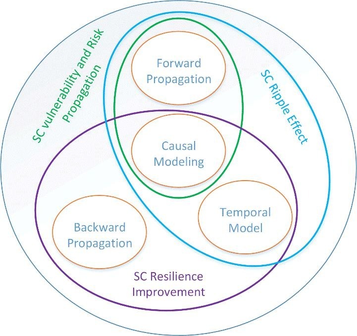
The interface of BN properties used for SC risk, resilience analysis, and ripple effect analysis.
The analysis of literature shows that the primary objective for the use of BNs is causal modelling, such as interdependency modelling between SC risks (e.g., Qazi et al., 2017, Qazi and Akhtar, 2018, Boutselis and McNaught, 2019), causal relationship modelling between disruptive events and resilience capacities (absorptive + adaptive + restorative) of SC entities (Hosseini and Barker, 201a, Hosseini and Barker, 2016b, Hosseini and Ivanov, 2019). Additionally, researchers used BNs to simulate and quantify the impact of natural disaster and operational risks on SC performance, particularly ripple effect modelling of supplier disruption using FP (Garvey et al., 2015, Hosseini et al., 2019b, Ojha et al., 2018, Yang and Liu, 2018). Lastly, BNs are used by researchers to find possible ways to improve SC resilience using BP analysis in a time dependent (temporal) model (Hosseini et al., 2016a, Hosseini et al., 2016b, Hosseini et al., 2019b, Hosseini et al., 2019a). The literature on BNs has been classified based on the main properties of BNs, causal, temporal, FP, and BP modelling, respectively, and are listed in Table 3 . Table 3 includes the papers that utilized the major features of BN. Combinations of BN features have been used in literature for SC vulnerability and risk propagation analysis, ripple effect modelling, and SC resilience improvement analysis.
Table 3.
Classification of SC risk and resilience studies based on the main features of BN.
| Article | Objective of article | Scope of article |
Main feature of BN used in the article |
Explanation | ||||
|---|---|---|---|---|---|---|---|---|
| SC risk | SC resilience | Causal modeling |
Forward Propagation |
Backward propagation |
Temporal model |
|||
| Hosseini and Barker (2016b) | Resilience supplier selection | ✓ | ✓ | ✓ | ✓ | BN is applied to model primary, green and Resilience criteria of supplier selection problem | ||
| Qazi et al. (2014) | SC risk assessment | ✓ | ✓ | ✓ | An integrated Game theory and BN approach is utilized to quantify SC risks | |||
| Wan et al. (2019) | Assessing maritime SC risks | ✓ | ✓ | BN is developed to quantify the risk of SC maritime risks | ||||
| Boutselis and McNaught (2019) | Spare demand forecasting | ✓ | ✓ | BN is used to forecast spare demand under disruption risk | ||||
| Hosseini et al. (2019d) | Ripple effect modeling of Supplier disruption | ✓ | ✓ | ✓ | ✓ | ✓ | DBN is used to model the ripple effect of supplier disruption | |
| Hosseini and Ivanov (2019) | SC resilience modeling with ripple effect consideration | ✓ | ✓ | ✓ | ✓ | Metrics are developed based on the application of BN to measure the vulnerability, recoverability and resilience of suppliers | ||
| Kumar Sharma and Sharma (2015) | SC risk assessment | ✓ | ✓ | BN is used to measure and evaluate SC risks | ||||
| Sharma and Routroy (2016) | SC information risk modeling | ✓ | ✓ | ✓ | BN is utilized to study the impact of Information breakdown and leakage on SC Revenue impact | |||
| SC resilience modeling | ✓ | ✓ | ✓ | SC resilience metric is proposed which is based on the forward propagation feature of BNs | ||||
| Qazi et al., 2017, Qazi and Akhtar, 2018 | SC network risk analysis | ✓ | ✓ | BN is used to analyze the SC network risks and causality relationship among risks | ||||
| Garvey et al. (2015) | SC risk propagation analysis | ✓ | ✓ | ✓ | A model based on BN is developed that measures the disruption propagation in SC networks | |||
| Ojha et al. (2018) | SC risk propagation of SC networks | ✓ | ✓ | ✓ | BN is used to model SC risk propagation | |||
| Yang and Liu (2018) | Vulnerability assessment of SC | ✓ | ✓ | BN is used to calculate the network Parameters of SC vulnerability | ||||
| Kaki et al. (2015) | Supplier disruption risk assessment | ✓ | ✓ | ✓ | BN is used to assess the SC network disruption by measuring the risk propagation of disrupted supplier | |||
| Hu et al. (2019) | Disruption risk analysis of SC | ✓ | ✓ | Effective disruptive mitigation policies are Suggested using BN to minimize disruption Risk in petroleum SC |
||||
| Qazi and Akhtar (2018) | SC risk modeling | ✓ | ✓ | ✓ | BN is used to model interdependency among SC risks and manage risk specific with respect to the risk appetite. | |||
| Rodgers and Singham (2019) | SC disruption modeling | ✓ | ✓ | BN is utilized to quantify the probability of Disruption in a clinical SC | ||||
| Lockamy and McCormack (2012) | Supplier risk analysis | ✓ | ✓ | ✓ | The revenue impact of supplier disruption Is evaluated using BN. | |||
| Rodger (2014) | SC risk modeling | ✓ | ✓ | ✓ | A fuzzy BN is proposed to predict supply chain backorder risk. | |||
These BN applications can provide a number of useful managerial insights. For example, managers can use BN to uncover associations between network structures and risk propagation. This would allow analyzing critical network elements leading to SC discontinuities and collapses through disruption propagation and modelling of interdependencies in SCs with consideration of state dynamics within SC nodes. Such an analysis can be applied to assessment of SC robustness and resilience to disruptions with the ripple effect considerations. Moreover, the BN make it possible to examine different disruption propagation mechanisms and identify disruption propagation scenarios of different severity for stress-testing of SC designs. This property can also be used to test the proneness of specific SC designs to disruption risk propagation.
7. Applying machine learning to BNs
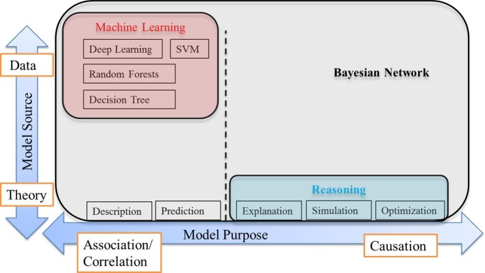
The structures of BN models that we have discussed so far are constructed solely based on expert elicitation. Many of BN models (e.g., Kumar Sharma and Sharma, 2015, Lockamy and McCormack, 2012) used expert knowledge to determine conditional probabilities for each node. In a real-life context, it is often unrealistic to expect precise probability estimations to be provided by experts (Constantinou, Fenton, & Neil, 2016). Besides, experts’ beliefs could be biased (Johnson, Tomlinson, Hawker, Granton, & Feldman, 2010). As such, recent literature extensively utilized learning techniques to forecast the values of some system-relevant parameters (Chen & Chao, 2020). Machine learning techniques, such as supervised and unsupervised learning algorithms, can be used to learn the structure (cause-effect relationship among nodes) of BNs. Recently, machine learning techniques have been reported to have their first applications to SC disruption risk analysis (Baryannis et al., 2019, Cavalcante, Frazzon, Forcellinia, & Ivanov, 2019, Mani et al., 2017, Shang et al., 2017, Ye et al., 2015, Zage et al., 2013). To better understand the application of machine learning in BNs, we created a map of analytic modelling and reasoning, as shown in Fig. 20 .
Fig. 20.
A map of analytic modelling for BN and machine learning (adapted from Conrady & Jouffe, 2018).
In Fig. 20, the x-axis represents the modelling purpose, which ranges from association/correlation to causation. Association/correlation is a model that explains the correlation between the variables, including description and prediction models such as neural networks. The causation models represent the causality of the variables, such as explanatory, simulation, and optimization models. The y-axis reflects the source of model, ranging from data to theory.
Traditionally, models have been built based on theory and estimated based on data (e.g., regression models). Today, due to the availability of big data and tools which make computation easier, machine learning algorithms can be used to create a BN model from data. Machine learning algorithms, as depicted in the upper left hand side of Fig. 20, are driven by data generally suitable for prediction. Unlike the machine learning algorithms, the structural equations models and regression are driven by theories that are used for prediction and or explanation. Considering the model source (y-axis), the structure of BNs can be built from theory (e.g., human learning, human intelligence, or can be developed based on data from machine learning, or a combination of both thereof).
Hereupon, the BN can be applied to the entire spectrum of model sources. In the context of SC resilience, the intra-causal relationships between SC risk factors (e.g., natural disasters, economic and political crises, transportation failures) and their causal influence on SC performance (e.g., cost, service level, lead time) can be understood based on data from machine learning (Ivanov and Dolgui, 2020). BNs can be used for causal reasoning and prediction purposes. Causal reasoning can be extensively used in the context of SC risk and resilience, e.g., if we wish to predict the consequences of specific disruption triggers (e.g., economic crises) on performance (e.g., delivery delay, loss of market share). The BN can facilitate this through causal reasoning by inputting evidence (setting the probability of economic crises to 100%) and updating the marginal probabilities of all unobserved variables. Causal reasoning in this case can tell us how much the probability of each consequence may vary if an economic crisis occurs.
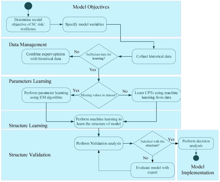
In summary, we propose a generic framework that integrates the BN with machine learning to model SC risk and resilience problems. This framework consists of five component steps, as illustrated in Fig. 21 .
Fig. 21.
General framework of a BN based on machine learning for SC risk and resilience problem analysis.
The steps in the framework shown in Fig. 21 are explained in detail below.
Step 1: Model objectives: The first step is to define model objectives. The primary objective in this study is to measure SC resilience and disruption risk. Once the model objective and the variables of BN models, such as disruption triggers, are specified, then consequences, etc., should be identified.
Step 2: Data management: The second step is to collect historical data. Historical data can be combined with expert knowledge if there is not sufficient data available. It is notable that the expert knowledge can be used for conditional probability elicitation, particularly when the risk is novel or very infrequent. Readers may refer to Wright and Ayton, 1987, Constantinou et al., 2016, and O’Hagan (2019) for more details about the integration of expert knowledge and historical data.
Step 3: Parameters and structure learning: This step, where the conditional probabilities (CPT) of BN variables and structure (causality) of the BN model are learned via machine learning algorithms, is the most important. It is notable that there might be missing values in the database. In such a case, an expectation–maximization (EM) algorithm can be used to estimate the CPT of the variable with the missing value.
Step 4: Model validation: Once the BN model is built, it is important to validate the structural design of the model. Different validation methods, such as cross-validation and sensitivity analysis, can be applied.
Step 5: Model implementation: The last step is to perform decision analysis to understand how the different types of disruptions could impact SC performance. Different types of “cause to effect” or forward propagation (FP) and “effect to cause” or backward propagation (BP) analyses can be performed to better understand the impact of contingency and mitigation strategies to improve SC resilience.
8. Conclusion and future research
BNs are a powerful methodology for managing risk assessment and decision-making subject to uncertainty. In the broad sense, BNs are probabilistic graphical models that possess unique methodical features to model dependencies in complex networks, such as forward and backward propagation (inference) of disruptions. BN techniques have been widely utilized by researchers to develop decision support systems in various sets of applications, including reliability engineering, system safety, medical diagnosis, equipment failure diagnosis, and demand forecasting.
The application of BNs in the field of SCRM is relatively new and allows obtaining novel insights which are difficult to examine with the help of other methods (Table 4 ). This study aims to introduce BNs into SC risk and resilience research. BNs have transitioned from an emerging topic to a growing research area in SC resilience and risk analysis. As a result, it is necessary to review existing literature to identify recent developments in this area and uncover potential directions for future research. Despite an increasing number of publications on BNs in research SC uncertainty, an extensive review on their application to SC risk and resilience is lacking. To address this gap, we analyzed research articles published in peer-reviewed academic journals published between 2007 and 2019 using network analysis, visualization-based scientometric analysis, and clustering analysis. Through this study, we contribute to literature by discussing the challenges of current research, and, more importantly, identifying and proposing directions for future research. The results of our survey show that further debate on the theory and application of BNs to SC resilience and risk management is a significant area of interest for both academics and practitioners. The applications of BNs and their conjunction with machine learning algorithms for solving big data SC problems under uncertainty and risks have also been discussed.
Table 4.
A comparison between different features of well-known methodologies for solving SC risk and resilience problems.
| Type of modeling |
Inference analysis |
Dependency modeling |
Type of relationship |
|||||
|---|---|---|---|---|---|---|---|---|
| Nonparametric | Parametric | Forward propagation | Backward propagation | Causation | Correlation | Linear | Nonlinear | |
| Bayesian Network | ✓ | ✓ | ✓ | ✓ | ✓ | ✓ | ✓ | ✓ |
| Linear regression | ✓ | ✓ | ✓ | ✓ | ✓ | |||
| Fault Tree | ✓ | ✓ | ||||||
| Markov Chain | ✓ | ✓ | ✓ | ✓ | ||||
| FMEA | ✓ | ✓ | ||||||
The results of our survey show that BNs are a suitable tool for SC risk and resilience problems, because they can easily capture causality and interdependency between SC risk sources, mitigation strategies, and consequences of risk. They can represent nonlinear relationships between variables in terms of conditional probability. BNs are particularly useful for modelling, measuring, and predicting SC resilience, because they can model the interdependency between drivers of mitigation and contingency disaster strategies. They can be used to simulate the impact of unforeseen disruptions on SC resilience through FP analysis. Through BP analysis, BNs can provide managerial insights concerning to what degree drivers of mitigation and contingency strategies must be improved to obtain a satisfactory level of resilience. Finally, given the increase in the availability of data and the number of SC companies seeking to utilize machine learning to increase profitability, the future development of BN models should be adapted through use of supervised and unsupervised learning algorithms.
Finally, we suggest potential research opportunities based on our analysis of the literature review and the gaps observed therein. The first future research direction relates to Dynamic Bayesian network (DBN) for SC resilience. The majority of current application of BNs for SC risk and resilience were static, and consequently they cannot capture the change in SC performance level (e.g., cost, service level, lead time). DBN is an appropriate methodology to dynamically simulate the vulnerability of SC entities. SC resilience can be measured as a function of its vulnerability and recoverability from disruption. The concept of resilience is dynamic and considers SC recovery from disrupted performance over time. Hence, DBN is a good choice for modelling the dynamicity feature of SC resilience. Future research opportunities can focus on developing DBN to quantify the resilience of SCs. Second, we point to analysis SC structural complexity. The vulnerability and recoverability of SCs depend on many factors such as their complexity and structure. It is more difficult to control and restrain the risk propagation in SCs with high level of complexity and interconnectedness. The future research attempts could focus on measuring and analyzing the propagation of risks on complex and interconnected networks. Finally, hybrid BN for SC risk and resilience represent a promising research area. BNs can be used in conjunction with other risk analysis approaches, such as FTD, FMEA, MCS, decision trees, Markov Chain, etc. One option is to develop an integration of continuous Markov chain model and BN to model the vulnerability and recoverability of SC entities. The transition probability between states of Markov chain model can be encoded using CPTs.
CRediT authorship contribution statement
Seyedmohsen Hosseini: Conceptualization, Methodology, Software, Visualization. Dmitry Ivanov: Writing - review & editing.
Declaration of Competing Interest
The authors declare that they have no known competing financial interests or personal relationships that could have appeared to influence the work reported in this paper.
References
- Athikulrat K., Rungreanganun V., Talabgaew S. Reliability assessment on member of supply chain based on SCOR performance and fault tree analysis. International Journal of Computer Science and Electronics Engineering. 2015;3(2):107–111. [Google Scholar]
- Bac Dang K., Windhorst W., Burkhard B., Muller F. A Bayesian belief network-based approach to link ecosystem functions with rice provisioning ecosystem services. Ecological Indicators. 2019;100:30–44. [Google Scholar]
- Baesens B., Verstraeten G., Van de Poel D., Egmont-Petersen M., Van Kenhove P., Vanthienen J. Bayesian network classifiers for identifying the slope of the customer lifecycle of long-life customers. European Journal of Operational Research. 2004;156(2):508–523. [Google Scholar]
- Baryannis G., Validi S., Dani S., Antoniou G. Supply chain risk management and artificial intelligence: State of the art and future research directions. International Journal of Production Research. 2019;57(7):2179–2202. [Google Scholar]
- Behzadi G., O’Sullivan M.J., Olsen T.L. On metrics for supply chain resilience. European Journal of Operational Research. 2020 doi: 10.1016/j.ejor.2020.04.040. [DOI] [Google Scholar]
- Blackhurst J., Dunn K.S., Craighead C.W. An empirically derived framework of global supply resiliency. Journal of Business Logistics. 2011;32(4):374–391. [Google Scholar]
- Blackhurst J., Wu T. Springer Publishing; New York: 2009. Managing supply chain risk and vulnerability: Tools and methods for supply chain decision makers. [Google Scholar]
- Bornmann L., Haunschild R., Hug S.E. Visualizing the context of citations referencing papers published by Eugene Grafield: A new type of keyword co-occurrence analysis. Scientometrics. 2018;114:427–437. doi: 10.1007/s11192-017-2591-8. [DOI] [PMC free article] [PubMed] [Google Scholar]
- Boutselis P., McNaught K. Using Bayesian networks to forecast spares demand from equipment failures in changing service logistics context. International Journal of Production Economics. 2019;209:325–333. [Google Scholar]
- Brandon-Jones E., Squire B., Autry C.W., Petersen K.J. A contingent resource-based perspective of supply chain resilience and robustness. Journal of Supply Chain Management. 2014;50(3):55–73. [Google Scholar]
- Buritica J., Tesfamariam S. Consequence-based framework for electric power providers using Bayesian belief network. International Journal of Electrical Power & Energy Systems. 2015;64:233–241. [Google Scholar]
- Cardoso S.R., Barbosa-Povoa A.P., Relvas S., Novais A.Q. Resilience metrics in the assessment of complex supply-chains performance operating under demand uncertainty. Omega. 2015;56:53–73. [Google Scholar]
- Cavalcante I.M., Frazzon E.M., Forcellinia F.A., Ivanov D. A supervised machine learning approach to data-driven simulation of resilient supplier selection in digital manufacturing. International Journal of Information Management. 2019;49:86–97. [Google Scholar]
- Chaudhuri A., Boer H., Taran Y. Supply chain integration, risk management and manufacturing flexibility. International Journal of Operations & Production Management. 2018;38(3):690–712. [Google Scholar]
- Chen B., Chao X. Dynamic inventory control with stockout substitution and demand learning. Management Science. 2020 doi: 10.1287/mnsc.2019.3474. [DOI] [Google Scholar]
- Computerworld. (2016). Japan earthquakes disrupt electronics supply chain. A major Sony camera sensor factory is offline after a series of quakes. https://www.computerworld.com/article/3057269/japan-earthquakes-disrupt-electronics-supply-chain.html.
- Conrady S., Jouffe L. 2nd ed. 2018. Bayesian networks & BayesiaLab: A practical introduction for researchers. [Google Scholar]
- Constantinou A., Fenton N., Neil M. Integrating expert knowledge with data in Bayesian networks: Preserving data-driven expectations when the expert variables remain unobserved. Expert Systems with Applications. 2016;56(1):197–208. doi: 10.1016/j.eswa.2016.02.050. [DOI] [PMC free article] [PubMed] [Google Scholar]
- Corani G., Magli C., Giusti A., Gianaroli L., Gambardella L.M. A Bayesian network model for predicting pregnancy after in vitro fertilization. Computers in Biology and Medicine. 2013;43(11):1783–1792. doi: 10.1016/j.compbiomed.2013.07.035. [DOI] [PubMed] [Google Scholar]
- Corman F., Kecman P. Stochastic prediction of train delays in real-time using Bayesian networks. Transportation Research-Part C. 2018;95:599–615. [Google Scholar]
- Craighead C.W., Blackhurst J., Rungtusanatham M.J., Handfield R.B. The severity of supply chain disruptions: Design characteristics and mitigation capabilities. Decision Science. 2007;38:131–156. [Google Scholar]
- Daemi T., Ebrahimi A., Fotuhi-Firuzabad M. Constructing the Bayesian network for components reliability importance ranking in composite power systems. International Journal of Electrical Power & Energy Systems. 2012;43(1):474–480. [Google Scholar]
- De Sa A., Pereira A., Pappa G. A customized classification algorithm for credit card fraud detection. Engineering Applications of Artificial Intelligence. 2018;72:21–29. [Google Scholar]
- Deleris L., Erhun F. Proceedings of the 2005 Winter Simulation Conference. 2005. Risk management in supply networks using Monte-Carlo simulation; pp. 1643–1649. [Google Scholar]
- Dolgui A., Ivanov D., Rozhkov M. Does the ripple effect influence the bullwhip effect? An integrated analysis of structural and operational dynamics in the supply chain. International Journal of Production Research. 2020;58(5):1285–1301. doi: 10.1080/00207543.2019.1627438. [DOI] [Google Scholar]
- Dolgui A., Ivanov D., Sokolov B. Ripple effect in the supply chain: An analysis and recent literature. International Journal of Production Research. 2018;56(1–2):414–430. [Google Scholar]
- Dolgui A., Ivanov D., Sokolov B. Reconfigurable supply chain: The X-Network. International Journal of Production Research. 2020;58(13):4138–4163. doi: 10.1080/00207543.2020.1774679. [DOI] [Google Scholar]
- Dubey R., Gunasekaran A., Childe S.J., Papadopoulos A., Blome C., Luo Z. Antecedents of resilient supply chains: An empirical study. IEEE Transactions on Engineering Management. 2019;66(1):8–19. [Google Scholar]
- Dury B., Valverde-Rebaza J., Moura M.-F., Andrade Lopes A. A survey of the applications of Bayesian networks in agriculture. Engineering Applications of Artificial Intelligence. 2017;65:29–42. [Google Scholar]
- Fahimnia B., Tang C.S., Davarzani H., Sarkis J. Quantitative models for managing supply chain risks: A review. European Journal of Operational Research. 2015;247:1–15. [Google Scholar]
- Fenton N., Neil M. CRC Press,Taylor & Francis Group; Boca Raton, FL: 2013. Risk assessment and decision analysis with Bayesian networks. [Google Scholar]
- Flores M., Nicholson A., Brunskill A., Korb K., Mascaro S. Incorporating expert knowledge when learning Bayesian network structure: A medical case study. Artificial Intelligence in Medicine. 2011;53(3):181–204. doi: 10.1016/j.artmed.2011.08.004. [DOI] [PubMed] [Google Scholar]
- Friedman N., Nachman I., Peer D. Proceedings of the fifteenth conference on uncertainty in artificial intelligence. Morgan Kufmann Publishers Inc.; 1999. Learning Bayesian network structure from massive datasets: the spare candidate algorithm; pp. 206–215. [Google Scholar]
- Garvey M.D., Carnovale S., Yeniyurt S. An analytical framework for supply network risk propagation: A Bayesian network approach. European Journal of Operational Research. 2015;243(2):618–627. [Google Scholar]
- Gemela J. Financial analysis using Bayesian networks. Applied Stochastic Models in Business Industry. 2001;17:57–67. doi: 10.1002/asmb.422. [DOI] [Google Scholar]
- Gupta R., Bruce-Konuah A., Howard A. Achieving energy resilience through smart storage of solar electricity at dwelling and community level. Energy and Building. 2019;195:1–15. [Google Scholar]
- Gupta S., Kim H.W. Linking structural equation modeling to Bayesian networks: Decision support for customer retention in virtual communities. European Journal of Operational Research. 2008;190(3):818–833. [Google Scholar]
- Haddawy P., Imrul Hassan A., Kasantikul R., Lawpoolsri S., Sa-angchai P., Kaewkungwal J., Singhasivanon P. Spatiotemporal Bayesian networks for malaria prediction. Artificial Intelligence in Medicine. 2018;84:127–138. doi: 10.1016/j.artmed.2017.12.002. [DOI] [PubMed] [Google Scholar]
- He J., Alavifard F., Ivanov D., Jahani H. A real-option approach to mitigate disruption risk in the supply chain. Omega: The International Journal of Management Science. 2018;88:133–149. doi: 10.1016/j.omega.2018.08.008. [DOI] [Google Scholar]
- Heckmann I., Comes T., Nickel S. A critical review on supply chain risk-definition, measure and modeling. Omega. 2015;52:119–132. [Google Scholar]
- Ho W., Zheng T., Yildiz H., Talluri S. Supply chain risk management: A literature review. International Journal of Production Research. 2015;53(16):5031–5069. [Google Scholar]
- Hong Z., Lee C.K.M., Zhang L. Procurement risk management under uncertainty: A review. Industrial Management & Data Systems. 2018;118(7):1547–1574. [Google Scholar]
- Hosseini S., Al Khaled A., Sarder M.D. A general framework for assessing system resilience using Bayesian networks: A case study of sulfuric acid manufacturer. Journal of Manufacturing Systems. 2016;41:211–227. [Google Scholar]
- Hosseini S., Barker K. A Bayesian network model for resilience-based supplier selection. International Journal of Production Economics. 2016;180:68–87. [Google Scholar]
- Hosseini S., Barker K. Modeling infrastructure resilience using Bayesian networks: A case study of inland waterway ports. Computers & Industrial Engineering. 2016;93:252–266. [Google Scholar]
- Hosseini S., Barker K., Ramirez-Marquez J.E. A review of definitions and measures of system resilience. Reliability Engineering & System Safety. 2016;145:47–61. [Google Scholar]
- Hosseini S., Ivanov D. A new resilience measure for supply networks with the ripple effect considerations: A Bayesian network approach. Annals of Operations Research. 2019 doi: 10.1007/s10479-019-03350-8. [DOI] [Google Scholar]
- Hosseini S., Ivanov D., Dolgui A. Ripple effect modeling of supplier disruption: Integrated Markov chain and dynamic Bayesian network approach. International Journal of Production Research. 2019 [Google Scholar]
- Hosseini S., Ivanov D., Dolgui A. Review of quantitative methods for supply chain resilience analysis. Transportation Research: Part E. 2019;125:285–307. [Google Scholar]
- Hosseini S., Morshedlou N., Ivanov D., Sarder M.D., Barker K., Al Khaled A. Resilient supplier selection and optimal order allocation under disruption risks. International Journal of Production Economics. 2019;213:124–137. [Google Scholar]
- Hu W., Li C., Ye C., Wang J., Wei W., Deng Y. Research progress on ecological models in the field of water eutrophication: CiteSpace analysis based data from the ISI web of science database. Ecological Modeling. 2019:410. [Google Scholar]
- Huck A., Monstadt J. Urban and infrastructure resilience: Diverging concepts and the need for cross-boundary learning. Environmental Science & Policy. 2019;100:211–220. [Google Scholar]
- Ivanov D. “A blessing in disguise” or “as if it wasn’t hard enough already”: Reciprocal and aggravate vulnerabilities in the supply chain. International Journal of Production Research. 2020;58(11):3252–3262. doi: 10.1080/00207543.2019.1634850. [DOI] [Google Scholar]
- Ivanov D. Viable Supply Chain Model: Integrating agility, resilience and sustainability perspectives – lessons from and thinking beyond the COVID-19 pandemic. Annals of Operations Research. 2020 doi: 10.1007/s10479-020-03640-6. [DOI] [PMC free article] [PubMed] [Google Scholar]
- Ivanov D. Predicting the impact of epidemic outbreaks on the global supply chains: A simulation-based analysis on the example of coronavirus (COVID-19/SARS-CoV-2) case. Transportation Research – Part E. 2020;136 doi: 10.1016/j.tre.2020.101922. 101922. [DOI] [PMC free article] [PubMed] [Google Scholar]
- Ivanov D., Dolgui A. A digital supply chain twin for managing the disruption risks and resilience in the era of Industry 4.0. Production Planning and Control. 2020 doi: 10.1080/09537287.2020.1768450. [DOI] [Google Scholar]
- Ivanov D., Dolgui A., Sokolov B. The impact of digital technology and Industry 4.0 on the ripple effect and supply chain risk analytics. International Journal of Production Research. 2019;57(3):829–846. [Google Scholar]
- Ivanov D., Dolgui A., Sokolov B., editors. Handbook of Ripple Effects in the Supply Chain. Springer; New York: 2019. [Google Scholar]
- Ivanov D., Dolgui A., Sokolov B., Ivanova M. Literature review on disruption recovery in the supply chain. International Journal of Production Research. 2017;55(20):6158–6174. [Google Scholar]
- Ivanov D., Sokolov B., Dolgui A. The Ripple effect in supply chains: Trade-off ‘efficiency-flexibility-resilience’ in disruption management. International Journal of Production Research. 2014;52(7):2154–2172. [Google Scholar]
- IvanovDolgui D. Low-Certainty-Need (LCN) supply chains: A new perspective in managing disruption risks and resilience. International Journal of Production Research. 2019;57(15–16):5119–5136. [Google Scholar]
- Johnson S., Tomlinson G., Hawker G., Granton J., Feldman B. Methods to elicit beliefs for Bayesian priors: A systematic review. Journal of Clinical Epidemiology. 2010;63(4):355–369. doi: 10.1016/j.jclinepi.2009.06.003. [DOI] [PubMed] [Google Scholar]
- Kaki A., Salo A., Talluri S. Disruptions in supply networks: A probabilistic risk assessment approach. Journal of Business Logistics. 2015;36(3):273–287. [Google Scholar]
- Kao H.Y., Haung C.H., Li H.L. Supply chain diagnostics with dynamic Bayesian networks. Computers & Industrial Engineering. 2005;49(2):339–347. [Google Scholar]
- Kim Y., Chen Y., Linderman K. Supply network distribution and resilience: A network structural perspective. Journal of Operations Management. 2015;33:43–59. [Google Scholar]
- Kita E., Harada M., Mizuno T. Application of Bayesian network to stock price prediction. Artificial Intelligence Research. 2012;1(2):171–184. [Google Scholar]
- Koller D., Friedman N. 1st ed. The MIT Press; Cambridge, Massachusetts: 2012. Probabilistic graphical models: Principles and techniques (adaptive computation and machine learning series) [Google Scholar]
- Kontkanen P., Myllymaki P., Silander T., Tirri H. Proceedings of the Sixth International Workshop on Artificial Intelligence and Statistics, Ft. Lauderdale. 1997. Comparing predictive inference methods for discrete domains; pp. 311–318. [Google Scholar]
- Kumar Sharma S., Bhat A. Supply chain risks: Development of model and empirical evidence. International Journal of Applied Management Science. 2014;6(1):45–64. [Google Scholar]
- Kumar Sharma S., Sharma S. Developing a Bayesian network model for supply chain risk assessment. Supply Chain Forum: An international Journal. 2015;16(4) [Google Scholar]
- Labatut V., Pastor J., Ruff S., Demonet J., Celsis P. Cerebral modeling and dynamic Bayesian networks. Artificial Intelligence in Medicine. 2004;30(2):119–139. doi: 10.1016/s0933-3657(03)00042-3. [DOI] [PubMed] [Google Scholar]
- Lau C.L., Mayfields H.J., Lowry J.H., Watson C.H., Kama M., Nilles E.J., Smith C.S. Unravelling infectious disease eco-epidemiology using Bayesian networks and scenario analysis: A case study of leptospirosis in Fiji. Environmental Modeling & Software. 2017;97:271–286. [Google Scholar]
- Lazkano E., Sierra B., Astigarraga A., Martinez-Otzeta M. On the use of Bayesian networks to develop behaviours for mobile robots. Robotics and Autonomous Systems. 2007;55(3):253–265. [Google Scholar]
- Li X., Chandra C. A knowledge integration framework for complex network management. Industrial Management & Data Systems. 2007;107(8):1089–1109. [Google Scholar]
- Li S., Zeng W. Risk analysis for the supplier selection problem using failure modes and effects analysis (FMEA) Journal of Intelligence Manufacturing. 2016;27(6):1309–1321. [Google Scholar]
- Liu X. Proceedings of the six international conference on management science and engineering management. 2012. Analysis on supply chain risk factors based on structural equation model; pp. 829–837. [Google Scholar]
- Liu Z., Yin Y., Liu W., Dunford M. Visualizing the intellectual structure and evolution of innovation systems research: A bibliometric analysis. Scientometric. 2015;103(1):135–158. [Google Scholar]
- Livescience (2013). Two years later: lessons from Japan’s Tohoku earthquake. https://www.livescience.com/27776-tohoku-two-years-later-geology.html.
- Lockamy A., McCormack K. Modeling supplier risks using Bayesian networks. Industrial Management & Data Systems. 2012;11(2):313–333. [Google Scholar]
- Macdonald J.R., Zobel C.W., Melnyk S.A., Griffis S.E. Supply chain risk and resilience: Theory building through structured experiments and simulation. International Journal of Production Research. 2018;56(12):4337–4355. [Google Scholar]
- Mani V., Delgado C., Hazen B., Patel P. Mitigating supply chain risk via sustainability using big data analytics: Evidence from the manufacturing supply chain. Sustainability. 2017;9(4) [Google Scholar]
- Mishra D., Dwivedi Y., Rana N., Hassini E. Evolution of supply chain ripple effect: A bibliometric and meta-analytic view of the constructs. International Journal of Production Research. 2019 in press. [Google Scholar]
- Mola M., Feofilovs M., Romagnoli F. Energy resilience: Research trends at urban, municipal and country levels. Energy Procedia. 2018;147:104–113. [Google Scholar]
- Munya P., Ntuen C.A., Park E.H., Kim J.H. A Bayesian abduction model for extracting the most probable evidence to support sensemaking. International Journal of Artificial Intelligence & Applications. 2015;6(1):1–20. doi: 10.5121/ijaia.2015.6101. [DOI] [Google Scholar]
- Myllymaki P., Silander T., Tirri H., Uronen P. B-Course: A web-based tool for Bayesian and causal analysis. International Journal of Artificial Intelligence Tools. 2002;11(3):369–387. [Google Scholar]
- Nature (2011). Japan’s tsunami warning system retreats. https://www.nature.com/news/2011/110811/full/news.2011.477.html.
- Nepal B., Prakash Yadav O. Bayesian belief network-based framework for sourcing risk analysis during supplier selection. International Journal of Production Research. 2015;53(20):6114–6135. [Google Scholar]
- O’Hagan A. Expert knowledge elicitation: Subjective but scientific. The American Statistician. 2019;73(1):69–81. [Google Scholar]
- Ojha R., Ghadge A., Kumar Tiwari M., Bititci U. Bayesian network modeling for supply chain risk propagation. International Journal of Production Research. 2018;17:5795–5819. [Google Scholar]
- Pearl J. Morgan Kaufman; San Mateo, CA: 1988. Probabilistic reasoning in intelligence systems. [Google Scholar]
- Petousis P., Han S., Aberle D., Bui A. Prediction of lung cancer incidence on the low-dose computed tomography arm of the national lung screening trial: A dynamic Bayesian network. Artificial Intelligence in Medicine. 2016;72:42–55. doi: 10.1016/j.artmed.2016.07.001. [DOI] [PMC free article] [PubMed] [Google Scholar]
- Pettit T.J., Croxton K.L., Fiksel J. The evolution of resilience in supply chain management: A retrospective on ensuring supply chain resilience. Journal of Business Logistics. 2019;40(1):56–65. [Google Scholar]
- Pollino, C.A., Handerson, C. (2010). Bayesian networks: A guide for their application in natural resource management and policy. Technical Report No. 14. Landscape Logic.
- Pournader M., Kach A., Talluri S. A Review of the existing and emerging topics in supply chain risk management literature. Decision Sciences. 2020 doi: 10.1111/deci.12470. [DOI] [PMC free article] [PubMed] [Google Scholar]
- Qazi A., Akhtar P. Risk matrix driven supply chain risk management: Adapting risk matrix based tools to modeling interdependent risks and risk appetite. Computers & Industrial Engineering. 2018 doi: 10.1016/j.cie.2018.08.002. [DOI] [Google Scholar]
- Qazi A., Dickson A., Quigley J., Gaudenzi B. Supply chain risk network management: A Bayesian belief network and expected utility based approach for managing supply chain risks. International Journal of Production Economics. 2018;196:24–42. [Google Scholar]
- Qazi, A., Quigley, J., Dickson, A. (2014). A novel framework for quantification of supply chain risks. 4th Student Conference on Operational Research (SCOR’14), Open Access Series in Informatics (pp. 1–15).
- Qazi A., Quigley J., Dickson A., Ekici S. Exploring dependency based probabilistic supply chain risk measures for prioritizing interdependent risks and strategies. European Journal of Operational Research. 2017;259(1):189–204. [Google Scholar]
- Rajesh R. Measuring the barriers to resilience in manufacturing supply chains using Grey Clustering and VIKOR approaches. Measurement. 2018;126:259–273. [Google Scholar]
- Reuters. (2016). Toyota, other major Japanese firms hit by quake damage, supply disruptions.
- Rodger J.A. Application of a fuzzy feasibility Bayesian probabilistic estimation of supply chain backorder aging, unfilled backorders, and customer wait time using stochastic simulation with Markov blankets. Expert Systems with Applications. 2014;41(16):7005–7022. [Google Scholar]
- Rodgers M., Singham D. A framework for assessing disruptions in a clinical supply chain using Bayesian belief networks. Journal of Pharmaceutical innovation. 2019:1–15. [Google Scholar]
- Sawik T. 2nd ed. Springer; New York: 2020. Supply chain disruption management. ISBN 978-3-030-44813-4. [Google Scholar]
- Scheibe K.P., Blackhurst J. Supply chain disruption propagation: A systemic risk and normal accident theory perspective. International Journal of Production Research. 2018;56(1–2):43–59. [Google Scholar]
- Shang Y., Dunson D., Song J.-S. Exploiting big data in logistics risk assessment via Bayesian nonparametrics. Operations Research. 2017;65(6):1574–1588. [Google Scholar]
- Sharma S., Routroy S. Modeling information risk in supply chain using Bayesian networks. Journal of Enterprise Information Management. 2016;29(2):238–254. [Google Scholar]
- Shevtshenko E., Wang Y. Decision support under uncertainties based on robust Bayesian networks in reverse logistics management. International Journal of Computer Applications in Technology. 2009;36(3/4):247–258. [Google Scholar]
- Sodhi M.S., Tang C.S. Wiley encyclopedia of operations research and management science. John Wiley & Sons Inc; 2010. Supply chain risk management. [Google Scholar]
- Sreedevi R., Saranga H. Uncertainty and supply chain risk: The moderating role of supply chain flexibility in risk mitigation. International Journal of Production Economics. 2017;193:332–342. [Google Scholar]
- Srikanta Routroy S.S. Modelinfg information risk in supply chain using Bayesian networks. Journal of Enterprise Information Management. 2016;29(2):125–139. [Google Scholar]
- Tavana M., Abtahi A., Di Caprio D., Poortarigh M. An artificial neural network and Bayesian network model for liquidity risk assessment in banking. Neurocomputing. 2018;275:2525–2554. [Google Scholar]
- Teasley R., Bemley J., Davis L.B., Erera A., Chang Y. A Markov chain model for quantifying consumer risk in food supply chains. Health Systems. 2016;5(2):149–161. [Google Scholar]
- Uusitalo L. Advantages and challenges of Bayesian networks in environmental modeling. Ecological Modeling. 2007;203:312–318. [Google Scholar]
- Van Eck, N.J., Waltman, L. (2014). Citation-based clustering of publications using CitNetExplorer and VOSviewer. https://arxiv.org/ftp/arxiv/papers/1702/1702.03411.pdf. [DOI] [PMC free article] [PubMed]
- Wan C., Yan X., Qu Z., Yang Z. An advanced fuzzy Bayesian-based FMEA approach for assessing maritime supply chain risks. Transportation Research-Part E. 2019;125:222–240. [Google Scholar]
- Wang K., Chen J., Wang K. Medical expenditure estimation by Bayesian network for lung cancer patients at different severity stages. Computers in Biology and Medicine. 2019;106:97–105. doi: 10.1016/j.compbiomed.2019.01.015. [DOI] [PubMed] [Google Scholar]
- Wright G., Ayton P. Eliciting and modeling expert knowledge. Decision Support Systems. 1987;3(1):13–26. [Google Scholar]
- Wu J. Quantifying flexibility contracts under Bayesian updating. Computers & Operations Research. 2005;32(5):1267–1288. [Google Scholar]
- Xiang C., Wang Y., Liu H. A scientometric review on nonpoint source pollution research. Ecological Engineering. 2017;99:400–408. [Google Scholar]
- Yang J., Liu H. Research of vulnerability for fresh agricultural-food supply chain based on Bayesian network. Mathematical Problems in Engineering. 2018 doi: 10.1155/2018/6874013. [DOI] [Google Scholar]
- Ye S., Xiao Z., Zhu G. Identification of supply chain disruptions with economic performance of firms using multi-category support vector machines. International Journal of Production Research. 2015;53(10):3086–3103. [Google Scholar]
- Yoon J., Talluri S., Yildiz H., Ho W. Models for supplier selection and risk mitigation: A holistic approach. International Journal of Production Research. 2018;56(10):3636–3661. [Google Scholar]
- Yu L., Wang G., Marcouiller D.W. A scientometric review of pro-poor tourism research: Visualization and analysis. Tourism Management Perspective. 2019;30:75–88. [Google Scholar]
- Zage, D., K. Glass, R. Colbaugh (2013). Improving supply chain security using big data. In: 2013 IEEE International Conference on Intelligence and Security Informatics: Big Data, Emergent Threats, and Decision-Making in Security Informatics, IEEE, Seattle, WA, USA, 2013 (pp. 254–259).
- Zhao K., Zuo Z., Blackhurst J.V. Modelling supply chain adaptation for disruptions: An empirically grounded complex adaptive systems approach. Journal of Operations Management. 2019;65(2):190–212. [Google Scholar]
- Zhong H., Nof S. Springer; New York: 2020. Dynamic lines of collaboration. Disruption handling & control. 978-3-030-34462-7. [Google Scholar]
- Zhong B., Wu H., Li H., Sepasgozar S., Luo H., He L. A scientometric analysis and critical review of construction related ontology research. Automation in Construction. 2019;101:17–31. [Google Scholar]
- Zsidisin G.A., Ritchie R. Springer Publishing; New York: 2010. Supply chain risk: A handbook of assessment, management, and performance. [Google Scholar]


