Comprehensive identification and isolation policies have effectively suppressed the spread of COVID-19

Abstract

The outbreak of COVID-19 has caused severe life and economic damage worldwide. Since the absence of medical resources or targeted therapeutics, systemic containment policies have been prioritized but some critics query what extent can they mitigate this pandemic. We construct a fine-grained transmission dynamics model to forecast the crucial information of public concern, therein using dynamical coefficients to quantify the impact of the implement schedule and intensity of the containment policies on the spread of epidemic. Statistical evidences show the comprehensive identification and quarantine policies eminently contributed to reduce casualties during the phase of a dramatic increase in diagnosed cases in Wuhan and postponing or weakening such policies would undoubtedly exacerbate the epidemic. Hence we suggest that governments should swiftly execute the forceful public health interventions in the initial stage until the pandemic is blocked.

1. Introduction

Pneumonia caused by COVID-19 has evolved a worldwide pandemic for which humans have paid more than 8 million infections and 431 thousand deaths as of June 16th, 2020 [1] but there are still billions of lives threatened [2], [3], [4]. The transmission of the COVID-19 virus is confirmed through respiratory droplet [5] and has super infectivity beyond SARS and MERS [6] which can even overwhelm countries with advanced medical facilities and therapeutics. Laboratory experiments have proved that SARS-CoV-2 could survive temperatures of 56 ^∘C for more than 30 min [7] and the experiences from tropical regions illustrate that COVID-19 still has transmission capacity under the hydrothermal circumstance [8], [9]. Moreover, the incubation period of COVID-19 is relatively short (5.1 days average) implying that it quickly onset after infection and the infectors would present the corresponding clinical symptoms such as fever, cough, and fatigue [10], [11]. Recently, the revised data released by Chinese health authorities definitely delivered that the case fatality rate (CFI) of COVID-19 were seriously underestimated because the omission and false positive in the early stage of the pandemic. Given the current situation of the limited pharmaceutical treatments and the unavailable targeted vaccines [12], the public health interventions have been demonstrated as the most functional precautions in many countries [13], [14], especially contributing to block the epidemic in Wuhan [15], [16], [17], [18].

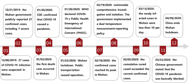
On Jan. 23th 2020, Chinese authorities imposed a lockdown in Wuhan since the suspected and diagnosed cases exceed 2000 which triggers public health emergency response in Hubei Province (Fig. 1 ). The containment efforts including school closures, transports bans and workplace shutdowns were announced to limit the spread of virus. Nevertheless, the epidemic entered the exponential period unstoppably from Feb. 2nd [19], [20] and caused global panic. The successive delivery of the shelter hospitals indicated Wuhan had the sufficient negative-pressure wards to isolate and treat symptomatic patients. Meanwhile, people strictly followed the ordinances concerning social distancing, quarantine and careful hand and respiratory hygiene, subsequently wearing personal protective equipments (PPE) [21], isolating themselves at home, and recording their temperature each day. The communities adopted a comprehensive identification strategy to detect the suspected cases and reported their trace while hiding their private information [22] resulting in a sub-exponential growth of the infection curve until a peak of 38,020 on Feb. 18th [23]. Despite there was a ethical controversy about whether suspicious individuals should be mandatorily isolated from social networks, the experiences from Wuhan supported this policy had effectively cut off the transmission channels of COVID-19 and compel the pandemic to a mitigation stage. In post-pandemic phase [24], Wuhan continued to distribute disinfectors throughout the region including ventilation duct, water pipe, and urban sewers where COVID-19 was sampled in Paris [25] and the central China government stated the pandemic was basically blocked on Mar. 23th. Ultimately, after paying 4632 deaths nationwide and incalculable economic cost, China ended its 76-day lockdown of Wuhan, but the relative restrictions still remained in place.

Fig. 1.

The diagram of the tendency of COVID-19 pandemic and the announcement timeline of the government containment policies.

However, the transmission dynamics observed in different continents and zones are markedly heterogeneous consulting time series data released by public health authorities [26], [27], [28], [29]. The fundamental reasons are that the fluctuation of the objective physical environments and the implementation intensity and duration of the containments policies restricted by public opinion, both presenting challenges to build the dynamic model to forecast the tendency of the pandemic. Furthermore, the CFI and recovery rate varies as well with respect to different phases since the gradual enrichment of healthcare experiences and capacities. Hence we propose dynamical coefficients to quantify the variation of infectivity, intervention policies, and vital dynamics to adjust the social responses to the pandemic in our model. Functionally, tuning the boundaries or the curvature of a dynamical coefficient can subtly regulate the corresponding containment effort and further observe its impact on the infection curve. We then simulate the results about advancing or postponing, reinforcing or weakening relevant policies and conclude that the output curves are sensitive to amplitude or period modulations of the dynamical coefficients. Through mapping the containment policies into measurable interval coefficients to observe their influence on the epidemic, the results of our model introduce statistical evidences that such policies can effectively suppress or even block the outbreak of COVID-19.

2. Preliminary

The classical SEIR (Susceptible - Exposed - Infectious - Recovered) model straightforwardly divides the population into four states and using ordinary differential equation (ODE) to reflect their transition in an epidemic [30]. The susceptible group generally refers to individuals who lack immunity to a virus on social networks and the infectious rate β′ determines how likely a susceptible person would be infected in the community. During the incubation duration, the individuals who are infected but not yet infectious are classified as the exposed cluster. The incubation rate σ′ represents the probability of transition from an exposed to an infectious individual. Considering the regional care capacity, only a fraction of γ′ (recovery rate) infectious patients would be cured each day. We assume they are noninfectious and would not be secondary infected after discharging from hospitals based on the current research evidences [31]. Therefore, the ODEs of SEIR model are:

$$\begin{array}{cc}& {\displaystyle \frac{dS}{dt}=-\frac{{\beta }^{\prime }SI}{N}}\hfill \\ & {\displaystyle \frac{dE}{dt}=-\frac{{\beta }^{\prime }SI}{N}-{\sigma }^{\prime }E}\hfill \\ & {\displaystyle \frac{dI}{dt}={\sigma }^{\prime }E-{\gamma }^{\prime }I}\hfill \\ & {\displaystyle \frac{dR}{dt}={\gamma }^{\prime }I}\hfill \end{array}$$ (1)

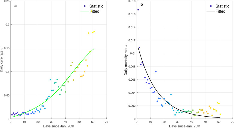
There are several deficiencies when using SEIR model to describe the transmission dynamics of COVID-19 pandemic. For examples, many crucial factors such as morality rate, public health intervention, migration of population, diagnosis capacity, are ignored in SEIR and therefore it can be regarded as a natural transmission model under ideal conditions. Moreover, SEIR inappropriately defines the constant infectious rate β′ and recovery rate γ′ during the entire spread period. In practice, the statistic evidences collected in Wuhan (Fig. 2 ) show that the daily recovery rate has gradually increased to a peak and the daily morality rate has gradually decreased to 0 with the improvement of healthcare capacity. Furthermore, the infectiousness of COVID-19 obviously decays as the implement of containment policies [31].

Fig. 2.

The daily recovery rate and morality rate of COVID-19 pandemic in Wuhan. The dots denote the statistical data released by NHC and the curves denote the fitted data based on arctangent and exponential functions. a The curve of daily cure rate. The daily cure rate is calculated from the ratio of the number of daily cured cases to the existing infected cases. b The curve of daily morality rate. The daily morality rate is calculated from the ratio of the number of daily deaths to the existing infected cases.

3. Modeling transmission dynamics of COVID-19

3.1. ICRD model

From the traces and cases information of patients released by the Wuhan government and National Health Commission (NHC), most individuals were infected from symptomatic or pre-symptomatic transmission, especially during the phase of exponential and sub-exponential growth, whereas the persons who were infected through asymptomatic or environmental transmission accounted for a considerable fraction of infectors as well. In practice, the boundaries of these four transmissions are ambiguous such as a asymptomatic might subsequently develop into a symptomatic. Therefore, we generally classify the people who have infectiousness as the infected cluster and assume the non-isolated infected individuals are the main propagating sources on social networks. We divide the states of the population into 4 categories: (H)ealthy, (I)nfected, (R)ecovered and (D)eceased (Fig. 3 ). More granular, the infected group I consists of the confirmed C and unconfirmed $I-C$ and therein the confirmed individuals C are either isolated βC (β is the isolation rate) or non-isolated $(1-\beta )C$. Then the transmission dynamics of virus can be fully described by the following ODEs with respect to time t (namely ICRD model):

$$\begin{array}{cc}& \frac{dI}{dt}=\dot{I}=\alpha (I-\beta C)(1-{\left(\frac{I}{N}\right)}^{{\gamma }^{-1}})-(\sigma +\kappa )C-(\delta +\mu )(I-C)\hfill \\ & \frac{dC}{dt}=\dot{C}=\eta (I-C)-\sigma C-\kappa C\hfill \\ & \frac{dR}{dt}=\dot{R}=\sigma C+\delta (I-C)\hfill \\ & \frac{dD}{dt}=\dot{D}=\kappa C+\mu (I-C)\hfill \end{array}$$ (2)

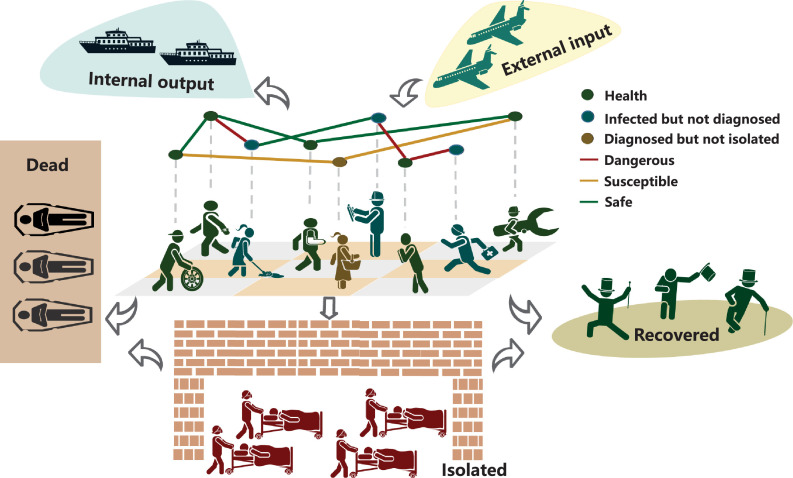
Fig. 3.

Transmission mechanism of COVID-19 on social networks. The group of infected but non-isolated (blue and yellow nodes) is the main propagating source of virus through physical contacts (droplet), especially over the incubation period [32], [33]. The infected patients would die or produce antibodies without treatment but undoubtedly the herd immunity would take a long time to achieve and uncountable individuals would lose their lives in this process. Therefore, the diagnosed patients should be isolated from social networks to cut off the transmission links (yellow edges). Due to the red edges are more dangerous for the exposed persons, the comprehensive identification policy for all people and the nucleic acid testing strategy for symptomatic patients should be taken to remove their connections with others. Meanwhile, some carrier would migrate to other place through the global transportation networks. The experiences from China demonstrated that the external input is the largest threat in the post-transmission period [34]. (For interpretation of the references to colour in this figure legend, the reader is referred to the web version of this article.)

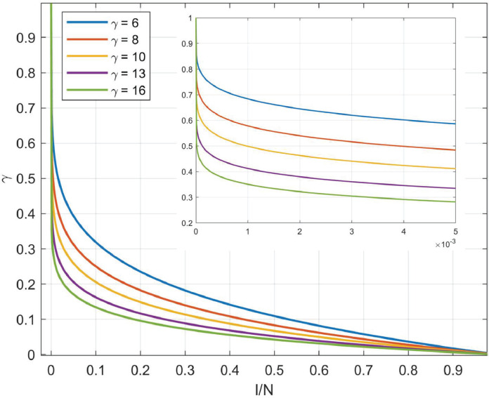
If the system is closed, implying the targeted area is locked as soon as identifying the infected case, the healthy population will be $H=N-I-R-D$. Otherwise, if people can move freely when the outbreak occurs, $H=N\left(t\right)-I-R-D,$ indicating the total population changes over time. The infected but non-isolated group $I-\beta C$ has the fierce infectiousness since they not only are the virus carriers but can randomly walk on social networks. The average number of secondary infections an infected would induce over the period from infected to isolated T (transmission is terminated) is defined as the basic reproduction number R ₀. The infectiousness intensity in a unit period is $\alpha =R_0/T$ and the new increase of infected individuals thereby are $\alpha (I-\beta C)$. Apparently, α is inversely proportional to social distancing, determining the increment of infected cases each day and tuning α could capture the effect of isolation policies subtly. Nevertheless, one person would be repeatedly secondarily infected with high probability when the infection density in the community reaches a critical level and above statistical value significantly greater than the true value. We then present a harmonic function $(1-{(I/N)}^{{\gamma }^{-1}})$ (Fig. 4 ) to tackle the redundancy counting dilemma, in which N represents the community population and γ denotes the harmonic coefficient. $\alpha (1-{(I/N)}^{{\gamma }^{-1}})$ shows the infectivity of an individual would degrade as the group density of infection increases. Meanwhile, there would be a proportion of infectors who recover (cured after treatment σC or spontaneous recovery κC) or die (die with treatment $\delta (I-C)$ or without treatment $\mu (I-C)$) in one unit statistical period, where σ, κ, δ, μ are daily cure rate, incurable mortality rate, natural recovery rate, and non-treatment mortality rate, respectively. Hence $\dot{I}$ quantifies the aggregate incremental cases of infection after removing the recovered and dead population. Limiting to the objective medical testing ability of laboratories, only a fraction of η suspected cases could receive diagnosis within the unit statistical period (η is the algebraic mapping of identification policy), then the gradient of confirmed cases $\dot{C}$ equals to the difference between the newly positive diagnosed cases $\eta (I-C)$ and the dead or recovered cases $(\sigma +\kappa )C$. Ultimately, we could deduce the daily increase of recovered or dead cases integrating the recovery ratio σ, δ and mortality κ, μ with the infected population. Furthermore, some other key information can be indirectly calculated based on ICRD. For example, the total daily increment of the infected but unconfirmed group is:

$$\frac{d(I-C)}{dt}=\alpha (I-\beta C)(1-{\left(\frac{I}{N}\right)}^{{\gamma }^{-1}})-\eta (I-C)-(\delta +\mu )(I-C)$$ (3)

the cumulative infectors at period t* are:

$${\int }_0^{t^{*}}\frac{dI}{dt}+(\sigma +\kappa )C+(\delta +\mu )(I-C)dt=\sum _{\tau =0}^{t^{*}}\frac{dI}{dt}{|}_{\tau }+(\sigma +\kappa )C_{\tau }+(\delta +\mu )(I_{\tau }-C_{\tau })$$ (4)

where we assume that the unit statistic time is one day. Similarly, the cumulative confirmed cases are:

$${\int }_0^{t^{*}}\frac{dC}{dt}+(\sigma +\kappa )Cdt=\sum _{t=0}^{t^{*}}\frac{dC}{dt}{|}_{\tau }+(\sigma +\kappa )C_{\tau }$$ (5)

From Fig. 3, there may be some output ξ(t) and input infection cases χ(t) each day and then $\dot{I}$ (Eq. (2)) becomes:

$$\begin{array}{ccc}\hfill \frac{dI}{dt}& =& \alpha (I-\beta C)(1-{\left(\frac{I}{N}\right)}^{{\gamma }^{-1}})-(\sigma +\kappa )C-(\delta +\mu )(I-C)\hfill \\ & & -\xi \left(t\right)+\chi \left(t\right)\hfill \end{array}$$ (6)

Fig. 4.

The curves of the harmonic function under different harmonic coefficients. The harmonic function is presented to tackle the redundancy count of infectors and controlled by the harmonic coefficient γ which is determined by the population density and natural environment of the targeted region. The horizontal axis denotes the ratio of the infected cases to the total population.

3.2. Using dynamical coefficients to quantify the identification and isolation policies

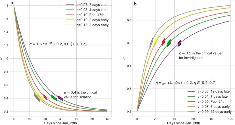
Before we have discussed that β and η map the impact of the isolation and identification policies on a pandemic in ICRD model, respectively. The constant coefficients in Eq. (2) assume that the containment efforts or the physicochemical properties of coronavirus remain permanent in long-term transmission, and undoubtedly it is counterintuitive. In fact, the governments tend to adopt more compulsive policies as the dramatic increase of death cases, residents choose isolate themselves spontaneously with more publicity on negative news, and the testing and diagnosis techniques would be visibly improved after the deeply studying of the virus’s properties. Hence the measures and intensity of the society to fight the pandemic change in different phases. For instance, initially, due to the lack of awareness of the virus, people are reluctant to maintain social distancing with others (R ₀ and α are relatively large), so the virus has explosive infectivity at this stage. Subsequently, with the exponential increase of infected cases, the government would announce voluntary or compulsive isolation policies to reduce α until it remains a low level (Fig. 5 a). Furthermore, many susceptible patients cannot be diagnosed because of the limited medical resources in the preliminary stage. However, the promotion of the testing techniques and the enhancement of the identification policies (η rises) would strongly reverse this situation in the successive stages. Therefore, we introduce the dynamical coefficients to simulate the transformation of propagation:

$$\alpha =a*e^{-bt}+c$$ (7)

$$\eta =u*\arctan \left(vt\right)+w$$ (8)

Fig. 5 illustrates the curves of dynamical α and η, and it is clear that the parameters a, c (or u, v) determine the boundaries of α (or η) which catch the intensity scope of the isolation (investigation) policies and b (or v) is a critic to evaluate the response time of these policies, both regulating the tendency of epidemic.

Fig. 5.

Mathematical representations of dynamical coefficients with respect to isolation policy and identification policies respectively. (a) tuning the parameter b of α can subtly regulate the implement schedule of isolation policy. We choose $\alpha =0.4$ as the critical value for daily isolation rate at which this policy is fully implemented. The practical isolation policy curve $b=0.10$ (Feb. 17th) is selected as the baseline to compare results calculated by advancing or postponing of this policy. The boundaries of α ∈ [1.8, 0.2] are determined by the basic reproduction number R₀ and the duration from infected to infected. (b) tuning the parameter v of η can reflect the rate of community identification for the infected but undiagnosed patients. We choose $\eta =0.5$ as the threshold of daily identification rate and $v=0.05$ (Feb. 24th) as the baseline to compare the impact of the implement schedule of identification policy to the pandemic trend. The boundaries of η ∈ [0.2, 0.7] are determined by the testing ability of laboratories.

3.3. The criterion to determine the dynamical coefficients

In the above, we show that tuning dynamical coefficients can precisely regulate the implement schedule and intensity of the corresponding policies. Furthermore, the parameters space of these dynamical coefficients is also restricted in mathematic. For example, to ensure the convergence and non-negativity of the output curves, the ODEs should satisfy the following constrains:

$$\begin{array}{ccc}\hfill I\left(t\right)& \ge & 0,\underset{t\to \infty }{\lim }\frac{dI}{dt}=0\hfill \\ \hfill C\left(t\right)& \ge & 0,\underset{t\to \infty }{\lim }\frac{dC}{dt}=0\hfill \\ \hfill R\left(t\right)& \ge & 0,\underset{t\to \infty }{\lim }\frac{dR}{dt}=0\hfill \\ \hfill D\left(t\right)& \ge & 0,\underset{t\to \infty }{\lim }\frac{dD}{dt}=0\hfill \end{array}$$

This implies that the nonlinear system constituted by ICRD is stable and has only one equilibrium $\theta =[I,C,R,D]=[0,0,cons{t}_1,cons{t}_2],$ where const denotes the positive constant. The Hesse matrix of Eq. (2) is:

$$\begin{array}{ccc}\hfill H& =& {\left(\begin{array}{cccc}\partial \dot{I}/\partial I& \partial \dot{I}/\partial C& \partial \dot{I}/\partial C& \partial \dot{I}/\partial D\\ \partial \dot{C}/\partial I& \partial \dot{C}/\partial C& \partial \dot{C}/\partial C& \partial \dot{C}/\partial D\\ \partial \dot{R}/\partial I& \partial \dot{R}/\partial C& \partial \dot{R}/\partial C& \partial \dot{R}/\partial D\\ \partial \dot{D}/\partial I& \partial \dot{D}/\partial C& \partial \dot{D}/\partial C& \partial \dot{D}/\partial D\end{array}\right)}_{\theta }\hfill \\ & =& \left(\begin{array}{cccc}\alpha -\delta +\mu & -\alpha \beta -\sigma -\kappa +\delta +\mu & 0& 0\\ \eta & -\eta -\sigma -\kappa & 0& 0\\ \delta & \sigma -\delta & 0& 0\\ \mu & \kappa -\mu & 0& 0\end{array}\right)\hfill \end{array}$$

[λ ₁, λ ₂, λ ₃, λ ₄] are the eigenvalues of H. To ensure the stability of the system at the equilibrium θ, they should satisfy ${\lambda }_i\le 0,\forall i=1,2,3,4$ [35].

4. Results

In our experiments, the default coefficients of SEIR are shown in Table 1 and the default static and dynamical coefficients are shown in Table 2 .

Table 1.

The default coefficients of SEIR model.

Parameters	Meaning	SEIR
β′	The infection rate	0.78735
σ′	The incubation rate	0.1961
γ′	The recovery rate	0.078431
N	Population	11,081,000
τ	Incubation period	5.1-day

Table 2.

The default coefficients of ICRD model.

Parameters	Meaning	S-ICRD	D-ICRD
α	Daily isolation rate for all people	1.2	[1.8, 0.2]
β	Daily isolation rate for infected patients	0.999	[0.9,1]
γ	Harmonic coefficient	10	10
η	Daily confirmed rate	0.7	[0.2, 0.7]
σ	Daily cure rate	0.020455	[0.09663, 0.2322]
κ	Daily incurable mortality rate	0.00305	[0, 0.01166]
δ	Daily natural recovery rate	0.001	0.001
μ	Daily non-treatment mortality rate	0.006	0.006
N	Population	11,081,000	11,081,000

4.1. Statistical evidences for the power of comprehensive identification and compulsive isolation policies

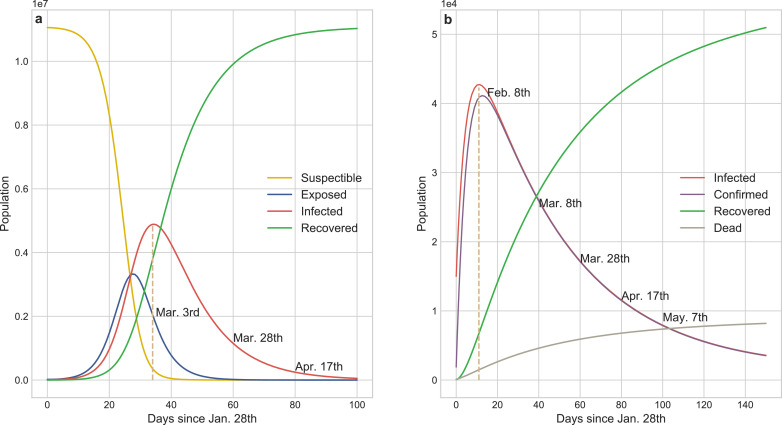
Fig. 6a shows that the SEIR model forecasts the existing infected cases had reached a peak of 4,885,672 on Mar. 3rd which was two orders of magnitude higher than the actual value and the transmission would be effectively controlled before Apr. 17th without external constraints. SEIR inappropriately concludes that more than 50% of the population in Wuhan would be infected in this pandemic, and unfortunately it ignores the death cases caused by COVID-19. Static coefficients based-ICRD (S-ICRD) model predicts the existing infected cases would sub-exponentially increase to 42,729 by Feb. 8th and the pandemic would be basically blocked at May. 27th. It is noticeable that the decline of the infection curve in Fig. 6 b is extraordinarily slower than the clinical statistics resulting from the illogical assumption of constant public health interventions and it explains why the eventual death toll (8,195) markedly higher than the official surveys (3,869) as well.

Fig. 6.

Results from the numerical simulations about COVID-19 transmission tendency of SEIR and S-ICRD models. a SEIR predicts that the existing infected cases would reach a peak of 4,885,672 on Mar. 3rd and the pandemic would be basically blocked on Apr. 17th in Wuhan. More than half of the population would be infected by COVID-19 but the fraction of exposed population is less than the infected population which is inconsistent with the observation. b S-ICRD predicts that the peak of the existing infected cases is 42,729 on Feb. 8th and the epidemic alert would be lifted after May. The forecasted number of infections is consistent with the actual data but the relative crucial time points and the final deaths have a great deviation with the observation in Wuhan since the constant coefficients are inappropriate to simulate the transmission dynamics of COVID-19.

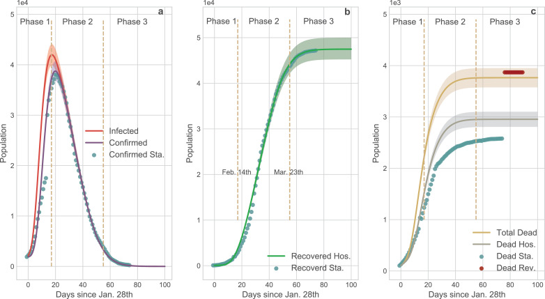
Compared with the SEIR and S-ICRD, the dynamic coefficients based-ICRD model (D-ICRD) has infinitesimal mean square errors (MSE) with the data released by NHC (Fig. 7). D-ICRD estimates that the existing infected and confirmed cases would dramatically raise to their peaks (41986, 38758) on Feb. 14th and 17th respectively (Fig. 7 a), approximately consisting with the practical inflexion: Feb. 18th (38020). In Phase 1, the incomplete identification policies and limited testing techniques contribute to the large gap between the infected and confirmed curves, whereas they gradually coincide with the strengthening of surveillance in phase 2. The truth-values of the recovered cases are always located in the 95% confidence interval (CI) of the curve predicted by D-ICRD but the estimated values are slight higher since the patients who are spontaneously recovered were excluded in the statistics (Fig. 7 b). The death cases calculated by D-ICRD eccentrically deviate from the statistical data before Mar. 8th in Fig. 7 c. Until Apr. 17th, the government announced that there were 1290 missing victims in the initial collecting stage and then increased death cases to 3869 that located in the 95% CI [3576, 3952] of the predicted value.

Fig. 7.

Comparison of the results generated by D-ICRD model and the time series data released by NHC. In this figure the dots denote official data and the curves denote the data calculated by D-ICRD in which the shadow areas denote the 95% confidence interval (CI). The entire pandemic duration in Wuhan is divided into three phases: Phase 1 [Jan. 23th - Feb. 14th]; Phase 2 [Feb.15 - Mar. 23th]; Phase 3 [Mar. 24th - ]. Sta. denotes the official statistical data and Hos. denotes the data counted in hospitals. a the curves of the existing infected and confirmed cases. The gap between the infected curve and the confirmed curve indicates the number of the infected but unconfirmed group [36]. Most dots are located in the shadow areas except for Phase 1 because the health authorities clarified that there were many infected cases of underreporting. b The curve of recovered cases. The calculated data is slightly larger than the amounts counted in hospitals since the spontaneously curative patients are not included and a few medical institutions failed to connect with the information systems in time. c The curve of death cases. Blue dots denote the originally released data and the red dots denote the revised data from NHC. According to the revised data, mortality is seriously underestimated at Phase 1 and Phase 2, and the yellow curve is more representative of the death trend of COVID-19 pandemic. (For interpretation of the references to colour in this figure legend, the reader is referred to the web version of this article.)

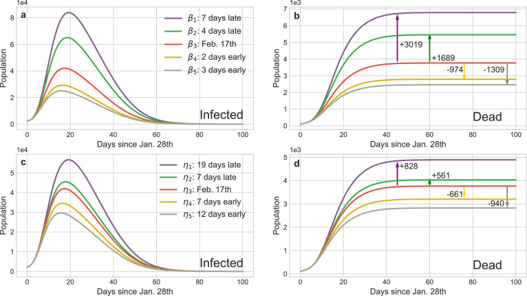
Fig. 5 straightway illustrates that controlling b (or v) can accurately regulate the implement schedule of the isolation (identification) policy and the corresponding results are shown in Fig. 8 . The peaks of the existing infected cases would reduce 12,725 or 17,009 if the isolation policy were executed 2 or 3 days in advance respectively, and thousands of innocent individuals would be saved (Fig. 8 b). Inversely, postponing the quarantine policy for 4 (or 7) days would induce another 15,900 (or 53,753) people to be infected and increase the death toll to 5454 (or 6,783). The advancement or delay of the identification policy would also cause similar results, but their influence is softer than the isolation policy. For instance, the comprehensive identification order issued 7 or 12 days earlier would protect 9567 or 15, 709 people from infection, respectively. Meanwhile, benefiting from the quarantine of suspected persons, medical pressure would be relieved and then 661 or 940 sufferers could be rescued from death. Nevertheless, if such policy was delayed for 17 days, more than a quarter of contacts would be infected or die considering that the increasing of suspected nodes on social networks incredibly shorten their connections with the healthy nodes. Fig. 9 shows reinforcing or weakening the implement intensity of these policies could also result in the suppression or diffusion of the epidemic. Accordingly, the above evidences definitely exhibit that this pandemic is extremely sensitive to the public health interventions, particularly in the initial stage, which can forcefully cut off the possible transmission routes of COVID-19.

Fig. 8.

Impact of the implement time of isolation and identification policies on the transmission tendency of COVID-19 in Wuhan. The red curves are the results of the baseline policies selected in Fig. 5 and the other curves’ colors are matched with Fig. 5 representing advance or delay the corresponding policy. The arrows show the increment or decrement of the death cases compared with the baseline of different policies. a and c The curves of infected cases calculated by the dynamical coefficient α (isolation policy) and η (identification policy) in Fig. 5, respectively. b and d The curves of deaths corresponding to a and c and they provide the statistic evidences how public health interventions save the lives of people. (For interpretation of the references to colour in this figure legend, the reader is referred to the web version of this article.)

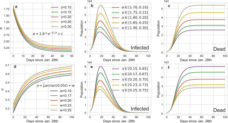
Fig. 9.

Impact of the implement intensity of the isolation and identification policies on the transmission tendency of COVID-19 in Wuhan. a and d illustrate different intervals of α (the isolation intensity) and η (the identification intensity), respectively. b and e The curves of infections corresponding to a and d. c and f The curves of deaths corresponding to a and d.

4.2. Quantify the impact of other dynamical coefficient on the spread of COVID-19

Dynamical daily isolation rateα: The default α in our experiments is :

$$\alpha =1.6*e^{-0.1t}+0.2,\alpha \in [1.8,0.2]$$

In Fig. 8, we have discussed that the implement schedule of the isolation policy can extensively affect the infected cases and death cases in the pandemic. Furthermore, we also can reinforce or weaken the intensity of the relative policy through expanding or reducing the boundaries of α (change parameter c). Fig. 9 provides the statistical evidences about the suppression or diffusion effects of increasing or decreasing the intensity of isolation policy to the spread of COVID-19. If the isolation policy is implement perfunctorily, the peak of the infection curve would dramatically increase (Fig. 9 b) and the accumulation of the death toll would accelerate subsequently (Fig. 9 c). Conversely, if this policy is implemented thoroughly, the aggregate infected cases would distinctly reduce and then the death curve would be remained at a low level during the entire pandemic.

Dynamical daily confirmed isolation rateβin confirmed group: The default β in our experiments is:

$$\beta =\frac{0.2}{\pi }\arctan \left(2t\right)+0.9,\beta \in [0.9,1]$$

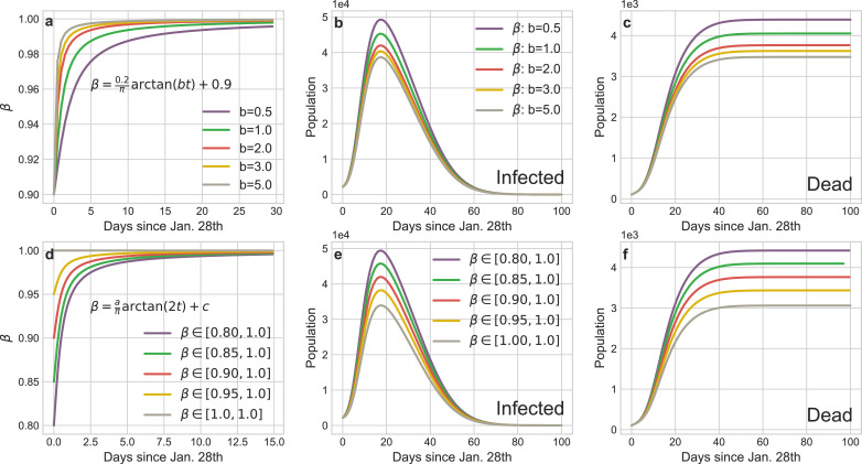
Limited to the lack of medical facilities, many confirmed patients cannot be quarantined and β reflects the fraction of the isolated confirmed patients to the total confirmed patients. According to the transmission mechanism of virus (Fig. 3), this group is of the most dangerous sources of infection on social networks. Fig. 10 shows the severe consequences of untimely isolating such people. In Wuhan, the large-scale construction and rapid delivery of the shelter hospitals eminently contribute to heighten the isolation rate β of infected patients. Correspondingly, relative to the baselines, we speed up the convergence of β (Fig. 10 a) and increase the low bound of β (Fig. 10 d) respectively. Based on the tendency of the infection and death curves, we can safe conclude that the swiftly and comprehensive implement of the isolation policy for infectors has effectively mitigate the spread of COVID-19.

Fig. 10.

Impact of the implement schedule and intensity of the isolation policy for infectors on the transmission tendency of COVID-19 in Wuhan. a The curves of different implement schedule of the isolation policy for infectors (tuning b). d The curves of different implement intensity of the isolation policy for infectors (tuning a and c). b and e The curves of infections corresponding to a and d. c and f The curves of deaths corresponding to a and d.

Dynamical daily investigation rateη: The default η in our experiments is:

$$\eta =\frac{1}{\pi }*\arctan (0.05*t)+0.2,\eta \in [0.2,0.7]$$

Similarly, Fig. 8 shows the impact of the implement schedule of identification policy on the propagation tendency of COVID-19. Fig. 9 illustrates the strength of the corresponding policy can also exacerbate or mitigate the epidemic. In Wuhan, the communities identify the symptomatic or pre-symptomatic infectors through temperature reports and footprint tracking of the entire population. This policy significantly increases the daily identification rate and the simulation results (Fig. 9 e-f) show weakening it would dramatically accelerate the spread of the epidemic. On the contrary, the number of infectors would markedly drop and thousands of people would be saved with the strengthen of this policy.

Dynamical daily cureσ and mortality κ rate: The default σ and κ in our experiments are:

$$\begin{array}{ccc}\hfill \sigma & =& 0.08638*\arctan \left(0.0427\right(t-44.79\left)\right)+0.09663\hfill \\ \hfill \kappa & =& 0.01166*e^{-0.06919t}\hfill \end{array}$$

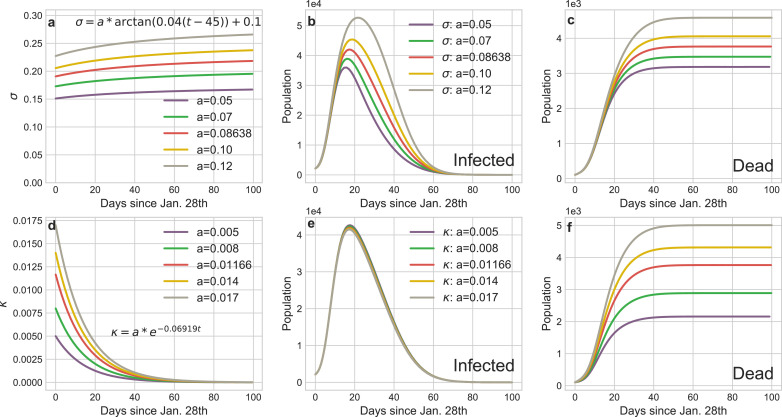
The variation of cure or mortality rates mainly depend on the healthcare capacity of the regional medical systems. Fig. 11 shows the increase of daily cure rate can obviously curb the infection tendency, especially in the mitigation stage (Phase 2). The variation of mortality rate hardly affects the infected curves but it determines the final death toll of the pandemic.

Fig. 11.

Impact of the variations of cure rate or morality on the transmission tendency of COVID-19 in Wuhan. a The curves of dynamic daily cure rate over the entire epidemic period. d The curves of dynamic daily morality rate over the entire epidemic period. b and e The curves of infections corresponding to a and d. c and f The curves of deaths corresponding to a and d.

5. Discussion

Due to the Wuhan government implemented mandatory closures at the early stage of the epidemic to prohibit the free movement of population and issued home quarantine order to isolate internal social contacts during the Spring festival, Wuhan is an ideal research object about the transmission of COVID-19, in which we can detect the general propagation laws about this pandemic. Based on the transmission mechanisms and physicochemical properties of coronavirus, in this paper, we builded a epidemic model named D-ICRD to observe the dynamical change of the existing infected cases, the existing confirmed cases, the cumulative recovered cases and the cumulative deceased cases over time in Wuhan. Besides, our model could also deduce other significant pandemic indexes such that cumulative infected cases, cumulative confirmed cases, new suspected cases etc. Functionally, D-ICRD could not only display the characteristic of nature virus transmission but also precisely quantify the influence of the extra containments on the spread of COVID-19.

We designed the dynamical coefficients associating with the implement schedule and intensity of the relative policies to simulate the transmission environment of COVID-19 in Wuhan. Compared with the static coefficients, the dynamical coefficients can more penetratingly capture the rational adjustment of social responses to the severity of the epidemic. For example, many classical models assume the constant basic reproduction number but we believe that it changes with the intervention factors and eventually this change is mapped on the transmission coefficient α in D-ICRD. Moreover, the improvement of therapy and the use of specific medicines would significantly affect the cure rate and mortality. Based on this, D-ICRD entirely reproduced the time series data released by NHC, and it balances robustness and agility.

Then, we subtly regulated the implement schedule or intensity of these interventional policies through changing the derived functions or boundaries of the corresponding dynamical coefficients to verify the contribution of such policies to suppress the epidemic. The statistical evidences show the forceful public health interventions can effectively suppress or even block the outbreak based on Wuhan’s experiences although COVID-19 has extremely strong infectivity (droplet transmission and suspected aerosol transmission [37]) and lethality (CFR  >  7.69% in Wuhan, before Feb. 20th). We found that the infected and death cases would sharply decrease if the quarantine strategies could be promulgated slightly in advance. Nevertheless, D-ICRD indicates postponing such plans would cause additional millions of infected population worldwide, and undoubtedly the catastrophic consequences of abrogating these ordinances are uncountable. Furthermore, the intensity of the isolation and identification polices would determine the trend of the pandemic as well. We suggest that the governments or communities should adopt the containments such as comprehensive investigating and tracking the temperature and traces information about the residents, immediately isolating the suspected and diagnosed infected individuals to prevent the spread of COVID-19 on social networks. Although such near-compulsory national policies may cause severe economic recession or ethical problems, we must realize that society is a community of life composed of all human beings, and we profoundly influence each other whereupon we should collaborate to fight this vital pandemic together. Given that there are no target therapeutics or vaccine currently, each of us should cooperate with these policies in a responsible manner, isolate ourselves from others, form an island, and ultimately prevent the spread of the virus.

Data availability

The data used in this work is mainly released by NHC (5) and partly collected from Johns Hopkins University, WHO, and CDC. On Apr. 17, 2020, Chinese authorities modified the number of infected cases and death cases because of the omission and false positives in the early transmission stage of COVID-19. Therefore, we believe that the final reported numbers are consistent with the actual values, but there might be a relatively large bias between the daily released data and its corresponding truth values. For this reason, we adopted the 95% confidence interval to assess the consistency between the predicted values and the reference data. All data used in the paper are available at: https://github.com/LuckyYubo/Code-For-ICRD/tree/master/Data.

Code availability

The code used for our analyses is publicly available at: https://github.com/LuckyYubo/Code-For-ICRD.

Declaration of Competing Interest

The authors declare that they have no known competing financial interests or personal relationships that could have appeared to influence the work reported in this paper.

References

- 1.Xu B., Gutierrez B., Mekaru S., Sewalk K., Goodwin L., Loskill A., et al. Epidemiological data from the COVID-19 outbreak, real-time case information. Sci Data. 2020;7(1):1–6. doi: 10.1038/s41597-020-0448-0. [DOI] [PMC free article] [PubMed] [Google Scholar]
- 2.Organization W. H., et al. Coronavirus disease 2019 (COVID-19): situation report, 742020;.
- 3.Wölfel R., Corman V.M., Guggemos W., Seilmaier M., Zange S., Müller M.A., et al. Virological assessment of hospitalized patients with COVID-2019. Nature. 2020:1–10. doi: 10.1038/s41586-020-2196-x. [DOI] [PubMed] [Google Scholar]
- 4.Shi H., Han X., Jiang N., Cao Y., Alwalid O., Gu J., et al. Radiological findings from 81 patients with COVID-19 pneumonia in Wuhan, China: a descriptive study. Lancet Infect Dis. 2020 doi: 10.1016/S1473-3099(20)30086-4. [DOI] [PMC free article] [PubMed] [Google Scholar]
- 5.Bourouiba L. Turbulent gas clouds and respiratory pathogen emissions: potential implications for reducing transmission of COVID-19. JAMA. 2020 doi: 10.1001/jama.2020.4756. [DOI] [PubMed] [Google Scholar]
- 6.Peeri N.C., Shrestha N., Rahman M.S., Zaki R., Tan Z., Bibi S., et al. The SARS, MERS and novel coronavirus (COVID-19) epidemics, the newest and biggest global health threats: what lessons have we learned? Int J Epidemiol. 2020 doi: 10.1093/ije/dyaa033. [DOI] [PMC free article] [PubMed] [Google Scholar]
- 7.Pastorino B., Touret F., Gilles M., de Lamballerie X., Charrel R.N.. Evaluation of heating and chemical protocols for inactivating SARS-CoV-2. bioRxiv2020;. [DOI] [PMC free article] [PubMed]
- 8.Sajadi M.M., Habibzadeh P., Vintzileos A., Shokouhi S., Miralles-Wilhelm F., Amoroso A.. Temperature and latitude analysis to predict potential spread and seasonality for COVID-19. Available at SSRN 35503082020;. [DOI] [PMC free article] [PubMed]
- 9.Luo C., Yao L., Zhang L., Yao M., Chen X., Wang Q., et al. Possible transmission of severe acute respiratory syndrome coronavirus 2 (SARS-CoV-2) in a public bath center in Huaian, Jiangsu province, China. JAMA Netw Open. 2020;3(3):e204583. doi: 10.1001/jamanetworkopen.2020.4583. [DOI] [PubMed] [Google Scholar]
- 10.Huang C., Wang Y., Li X., Ren L., Zhao J., Hu Y., et al. Clinical features of patients infected with 2019 novel coronavirus in Wuhan, China. Lancet. 2020;395(10223):497–506. doi: 10.1016/S0140-6736(20)30183-5. [DOI] [PMC free article] [PubMed] [Google Scholar]
- 11.Lauer S.A., Grantz K.H., Bi Q., Jones F.K., Zheng Q., Meredith H.R., et al. The incubation period of coronavirus disease 2019 (COVID-19) from publicly reported confirmed cases: estimation and application. Ann Intern Med. 2020 doi: 10.7326/M20-0504. [DOI] [PMC free article] [PubMed] [Google Scholar]
- 12.Lurie N., Saville M., Hatchett R., Halton J. Developing COVID-19 vaccines at pandemic speed. N Engl J Med. 2020 doi: 10.1056/NEJMp2005630. [DOI] [PubMed] [Google Scholar]
- 13.Hartley D.M., Perencevich E.N. Public health interventions for COVID-19: emerging evidence and implications for an evolving public health crisis. JAMA. 2020 doi: 10.1001/jama.2020.5910. [DOI] [PubMed] [Google Scholar]
- 14.Hellewell J., Abbott S., Gimma A., Bosse N.I., Jarvis C.I., Russell T.W., et al. Feasibility of controlling COVID-19 outbreaks by isolation of cases and contacts. Lancet Global Health. 2020 doi: 10.1016/S2214-109X(20)30074-7. [DOI] [PMC free article] [PubMed] [Google Scholar]
- 15.Kraemer M.U., Yang C.-H., Gutierrez B., Wu C.-H., Klein B., Pigott D.M., et al. The effect of human mobility and control measures on the COVID-19 epidemic in china. Science. 2020 doi: 10.1126/science.abb4218. [DOI] [PMC free article] [PubMed] [Google Scholar]
- 16.Pan A., Liu L., Wang C., Guo H., Hao X., Wang Q., et al. Association of public health interventions with the epidemiology of the COVID-19 outbreak in Wuhan, China. JAMA. 2020 doi: 10.1001/jama.2020.6130. [DOI] [PMC free article] [PubMed] [Google Scholar]
- 17.Tian H., Liu Y., Li Y., Wu C.-H., Chen B., Kraemer M.U., et al. An investigation of transmission control measures during the first 50 days of the COVID-19 epidemic in China. Science. 2020 doi: 10.1126/science.abb6105. [DOI] [PMC free article] [PubMed] [Google Scholar]
- 18.Prem K., Liu Y., Russell T.W., Kucharski A.J., Eggo R.M., Davies N., et al. The effect of control strategies to reduce social mixing on outcomes of the COVID-19 epidemic in Wuhan, China: a modelling study. Lancet Public Health. 2020 doi: 10.1016/S2468-2667(20)30073-6. [DOI] [PMC free article] [PubMed] [Google Scholar]
- 19.Li Q., Guan X., Wu P., Wang X., Zhou L., Tong Y., et al. Early transmission dynamics in Wuhan, China, of novel coronavirus–infected pneumonia. N Engl J Med. 2020 doi: 10.1056/NEJMoa2001316. [DOI] [PMC free article] [PubMed] [Google Scholar]
- 20.Wu J.T., Leung K., Bushman M., Kishore N., Niehus R., de Salazar P.M., et al. Estimating clinical severity of COVID-19 from the transmission dynamics in Wuhan, China. Nat Med. 2020:1–5. doi: 10.1038/s41591-020-0822-7. [DOI] [PMC free article] [PubMed] [Google Scholar]
- 21.Leung N.H., Chu D.K., Shiu E.Y., Chan K.-H., McDevitt J.J., Hau B.J., et al. Respiratory virus shedding in exhaled breath and efficacy of face masks. Nat Med. 2020:1–5. doi: 10.1038/s41591-020-0843-2. [DOI] [PMC free article] [PubMed] [Google Scholar]
- 22.Ferretti L., Wymant C., Kendall M., Zhao L., Nurtay A., Abeler-Dörner L., et al. Quantifying SARS-CoV-2 transmission suggests epidemic control with digital contact tracing. Science. 2020 doi: 10.1126/science.abb6936. [DOI] [PMC free article] [PubMed] [Google Scholar]
- 23.Maier B.F., Brockmann D. Effective containment explains subexponential growth in recent confirmed COVID-19 cases in China. Science. 2020 doi: 10.1126/science.abb4557. [DOI] [PMC free article] [PubMed] [Google Scholar]
- 24.Kissler S.M., Tedijanto C., Goldstein E., Grad Y.H., Lipsitch M. Projecting the transmission dynamics of SARS-CoV-2through the postpandemic period. Science. 2020 doi: 10.1126/science.abb5793. [DOI] [PMC free article] [PubMed] [Google Scholar]
- 25.Wurtzer S., Marechal V., Mouchel J.-M., Moulin L.. Time course quantitative detection of SARS-CoV-2 in parisian wastewaters correlates with COVID-19 confirmed cases. medRxiv2020;.
- 26.Gudbjartsson D.F., Helgason A., Jonsson H., Magnusson O.T., Melsted P., Norddahl G.L., et al. Spread of SARS-CoV-2 in the icelandic population. N Engl J Med. 2020 doi: 10.1056/NEJMoa2006100. [DOI] [PMC free article] [PubMed] [Google Scholar]
- 27.Fanelli D., Piazza F. Analysis and forecast of COVID-19 spreading in china, italy and france. Chaos Solitons Fractals. 2020;134:109761. doi: 10.1016/j.chaos.2020.109761. [DOI] [PMC free article] [PubMed] [Google Scholar]
- 28.Tsang T.K., Wu P., Lin Y.L.Y., Lau E., Leung G.M., Cowling B.J.. Impact of changing case definitions for COVID-19 on the epidemic curve and transmission parameters in mainland china. medRxiv2020;. [DOI] [PMC free article] [PubMed]
- 29.Salathé M., Althaus C.L., Neher R., Stringhini S., Hodcroft E., Fellay J., et al. COVID-19 epidemic in switzerland: on the importance of testing, contact tracing and isolation. Swiss Med Wkly. 2020;150(1112) doi: 10.4414/smw.2020.20225. [DOI] [PubMed] [Google Scholar]
- 30.Hethcote H.W. The mathematics of infectious diseases. SIAM Rev. 2000;42(4):599–653. [Google Scholar]
- 31.Bao L., Deng W., Gao H., Xiao C., Liu J., Xue J., et al. Reinfection could not occur in SARS-CoV-2 infected rhesus macaques. BioRxiv. 2020 [Google Scholar]
- 32.Kucharski A.J., Russell T.W., Diamond C., Liu Y., Edmunds J., Funk S., et al. Early dynamics of transmission and control of COVID-19: a mathematical modelling study. Lancet Infect Dis. 2020 doi: 10.1016/S1473-3099(20)30144-4. [DOI] [PMC free article] [PubMed] [Google Scholar]
- 33.Li R., Pei S., Chen B., Song Y., Zhang T., Yang W., et al. Substantial undocumented infection facilitates the rapid dissemination of novel coronavirus (SARS-CoV2) Science. 2020 doi: 10.1126/science.abb3221. [DOI] [PMC free article] [PubMed] [Google Scholar]
- 34.Chinazzi M., Davis J.T., Ajelli M., Gioannini C., Litvinova M., Merler S., et al. The effect of travel restrictions on the spread of the 2019 novel coronavirus (COVID-19) outbreak. Science. 2020 doi: 10.1126/science.aba9757. [DOI] [PMC free article] [PubMed] [Google Scholar]
- 35.Huang Y., Dong H., Zhang W., Lu J. Stability analysis of nonlinear oscillator networks based on the mechanism of cascading failures. Chaos Solitons Fractals. 2019;128:5–15. [Google Scholar]
- 36.Mallapaty S. Antibody tests suggest that coronavirus infections vastly exceed official counts. Nature. 2020 doi: 10.1038/d41586-020-01095-0. [DOI] [PubMed] [Google Scholar]
- 37.Liu Y., Ning Z., Chen Y., Guo M., Liu Y., et al. Aerodynamic analysis of SARS-CoV-2 in two Wuhan hospitals. Nature. 2020 doi: 10.1038/s41586-020-2271-3. [DOI] [PubMed] [Google Scholar]
Associated Data
This section collects any data citations, data availability statements, or supplementary materials included in this article.
Data Availability Statement