Direct Adjusted Survival and Cumulative Incidence Curves for Observational Studies

Editors Note

Large randomized clinical trials testing the impact of subject-, disease- and transplant-related co-variates on outcomes amongst recipients of haematopoietic cell transplants are uncommon. For example, who is the best donor, which is the best pretransplant conditioning regimen or the best regimen to prevent or treat acute and/or chronic graft-versus-host disease. To answer these questions we often rely on analyses of data from large observational datasets such as those of the Center for International Blood and Marrow Transplant Research (CIBMTR) and the European Society for Blood and Marrow Transplantation (EBMT). Such analyses have proved extremely important in advancing the field. However, in contrast to randomized trials, we cannot be certain potentially important prognostic or predictive co-variates are balanced between cohorts selected for comparison from an observational dataset, a limitation which can lead to incorrect conclusions. In the typescript which follows the authours describe a method to adjust for known imbalances in co-variates and get a closer approximation of the truth. They give two examples, the impact of a new pretransplant conditioning regimen on disease-free survival (DFS) in subjects with Ewing sarcoma and the impact of donor type on treatment-related mortality (TRM) and leukaemia relapse in subjects with acute leukaemia.

Direct adjusted survival and cumulative incidence function (CIF) analyses are an important step forward. These analyses can be done using available statistical packages and we encourage readers to use them rather than reporting unadjusted analyses. Finally, we must emphasize direct adjustment can only be done for know prognostic or predictive co-variates, not unknown co-variates. Unknown co-variates will be balanced in randomized trials which is why we do them. So direct adjustment is an important step forward but not a perfect substitute for randomized trials. But any step forward is important. To quote Laozi: 千里之行始於足下 (A journey of a thousand miles begins with a single step).

Introduction

When we want to compare safety or efficacy of two therapies it is common to use well-known statistical techniques. For randomized clinical trials this is frequently done by comparing using crude Kaplan-Meier survival curves [1]. When there are competing risks for outcome such as for leukaemia recurrence and graft-versus-host disease (GvHD) the comparison often uses unadjusted cumulative incidence function (CIF) curves [2]. In contrast, for observational studies regression models such as a Cox model or other more flexible models are commonly used [3, 4]. Frequently, treatment effect is calculated based on regression models and reported as unadjusted survival or CIF curves. However, these unadjusted comparisons can be biased and do not account for potential difference in prognostic variables between cohorts. Not surprisingly, results of these unadjusted comparisons of treatment effects often differ from treatment effects estimated from regression models in which confounding co-variate distributions are adjusted for. Here, we explain the use of regression model-based direct adjusted survival and CIF curves which account for competing risk data [5–8]. These direct adjusted probabilities estimate likelihoods of outcomes in populations with similar prognostic or predictive co-variates. These adjustments are important when we try to imply causal inference which we discussed in a prior typescript in this series [9, 10].

Crude survival and CIF estimates and confounding effects

When outcomes of time-to-event data such as survival after a transplant are right censored without adjusting for competing risks the Kaplan-Meier estimator is commonly used to present this probability. Hypothesis testing of potential differences between cohorts is often tested using the log-rank test [11]. In contrast, when the outcome has competing risks, such as leukaemia relapse where treatment-related mortality (TRM, i.e. death without relapse) preludes its occurrence, CIF is used to estimate incidence rates of the event in the cohorts and hypothesis-testing often uses the Gray test [12].

The Kaplan-Meier estimator and CIFs are widely supported by statistical packages such as SAS and R. Many published studies present univariate unadjusted plots of the outcomes we discuss. However, unlike the Cox proportional hazards model or the Fine-Gray model where confounding effects of other co-variates can be statistically adjusted for, there is no adjustment for potentially confounding variables [3, 13]. Using unadjusted curves is usually not a substantial problem when data are derived from randomized trials or matched-pair analyses because potential confounders eliminated by randomization or matching. However, data from observational studies are often imbalanced with different distributions of co-variates between cohorts. When imbalanced co-variates are associated with the outcome of interest they introduce a confounding bias on the treatment effect when there is no adjustment in the analysis [14]. Here, crude estimates from the Kaplan-Meier estimator or CIF often disagree with the adjusted hazard ratio (HR) or sub-distribution HR estimates from the Cox proportional hazard model or the Fine-Gray model and cause contradictory interpretations of the results. For example, if there were more subjects with advanced leukaemia in one cohort compared with a comparison cohort an unadjusted analysis might suggest a difference between two pretransplant conditioning regimens whereas an adjusted analysis might suggest no difference. Is there a way to reconcile these different conclusions?

Example of Imbalanced Data Causing Biased Survival and CIF Estimates

In a data set of 76 subjects with Ewing sarcoma [15], lactic acid dehydrogenase (LDH) level, a prognostic variable for disease-free survival (DFS), is imbalanced between the conventional and experimental therapy cohorts. Assume 66 percent of subjects in the conventional therapy cohort have a high LDH level compared with only 25 percent in the experimental therapy cohort (Chi-square P-value, 0.0006). In the unadjusted DFS comparison the log-rank test P-value is 0.032 indicating the Kaplan-Meier curves of DFS between the cohort are significantly different (Figure 1A). A Cox regression model analysis without adjusting for LDH level has a Hazard Ratio (HR) of 0.53 (95% confidence interval (CI): 0.30, 0.96) with a P-value 0.035, again indicating statistical significance. However, after adjusting for LDH level the Cox proportional hazards model has a HR of 1.12 (95% CI: 0.59, 2.11) with a P-value 0.734 suggesting the experimental therapy is no better than the conventional therapy. The Cox model also shows the HR for high LDH level is 7.99 (95% CI: 3.96–16.13) with a P-value <0.0001. These data indicate the seeming benefit of the experimental therapy is wrong and that the difference in DFS is the result of the imbalance in LDH levels between the cohorts.

Figure 1. Comparison of survival curves for DFS with or without adjustment for LDH level in subjects with Ewing sarcoma.

Panel A: Unadjusted Kaplan-Meier survival curves for DFS;

Panel B: Direct adjusted survival curves for DFS;

Panel C: Differences in direct adjusted survival curves for DFS (shaded area: 95% confidence band)

As another example of the problem of unadjusted analyses we consider an observational dataset of 623 subjects from the CIBMTR registry which compared TRM, leukaemia relapse and leukaemia-free survival (LFS) between recipients of transplants from HLA-identical siblings versus from HLA-matched unrelated donors for early- or intermediate-stage acute leukemia [16]. There was a significant difference between the cohorts in proportions of early- versus intermediate-stage leukaemia state. In the HLA-identical sibling cohort 75 percent of subjects had early leukaemia versus 29 percent in the HLA-matched unrelated donor cohort (Chi-square P-value <0.0001). The unadjusted CIF curves for TRM and relapse by donor type are displayed in Figures 2-A and -C. Without adjustment for leukaemia state the sub-distribution HRs from the Fine-Gray model is 2.43 (1.65, 3.58) for TRM with a P-value <0.0001 and 0.50 (0.24, 1.04) for relapse with a P-value 0.063. After adjustment the sub-distribution HR for TRM becomes 1.83 (1.18, 2.84) with a P-value of 0.007 and the sub-distribution HR for relapse becomes 0.40 (0.19, 0.84) with a P-value 0.016. Although the P-values for TRM from both models are statistically significant the confounding effect of leukaemia state exaggerates the HR estimates of the association between donor type and TRM in the unadjusted model (2.43 versus 1.83). The P-value for relapse indicates that the likelihood the null hypothesis there is no difference becomes very much more unlikely in the adjusted analysis. This confounding effect also operates in analyses of LFS. As displayed in Figure 3-A the log-rank test P-value for the unadjusted Kaplan-Meier curves for LFS is 0.012 indicating a significant association between donor type and LFS. The HR for LFS from an unadjusted Cox regression is 1.54 (1.10,2.17) with a P-value 0.013. After adjustment however the HR is 1.09 (0.76, 1.57) with a P-value 0.632 showing no association between donor type and LFS. The seeming association from the unadjusted model is caused by the imbalance in distribution of leukaemia states and its strong association with LFS (HR: 2.06 [1.59, 2.67; P-value < 0.0001).

Figure 2. Comparison of CIF curves for TRM and relapse with or without adjustment for leukaemia state.

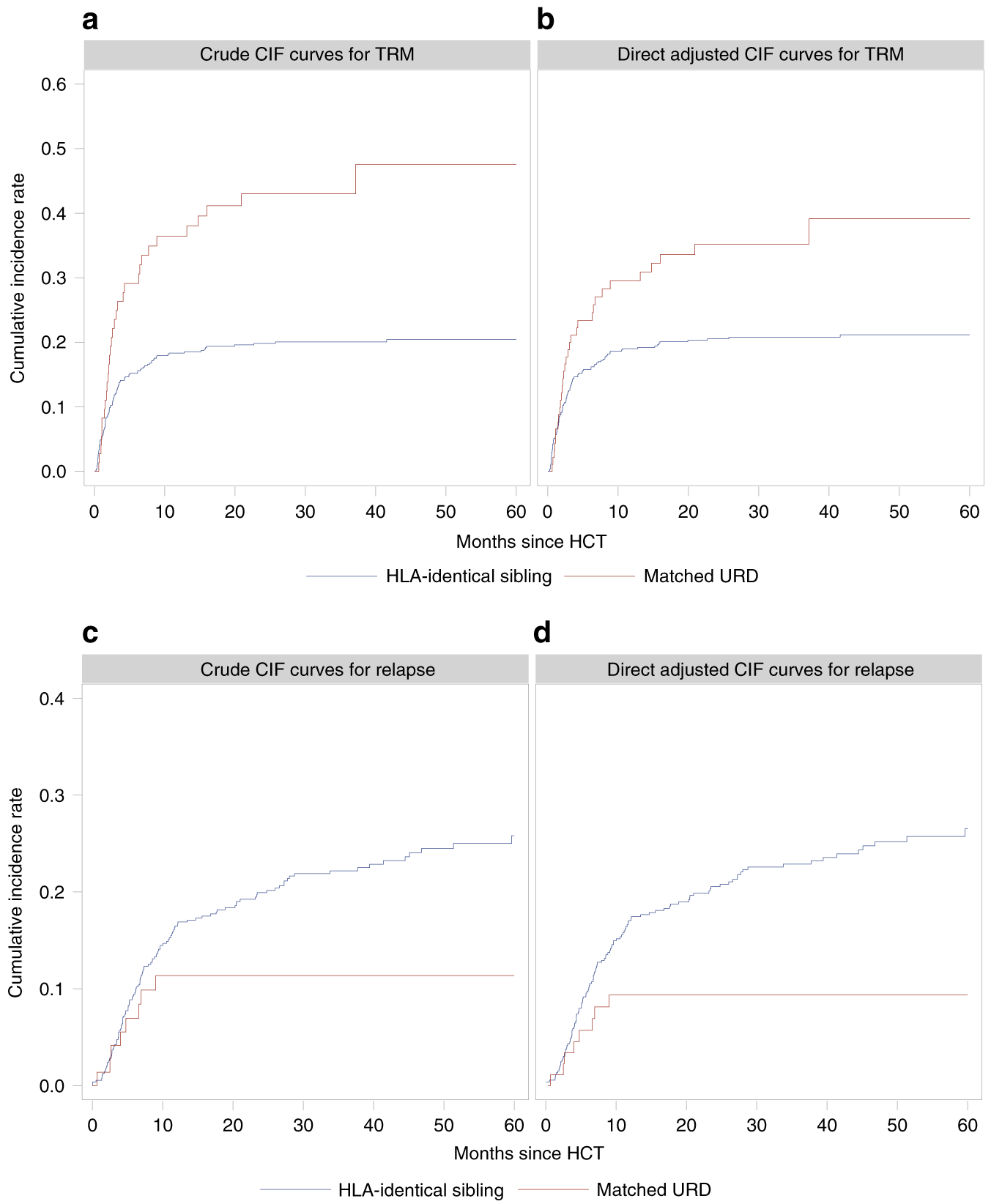
Panel A: Unadjusted CIF curves for TRM;

Panel B: Direct adjusted CIF curves for TRM;

Panel C: Unadjusted CIF curves for relapse;

Panel D: direct adjusted CIF curves for relapse

Figure 3. Comparison of survival curves for LFS with or without adjustment for leukaemia state.

Panel A: Unadjusted Kaplan-Meier survival curves for LFS;

Panel B: Direct adjusted survival curves for LFS;

Panel C: Differences in direct adjusted survival curves for DFS (shaded area: 95% confidence band)

Direct Adjusted Survival and Cumulative Incidence Functions

Survival functions can be directly derived from cumulative hazard functions using the Cox proportional hazards model and its estimator for the cumulative hazard functions [17], Consequently, it is possible to generate multi-variate adjusted survival curves based on the average values of the covariates [18]. However, this method can be difficult to interpret as the average of a categorical co-variate may not be scientifically meaningful [18]. More importantly, this approach does not account for the sample variability of different subjects between the treatment cohorts and can be mis-leading regarding the true treatment effect [18].

An alternative approach called direct adjusted survival curves relies on averaging the Cox model-derived survival curve of each subject from the entire pooled sample [5, 6, 7]. Because this method averages over the pooled sample results are more representative of the underlying data and can be interpreted as the estimated probabilities for each treatment in a population with similar prognostic variables. Using a Cox model stratified by treatment cohort also allows treatment effect to vary over time [7]. The confidence limits and point-wise P-values can be derived from the standard errors of the difference between two direct adjusted survival curves for comparisons and hypothesis-testing at any timepoint [19]. For simultaneous comparison between two direct adjusted survival curves, confidence bands can be constructed by simulation for visualized comparisons [20]. Simultaneous P-value can also be derived to test the hypothesis of no treatment effect (null hypothesis) over a time interval [21]. Similarly, the Fine-Gray model provides a direct link between the CIF and the pseudo hazard function (sub-distribution hazard function) [13]. Therefore, for outcomes with competing risks, direct adjusted CIF curves can be derived from averaging CIFs of subjects from the entire pooled sample based on a stratified Fine-Gray model [8]. Likewise, results of this approach represent the estimate cumulative incidences of each treatment in population with similar prognostic variables.

Using this method we can re-examine the Ewing sarcoma data after accounting for the confounding effect of LDH level. Now as shown in Figure 1-B the direct adjusted survival curves for DFS between the cohorts are not significantly different (simultaneous P-value, 0.294) with 1-year and 2-year direct adjusted survival of 69 and 61 percent for the conventional therapy cohort and 77 and 53 percent for the experimental therapy cohort, indicating no statistically significant point-wise differences (point-wise P-values, 0.349 and 0.334 respectively). As shown in Figure 1-C, the 95% confidence band of the difference between the two direct adjusted survival curves also covers the entire zero line across the follow-up period. These results are consistent with the findings from the multi-variate Cox proportional hazards model.

We can also use this method on the CIBMTR dataset. The direct adjusted CIF curves for TRM and relapse after adjusting for leukaemia state are presented in Figure 2-B and -D. 5-year direct adjusted CIF rates for TRM are 21 percent for the HLA-identical sibling donor cohort and 39 percent for the HLA-matched unrelated donor cohort - an 18 percent difference favouring the HLA-identical sibling cohort (point-wise P-value, 0.012). In contrast 5-year crude CIF rates are 20 and 48 percent, a 27 percent difference (point-wise P-value, < 0.001) resulting in a 10 percent increase in difference compared to direct adjusted model. For relapse, the 5-year direct adjusted CIF rates are 27 percent for the HLA-identical sibling donor cohort and 9 percent for the HLA-matched unrelated donor cohort, an 18 percent difference in the opposite direction of TRM (point-wise P-value, < 0.001), compared with 26 and 11 percent for the 5-year crude CIF rates (point-wise P-value, 0.001). As displayed in Figure 3-B and 3-C there is no difference between the direct adjusted survival curves for LFS (simultaneous p-value, 0.235). The 5-year direct adjusted survival rates for LFS are 52 percent for both donor types (point-wise P-value, 0.993). These data all indicate that the direct adjusted CIF curves and survival curves are more representative of the results of the multi-variate Fine-Gray model and Cox proportional hazard model.

Several statistical packages including SAS PHREG are available and can generate the direct adjusted survival curves and CIF curves [7, 8, 21].

Conclusion

In this brief review we show conclusions from analyses of observational datasets are influenced by unbalanced data and can be biased by confounding effects if the unbalanced co-variates are not adjusted for. For right censored time-to-event data the direct adjusted survival curves and the direct adjusted CIF curves are two approaches which can accurately represent the adjusted survival and CIF estimates of the study population with similar prognostic variables. Confidence bands and simultaneous P-values can also be generated for hypothesis testing and evaluating the differences of two direct adjusted survival or CIF curves over a time period.

References

- 1.Kaplan EL and Meier P, Nonparametric estimation from incomplete observations. J Am Stat Assoc, 1958. 53(282): p. 457–481. [Google Scholar]
- 2.Kalbfleisch JD and Prentice RL, The statistical analysis of failure time data. Can J Stat, 1982. 10(1): p. 64–66. [Google Scholar]
- 3.Cox DR, Regression models and life-tables. J R Stat Soc Series B Stat Methodol, 1972. 34(2): p. 187–220. [Google Scholar]
- 4.Scheike TH and Zhang MJ, Flexible competing risks regression modeling and goodness-of-fit. Lifetime Data Analysis, 2008. 14: p. 464–483. [DOI] [PMC free article] [PubMed] [Google Scholar]
- 5.Makuch RW, Adjusted survival curve estimation using covariates. J Chronic Dis, 1982. 35(6): p. 437–43. [DOI] [PubMed] [Google Scholar]
- 6.Chang IM, Gelman R and Pagano M, Corrected group prognostic curves and summary statistics. J Chronic Dis, 1982. 35(8): p. 669–74. [DOI] [PubMed] [Google Scholar]
- 7.Zhang X, Loberiza FR, Klein JP and Zhang MJ, A SAS macro for estimation of direct adjusted survival curves based on a stratified Cox regression model. Computer Methods and Programs in Biomedicine, 2007. 88(2): p. 95–101. [DOI] [PubMed] [Google Scholar]
- 8.Zhang X and Zhang MJ, SAS macros for estimation of direct adjusted cumulative incidence curves under proportional subdistribution hazards models. Computer Methods and Programs in Biomedicine, 2011. 101(1): p. 87–93. [DOI] [PMC free article] [PubMed] [Google Scholar]
- 9.Chen P and Tsiatis AA, Causal inference on the difference of the restricted mean life between two groups. Biometrics, 2001. 57: p. 1030–1038. [DOI] [PubMed] [Google Scholar]
- 10.Zheng C, Dai R, Gale RP and Zhang M -J, Causal inference in randomized clinical trials. Bone Marrow Transplantation, 2019. [DOI] [PubMed] [Google Scholar]
- 11.Andersen PK, Borgan O, Gill R and Keiding N, Linear nonparametric tests for comparison of counting processes, with applications to censored survival data, correspondent paper. International Statistical Review, 1982. 50(3): p. 219–244. [Google Scholar]
- 12.Gray RJ, A class of K-sample tests for comparing the cumulative incidence of a competing risk. Annals of Statistics, 1988. 16(3): p. 1141–1154. [Google Scholar]
- 13.Fine JP and Gray RJ, A proportional hazards model for the subdistribution of a competing risk. Journal of the American Statistical Association, 1999. 94(446): p. 496–509. [Google Scholar]
- 14.Elwood JM, Causal relationships in medicine: a practical system for critical appraisal. Oxford Medical Publications. 1988, Oxford; New York: Oxford University Press; xi, 332 p. [Google Scholar]
- 15.Brereton HD, Simon R, and Pomeroy TC, Pretreatment serum lactate dehydrogenase predicting metastatic spread in Ewing’s sarcoma. Annals of Internal Medicine, 1975. 83(3): p. 352–354. [DOI] [PubMed] [Google Scholar]
- 16.Szydlo R, Goldman JM, Klein JP, Gale RP, Ash RC, Bach FH, et al. , Results of allogeneic bone marrow transplants for leukemia using donors other than HLA-identical siblings. Journal of Clinical Oncology, 1997. 15(5): p. 1767–1777. [DOI] [PubMed] [Google Scholar]
- 17.Breslow N, Contribution to the discussion of paper by D.R. Cox. J R Stat Soc Series B Stat Methodol, 1972. 34(2): p. 216–217. [Google Scholar]
- 18.Nieto FJ and Coresh J, Adjusting survival curves for confounders: a review and a new method. Am J Epidemiol, 1996. 143(10): p. 1059–68. [DOI] [PubMed] [Google Scholar]
- 19.Gail MH and Byar DP, Variance calculations for direct adjusted survival curves, with applications to testing for no treatment effect. Biom J, 1986. 28(5): p. 587–599. [Google Scholar]
- 20.Zhang MJ and Klein JP, Confidence bands for the difference of two survival curves under proportional hazards model. Lifetime Data Analysis, 2001. 7(3): p. 243–54. [DOI] [PubMed] [Google Scholar]
- 21.Wang H and Zhang X, Confidence band for the differences between two direct adjusted survival curves. Journal of Statistical Software, 2016. 70(Code Snippet 2): p. 17 [Google Scholar]