Biomarker Localization from Deep Learning Regression Networks

Abstract

Biomarker estimation methods from medical images have traditionally followed a segment-and-measure strategy. Deep-learning regression networks have changed such a paradigm, enabling the direct estimation of biomarkers in databases where segmentation masks are not present. While such methods achieve high performance, they operate as a black-box. In this work, we present a novel deep learning network structure that, when trained with only the value of the biomarker, can perform biomarker regression and the generation of an accurate localization mask simultaneously, thus enabling a qualitative assessment of the image locus that relates to the quantitative result. We showcase the proposed method with three different network structures and compare their performance against direct regression networks in four different problems: pectoralis muscle area (PMA), subcutaneous fat area (SFA), liver mass area in single slice computed tomography (CT), and Agatston score estimated from non-contrast thoracic CT images (CAC). Our results show that the proposed method improves the performance with respect to direct biomarker regression methods (correlation coefficient of 0.978, 0.998, and 0.950 for the proposed method in comparison to 0.971, 0.982, and 0.936 for the reference regression methods on PMA, SFA and CAC respectively) while achieving good localization (DICE coefficients of 0.875, 0.914 for PMA and SFA respectively, p < 0.05 for all pairs). We observe the same improvement in regression results comparing the proposed method with those obtained by quantify the outputs using an U-Net segmentation network (0.989 and 0.951 respectively). We, therefore, conclude that it is possible to obtain simultaneously good biomarker regression and localization when training biomarker regression networks using only the biomarker value.

I. Introduction

IN medical environments, a biomarker refers to a trait that describes the biological state of a patient. In this definition of [1], image-based biomarkers are inferred from the quantification of any tissue or organ that can be related to a disease. Many biomarkers relate to the area or volume of structures and, to obtain them, a segmentation is performed to delimit the target area or volume before measuring the final value, such paradigm is often referred as “segment-and-measure”. Manual biomarker estimation is often time-consuming, restricting the number of biomarkers readily available in clinical practice. Since the inception of medical image processing, structure segmentation has been one of the main tasks, mainly to facilitate biomarker discovery or their implementation in clinical practice.

Standard “segment-and-measure” methods used mathematical properties of the structures to locate and segment them. In recent years, through the use of machine learning methods, and more particularly, convolutional neural networks, the focus has been on developing a database with images and corresponding segmentations and train a machine learning based method. Obtaining a large enough training database is often expensive, especially when the number of samples required for it to work is large.

Datasets obtained from clinical practice often have the value of the biomarker associated with the image, but no segmentation mask associated with it is stored. To use these datasets, direct biomarker regression methods have emerged. Examples have appeared in [2] or [3], using a deep learning regression framework. While achieving high performance and not requiring intermediate segmentations, these approaches operate as a black-box, not indicating where the measurement is coming from the area of interest, if at all.

In this work, we propose a network structure that regresses the biomarker value while simultaneously producing the location of the structure that has produced such value at a pixel-level resolution. The core of the proposed network is an encoder-decoder segmentation structure that outputs a binary image. Since no reference mask is available, we aggregate the information of the values of such a mask to estimate the biomarker value, which is then compared to the reference standard to train the network. A multiplication step with pixel-based region candidates is performed to reduce the space of possible solutions. The networks are optimized using the ${\mathcal{L}}_2$ cost function between the computed biomarker and the reference standard. An example of the proposed operational block can be found in Fig. 1.

Fig. 1.

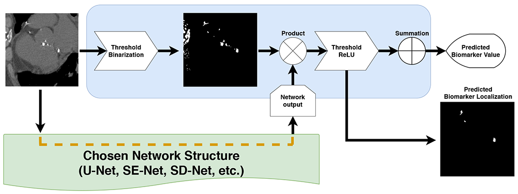
Proposed method block. This structure can be attached to any network to generate both, regression biomarker value and his associated localization.

Inferring attention maps from convolutional neural networks in medical applications is an active area of research. For instance, [4] uses a CNN for pixel-wise lesion detection, the work of [5] describes a system composed of two CNNs, the first one performs a held of view alignment followed by a second network than compute the direct regression of the calcium score, or [6] propose a weakly supervised chest x-net for thoracic diseases classification and lesion localization. Finally, in the context of natural image processing, [7] uses fully CNN for semantic segmentation. However, all these approaches often return low-resolution results, require of prior knowledge not guided by biomarker estimation or the localization maps must be obtained in post-process after modifying the network structure, aspects from which the proposed method does not suffer.

We are going to evaluate the proposed method within the context of three image-based biomarkers: subcutaneous fat area and pectoralis muscle area from 2D axial slices of non-contrast CT images and Agatston score computation in 3D thoracic non-contrast computed tomography images. We further evaluate the proposed method with the regression of liver tumor area from CT axial slices.

Cachexia has been shown to be of clinical relevance in Chronic Obstructive Pulmonary Disease (COPD) and lung cancer as is illustrated by [8] and [9]. Pectoralis muscle and subcutaneous fat areas, measured in computed tomography scans using an axial slice at the level of the transversal aorta, are two biomarkers that have been proven superior to body mass index (BMI) [9]. Such biomarkers have been attempted to automate through the use of atlas-based techniques, as for example in the work of [10], or the standard U-Net network used by [11].

The Coronary Artery Calcification (CAC) is a heart disease that consist in the obstruction by calcium particles in the inside of the coronary arteries. [12] proposed a method to obtain a biomarker value as an indicator of severity. Such biomarker consists in measuring the volume of the calcifications and weighting it by a factor related to the maximum intensity of each individual CAC with an intensity value greater than 130 Hounsheld Units (HU), adding the per lesion value to get a global biomarker value. Recent studies have shown excellent correlation between the Agatston score computed in cardiac ECG-gated CT and in no ECG-gated chest CT[13] Computing the Agatston score is an active area of research. We can find examples of this in the works of [14] who uses a random forest tree for classify a list of coronary artery calcification (CAC) candidates described with a set of features, [15] with a K-Nearest-Neighbor (KNN) classifier or [16] who evaluated some different classification methods including KNN, linear/quadratic discriminant and Support Vector Machine (SVM). In contrast, the work of [17] focus their method in the heart localization prior to the CAC segmentation/measure. More recent work have used convolutional neural networks, for instance [18] used a pair of convolutional networks for, in first place, identifying the candidates voxels and, then, a pixel wise classification as CAC or Non-CAC is performed for obtain the segmentation region and be able to infer the biomarker value from it.

The Liver cancer was the seventh most common type of cancer in 2018, and together with the stomach cancer, represent the second highest number of cancer deaths (both with 8.2% of total cases, around 782,000 each, worldwide) [19]. Tumor localization and quantification are an important task for enabling treatments like radiotherapy [20] or thermal ablations [21], among others. The tumor volume has proven its superiority over the diameter as staging biomarker [22], this raises its importance in automatic systems and makes it possible to use it to identify complex structures from its value.

II. Material and Methods

A. Datasets

COPDGene is a multi-center observational study designed to understand the evolution and genetic determinants of COPD in smokers [23]. 10,000 subjects, with a distribution of non-Hispanic White and African American of 2/3 and 1/3 respectively with ages between 45 and 80 years, have been enrolled in the study and undergone pulmonary non-ECG gated CT scanning with a scanner of at least 16 detectors (GE LS16, VCT-64 and HD750, Philips 16, 40 and 64 Slice, and Philips ICT-128 and ICT-256). For each patient, a CT with full inspiration and normal expiration states was acquired. The inspiratory scans of this database were annotated by independent groups for CAC, PMA and SFA. We therefore consider only those scans for processing.

1. Coronary Artery Calcifications: The Agatston score was computed in 6983 of COPDGene database, forming the dataset in which we train and evaluate the proposed method. We automatically select a region of interest (ROI) centered around the heart in each CT scan using the method of [24] and [25]. We use a prefixed ROI size of 192 × 192 × 224 to avoid the need for re-scaling the reference standard Agatston score. Data are not scaled to keep the original size ratio. Mistakes in the automated location of the heart were eliminated by manual inspection, resulting in 6651 images that are divided between a training set (n = 4663), a validation set (n = 500), and a testing set (n = 988). Examples of the regions of the heart can be found in Fig. 4. The values of the Agatston score in this database are highly skewed towards 0, as can be seen in Fig. 2; this also affects the distribution in risk groups, where the number of subjects decreases as the group increases as shown in the Table I. However, we have divided the subsets to ensure an equal proportion in all risk groups, as depicted in Fig. 3.

2. Pectoralis Muscle Area and Subcutaneous Fat Area: The data used consists of 10,000 axial plane slices acquired from CT scans of the COPDGene database. The data were analyzed for the study of [9]. An image analyst trained explicitly for this task identified the location of the upmost part of the transversal aorta and annotated the pectoralis muscle area (PMA) and the subcutaneous fat area (SFA) with a semi-automated segmentation interface based on the Chest Imaging Platform [26]. We divided the data randomly into three subsets: training (5000 cases), validation (2000), and test (3000). For the training and validation datasets, we do not use the segmentations provided by the expert, we only keep the value of their area. We keep the segmentations on the test dataset for evaluation purposes. Examples of the segmentations of pectoralis muscle area and subcutaneous fat can be found in Fig. 7. The distribution of the PMA and SFA values are also highly skewed, as can be seen in Fig. 5 and Fig. 6. However, they keep approximately the same proportional ratio in all subsets.

3. Liver Tumor Area: The data were obtained from LITS17 challenge [27] and consist of 130 CT scans with reference segmentations for the liver and liver tumors separately. The scans share the same resolution in axial plane (512 × 512) and a different amount of slices on the third axis. The scans were divided between train subset (100 scans), validation subset (12 scans), and test subset (18 scans). For our method, the tumor reference segmentations were removed, and liver segmentation references were used as candidates’ masks. This contrasts with what has been done in the other problems in the way that now candidates are not obtained by a contrast range, but include the whole organ of interest. Finally, we selected only the slices where tumors are present and split them into 2D slices with corresponding annotations of the area values calculated from the structure of the tumor in each slice.

Fig. 4.

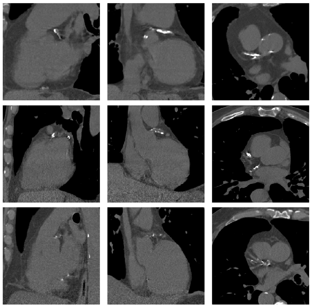
CAC examples, each row represent the patient heart bounding box, columns correspond to sagittal, coronal and axial plane. Bones and aorta calcifications have the same intensity range than CAC.

Fig. 2.

CAC Agatston Score normalized distribution on train, validation and test subsets. The Y axis is displayed in logarithmic scale to improve representation.

TABLE I.

CAC risk group samples distribution in train, validation and test subsets.

	Group 0	Group 1	Group 2	Group 3	Group 4	Total
Train	1920	1064	984	492	203	4663
Validation	206	114	106	53	21	500
Test	407	226	209	104	42	988

Fig. 3.

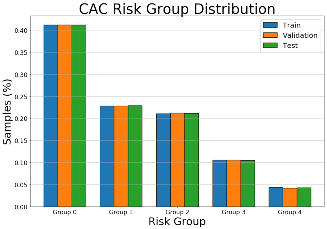
CAC risk group sample proportion plot.

Fig. 7.

Reference standard segmentations of the pectoralis muscle (blue) and subcutaneous fat (orange) for different patients.

Fig. 5.

PMA normalized distribution on the train, validation and test subsets.

Fig. 6.

SFA normalized distribution on the train, validation and test subsets.

B. Simultaneous biomarker and localization method

In this work, we propose a deep learning regression network able to regress the biomarker and to generate a mask from which the biomarker is generated. This has strong similarities to a segmentation problem, but instead of having segmentation masks for training, we use the value of the area or volume of the structure that is measured as the biomarker.

Inspired by this intuition, we propose the network of Fig. 1. The input image follows two paths of analysis. The first path consists of a set of rough segmentation operations to generate a mask of candidate points. Such mask should be highly sensitive to the pixels or voxels of the structure, even if it is non-specific. In this work, we have used a simple threshold operation, since muscle can be found in the range between [−20, 100], fat between [−140, −70] and coronary artery calcifications between [−500, 3000], however, more sophisticated methods could have been used. This mask serves as a pre-selection of the pixels or voxels that are aggregated to compute the biomarker.

The input image is also analyzed by a deep neural network that follows the structure of traditional segmentation networks, as the U-Net, a SE-Net, or a SD-Net. This is the network that is trained, but, unlike segmentation networks, we do not use segmentation masks for training. Instead, its output is multiplied by the mask of candidate points and input to a rectified linear unit to generate the localization mask. The localization mask is aggregated through a summation operation to generate the biomarker. The value of this biomarker is compared against the reference standard, and the error used to train the network.

The loss function used to train the network is the squared error between the estimated biomarker and the biomarker value ${\mathcal{L}}_2(y,\widehat{y})$ where ŷ represents the biomarker value, y represents the estimated biomarker.

The proposed method is agnostic with respect to the network structure of choice. To demonstrate this characteristic, we implemented our approach with three different segmentation networks: a U-Net structure [28], the Squeeze & Excitation modified version, SE-Net, explained in [29], and the SD-Net [30]. The SD-Net combines the U-Net Skip connections and the passing of indices for unpooling operations as it is used in the DeconvNet proposed for [31]. The last network has a significant limitation that consists in the obligation to have the same number of kernels in all convolutional layers in both, encoding and decoding part, avoiding keep the same trainable parameters in each level. Depending on the dimensionality of the regression problem, the network internal operations will be 2D or 3D. Please note that since there is no available implementation of the max-pooling with indices and unpooling operations in their 3D versions required for SD-Net, we discarded this network for CAC study.

The details of the network structures used in this work are as follow:

1. 2D U-Net: U-Net architecture [28] is composed of four encoding blocks consisting of two convolutions with a 3 × 3 kernels follow by a max-pooling operation of size 2. The number of convolution kernels increases as the network descends in-depth, with 32, 64, 128, 256 kernels in each level. Two more convolution layers, both with 512 (3 × 3) kernels, are performed in the inner level before the decoding part. The decoder is composed of four Up-sampling and convolution blocks, where the input of the last encoder layer is first resized with an up-sampling operation of size 2. A convolution layer with 2 × 2 kernels is applied before concatenating its output to the output of the encoder block at the same level. Then, two last convolutions with 3 × 3 kernels are performed. As the opposite of the encoder part, the number of convolutional kernel increase from 256 in the inner layer to 128, 64, and 32. All convolutions use a ReLU activation function and batch normalization. To finish, a last 1 × 1 single kernel convolution with sigmoid activation ensures the output is in the range [0, 1].

2. 2D SE-Net: Squeeze and Excitation Network (SE-Net) follows the same structure as U-Net with the addition of the scSE blocks, defined in [29], before the pooling operations of the encoder and after each decoder up-sampling blocks. This scSE operation is the result of the addition of two different computation paths. The first computes the global average pooling of the input, followed by two dense layers, one with half of the units that channels have the input and ReLU activations, and the other with the same units that channels, to keep the amount of data, with a sigmoid activation. Then, the output of the last dense layer is multiplied by the input data; this works as channel Weighing by relevance giving those who contribute the most a greater influence. The second computation path consists of a single 1 × 1 and one kernel convolution with a sigmoid activation, multiplying its output by the input data for performing a spatial weighing.

3. 2D SD-Net: Skip Deconvolution Networks [30] differs significantly in terms of layers composition. Although it maintains the appearance of an encoder-decoder, it uses an unpooling operation where the generated output is a reconstruction from a low-level data representation in conjunction with the indexes form where the data was obtained in the encoder pooling operation. In contrast to the traditional U-Net, this kind of network keeps the same number of convolutional kernels across all the network levels, 128 in this case. This is necessary to be able to use the unpooling operation with the indexes extracted from the encode pooling operations. As a summary, the network is composed of three encoder blocks, which consist of two convolution operations with 3 × 3 kernels and one max pooling layer that returns both the output and the indices from which it comes. In the inner part of the network, two convolutions are performed with the same kernel shape. The decoder part consists of three decoder blocks composed of the unpooling operation using indices extracted from the encoder same level block, followed by a convolution layer, the concatenation of the same level encoder output and two more convolution layers. All operations use a ReLU activation function. To finish, a last 1 × 1 single kernel convolution with sigmoid activation ensures the output is in the range [0,1].

4. 3D U-Net: The 3D version of the U-Net follows the same structure of the original 2D implementation but using 3 × 3 × 3 3D convolutional kernels instead of the originals 3 × 3. The number of kernels remains the same across all levels, as well as the activation types.

5. 3D SE-Net: Like happens with the U-Net, the 3D SE-Net keeps the same number kernels and activation types as its 2D version. Exchanging the kernels for their 3-dimensional version.

C. Computation of the Agatston score

The Agatston score, due to its non-linear relationship to image intensity, cannot be directly computed as the area or volume of structures of interest. Instead, a post-processing method of the localization mask is generated to obtain it from the localization mask using the formula described in [12]. The CAC computation consists of quantifying each connected component blob separately by taking each axial slice of the output localization volume and multiply by a factor based on the highest value of intensity by its area, finishing with the summation of all these values for computing a final aggregated biomarker. Please note that since the description of the original method developed by Agatston was designed to scans of fixed axial spacing resolution of 3mm we must adapt the computation multiplying the final value by a normalization factor.

D. Baseline methods

As baseline, three regression networks based in the encoding part of the network structures cited above were used, extracted from the remove of decoding blocks of the different network structures described in Section II-B. Two fully connected layers of 512 units with ReLU activation and one linear activated unit were added at the output of the networks to perform the regression task. Besides, for the CAC problem, we implemented the structure defined in previous work of [2] that consist of a simple encoder composed of three convolution-max-pooling blocks. The loss function used in all this baseline implementations is the mean absolute error (MAE), since it obtained the best performance in the regression networks loss comparison results of [32].

E. Training

The networks were trained separately over the different training sets, using the validation datasets to evaluate the performance at each training iteration. Early stopping criteria were used, which consisted of a basic convergence check over the validation loss, keeping the best model for testing purposes. The training learning rate was fixed in 1e⁻⁴, using an Adam optimizer with standard parameters.

Data augmentation was used due to the strong data imbalance present on the datasets (See Figs. 2, 5 and 6). For the CAC problem, the data augmentation technique used consisted of generating random displacements over the three axes, using a spherical probabilistic volume. This is done to ensure that the new augmented sample is equidistant from the center of the heart in all directions. The data augmentation is done on-the-fly, and to ensure reproducibility, the random seed of the data augmentation policy is fixed. Random rotations and translations were performed for the other two problems.

F. Evaluation metric

All metrics were calculated using the test dataset in each problem, which was used only to report the results of Table II.

TABLE II.

Results table, performance of the different networks that have been tested for this study, divided into two main sections. The left-hand side, labeled “Regression Networks”, contains the results of the reference methods. The right-hand side, entitled “Regression and Localization Networks”, displays the results of the proposed simultaneous biomarker regression and localization. Each row represents one of the proposed problems (PMA, SFA or CAC). Each column is the performance of the chosen network on the problems. ρ and ICC are reported for all networks. For PMA and SFA we also report the dice coefficient d and the average Hausdorff distance dH, since reference segmentation masks for the test set are available. For the problem of CAC, we also report the weighted kappa coefficient k and the accuracy for the different risk groups.

	Encoder Regression Networks				Regression and Localization Networks
	Baseline	Enc(U-Net)	Enc(SE-Net)	Enc(SD-Net)	RL-U-Net	RL-SE-Net	RL-SD-Net
PMA	ρ = 0.951 ICC = 0.950	ρ = 0.970 ICC = 0.969	ρ = 0.971 ICC = 0.967	ρ = 0.965 ICC = 0.963	ρ = 0.977 ICC = 0.976 d = 0.853 dH = 6.422	ρ = 0.978 ICC = 0.977 d = 0.875 dH = 7.049	ρ = 0.971 ICC = 0.970 d = 0.816 dH = 6.893
SFA	ρ = 0.971 ICC = 0.970	ρ = 0.982 ICC = 0.981	ρ = 0.982 ICC = 0.982	ρ = 0.981 ICC = 0.980	ρ = 0.998 ICC = 0.998 d = 0.914 dH = 5.857	ρ = 0.997 ICC = 0.997 d = 0.908 dH = 6.016	ρ = 0.996 ICC = 0.996 d = 0.817 dH = 7.147
CAC	ρ = 0.920 ICC = 0.919 κ = 0.761 acc = 0.780	ρ = 0.936 ICC = 0.926 κ = 0.727 acc = 0.726	ρ = 0.931 ICC = 0.931 κ = 0.753 acc = 0.750		ρ = 0.948 ICC = 0.946 κ = 0.853 acc = 0.885	ρ = 0.950 ICC = 0.950 κ = 0.852 acc = 0.842

The evaluation metrics were chosen depending on the particular problem and the availability of reference standard masks. All regressions were evaluated using Pearson correlation coefficient (ρ) and Inter-Class Correlation (ICC). For the PMA and SFA problems, the Dice coefficient (d) and Hausdorf distance (dH) to evaluate Image-based Biomarker localization performance. For the CAC problem, the regression values are often discretized in the following risk groups: [0,10), [10,100), [100,400), [400,1000) and 1000+. We have also computed the weighted kappa (κ) and accuracy (acc) for the categorical analysis.

G. Statistical analysis

To compare statistically two regression models against the reference standard, we employed Williams’s method [33]. The samples are not statistically independent since both regression models are tested on the same subjects, having the same reference method. William’s test takes into account the correlation coefficient between the reference standard and the first and second methods, as well as the correlation between both methods to establish a level of significance for the rejection of the null hypothesis. We establish the limit of statistical significance at p < 0.05. p-values lower than such limit reject the null hypothesis.

To test if the Dice scores come from the same distributions, we used the Kruskal-Wallis statistical method. Upon rejection of the null hypothesis, we perform a non-parametric comparison for all pairs of methods using the Dunn method for joint ranking. We repeat such analysis for the Haussdorf distances. Statistical analysis was performed with python’s scipy.stats and scikit-posthocs libraries. The limit of statistical significance is set at p < 0.05

To compare the confusion matrix for CAC group risk assignment from different regression methods, we use the Stuart-Maxwell test [34]. Statistical significance is set at p < 0.05 (Table IV).

TABLE IV.

Stuart-Maxwell test results comparing risk groups assignments between the different network structures used.

		Regression Networks (RN)			Regression and Localization Networks (RLN)
		baseline	Enc(U-Net)	Enc(SE-Net)	RL-U-Net	RL-SE-Net
RN	baseline	-	χ = 51.085 p – value = 2.143e – 10	χ = 16.56 p – value = 0.002353	χ = 49.319 p – value = 5.01e – 10	χ = 27.545 p – value = 1.542e – 05
	Enc(U-Net)	-	-	χ = 104.73 p – value < 2.2e – 16	χ = 147.47 p – value < 2.2e – 16	χ = 96.83 p – value < 2.2e – 16
	Enc(SE-Net)	-	-	-	χ = 31.143 p – value = 2.862e – 06	χ = 38.261 p – value = 9.897e – 08
RLN	RL-U-Net	-	-	-	-	χ = 65.152 p – value = 2.39e – 13

III. Results

A. Regression performance comparison

1. Performance of the regression networks: First, we evaluate the regression networks we have trained to obtain a reference to which compare the proposed method. Focusing on the baseline regression networks, more complex encoder networks structures like Enc(U-Net(E)), Enc(SE-Net(E)) or Enc(SD-Net) reach better regression performance. Specifically, PMA gets a Pearson correlation (ρ) of 0.951 for baseline in contrast to the 0.970 with Enc(U-Net), 0.971 of the Enc(SE-Net), or the 0.965 that is obtained using Enc(SD-Net). The differences in ρ with respect to the baseline are all statistically significant as shown in Table III. Similar results are obtained for SFA, with ρ of 0.971, 0.982, 0.982 and 0.981 respectively, all statistically significant with respect to the baseline (Supplementary material Table I). Finally, CAC correlation went from 0.920 for the baseline to 0.936 in Enc(U-Net) and 0.931 for the Enc(SE-Net), reaching again statistical significance with respect to the baseline (Supplementary material Table II).

2. Performance of simultaneous regression and localization methods: We have then compared the performance of the simultaneous regression and localization networks against that of the direct regression networks. Performance metrics for the simultaneous regression and biomarker localization networks are shown on the right-hand part of Table II. Correlation coefficients among pairs of equivalent network structures and problems favor the proposed method consistently. For the PMA problem, the regression network based on the Enc(U-Net) obtains a ρ coefficient of 0.970, while the proposed U-Net based regression and localization network (RL-U-Net) has a ρ of 0.977 (p < 0.05). The same network structure for SFA obtains ρ = 0.982 for Enc(U-Net) and ρ = 0.998 for RL-U-Net (ρ < 0.05). Similar results are obtained with respect to ρ for CAC: ρ = 0.936 for Enc(U-Net) and ρ = 0.948 for RL-U-Net (p < 0.05). There is a consistent improvement in the performance of the proposed networks with respect to the baseline, as can be seen in Table II. The same reasoning can be applied for the pairs of networks Enc(SE-Net) - RL-SE-Net and Enc(SD-Net) - RL-SD-Net.

   Figs. 8 and 9 display Bland-Altman analysis and correlation plots for the PMA and SFA and CAC problems respectively using the RL-SE-Net. In all three cases, we observe that there is no systematic error since the Bland-Altmann analysis is centered around 0. Errors seem to be constant for all ranges of values in all three cases. Some outliers are present on the Bland-Altman analysis and are analyzed in detail in the supplementary material.

3. Regression dependency on network structure: The results shown in Table II demonstrate that the regression performance of the proposed regression and localization networks does not vary much with respect to the network structure that is being used as backbone.

   Focusing on PMA, the ρ coefficients are of 0.977, 0.978 and 0.971 for the RL-U-Net, the RL-SE-Net, and the RL-SD-Net respectively, showing a small but statistically significant discrepancy (p-values between the RL-U-Net and the RL-SE-Net is < 0.05; between the RL-U-Net and the RL-SD-Net is < 0.05 and between the RL-SD-Net and the RL-SE-Net is also < 0.05) as shown in Table III. The same results appear in the problem of SFA, with ρ coefficients of 0.998, 0.997 and 0.996 for the RL-U-Net, the RL-SD-Net and the RL-SE-Net respectively. The difference between RL-U-Net and RL-SE-UNet is not statistically significant (p = 0.41), as shown in supplementary materials Table I, while between the other two networks, the p-values are lower than < 0.05.

   For the problem of CAC, the two networks analyzed have very similar ρ, being it of 0.948 for the RL-U-Net and 0.950 for the RL-SE-Net. These two networks did not reach statistical significance (p = 0.765), as shown in supplementary material Table II.

TABLE III.

Results of the statistical tests performed between all pairs of networks for the pectoralis muscle area problem. p_c, p_d, and PdH stand for the p-values for the regression, the DICE measurements, and the Haussdorf distances, computed as explained in SECTION II-G. P-values that do not reach the level of significance of 0.05 are shown in red. A similar table for the subcutaneous fat and coronary artery calcifications are included in the supplementary material due to space limitations.

		Regression Networks (RN)			Regression and Localization Networks (RLN)
		Enc(U-Net)	Enc(SE-Net)	Enc(SD-Net)	RL-U-Net	RL-SE-Net	RL-SD-Net
RN	baseline	pc < 0.05	pc < 0.05	pc < 0.05	pc < 0.05	pc < 0.05	pc < 0.05
	Enc(U-Net)	-	pc < 0.05	pc < 0.05	pc < 0.05	pc < 0.05	pc = 0.87
	Enc(SE-Net)	-	-	pc < 0.05	pc < 0.05	pc < 0.05	pc < 0.05
	Enc(SD-Net)	-	-	-	pc < 0.05	pc < 0.05	pc < 0.05
RLN	RL-U-Net	-	-	-	-	pc < 0.05; pd, pDH < 0.05	pc, pd, pDH < 0.05
	RL-SE-Net	-	-	-	-	-	pc, pd < 0.05; pdH < 0.05

Fig. 8.

PMA result plots (top) and SFA (bottom) using SE-Net and U-Net respectively as proposed method cores. From left to right: Bland-Altman, correlation and biomarker localization output where each sample have a colored dot than correspond with the same in the correlation plot. Also, the localization is depicted using three colors for True positives (Green), False Positives (Yellow) and False Negative (Red). The grey structure shows the candidate mask where biomarker should be found.

Fig. 9.

CAC results using the proposed method over a U-net network. Left to Right: Bland-Altman, correlation plot and risk groups confusion matrix.

B. Structure localization dependency on network structure

Since the masks for the testing data of pectoralis muscle and subcutaneous fat were available, we can compute the Dice coefficient and the Hausdorff distance of the localization masks.

Quantitative analysis is shown in Table II. For the pectoralis muscle area, we achieve DICE coefficients of 0.853, 0.875, and 0.816 for the RL-U-Net, RL-SE-Net and RL-SD-Net based proposed networks respectively, all pairs statistically significantly different, as shown on Table III. Similarly, for subcutaneous fat, the proposed method achieves DICE coefficients of 0.914, 0.908 and 0.817 for the RL-U-Net, RL-SE-Net and the RL-SD-Net backbones, also statistically significantly different. It is important to see that while the RL-SD-Net’s regression performance does not differ much to the alternatives, its dice coefficient is much lower. This might be due to the small number of kernels that such networks have on their layers and suggest that the SD-Net is not a good network choice for biomarker localization.

Comparing these results with those obtained by the CUNet proposed in the work of [35], we found that our method gets similar localization performance for both, Pectoralis Muscle and Subcutaneous Fat. In terms of mean per-and Subcutaneous Fat. In terms of mean per-class Dice Score, the proposed method obtains a 0.895 vs. the 0.916 using CUNet network.

The mean Hausdorff distance between the proposed method and the reference standard for PMA is 6.42, 7.05, and 6.89 pixels for the RL-U-Net, RL-SE-Net, and RL-SD-Net respectively, all pairs statistically significant with p < 0.05. For SFA, mean Hausdorff distance is 5.86, 6.02, and 7.15 (p < 0.05 for all pair-wise comparisons). While the RL-U-Net and the RL-SE-Net perform similarly concerning dice coefficients, these results show that the RL-U-Net has a lower Hausdorff distance consistently to the reference standard, generating better localization masks.

Examples of the localization obtained for six equally spaced cases for PMA and SFA are shown in Fig. 8. On them, we show true positives in green, false positives in yellow and false negatives in red. The localization voxels are overlaid over the candidates’ mask (in gray). In other words, gray pixels are potential candidates for the biomarker localization, and the network learns which pixels belong to the structure by looking only at the biomarker value. Besides, Fig. 11 shown the inferred voxels from where the Agatston score is measured, note that the system discards other structures like bones and calcification plaques in the aorta. As we can see, the method is robust with respect to the size of the structure and the variability of the number of candidate voxels, showing considerable agreement with the reference standard.

Fig. 11.

CAC biomarker localization obtained by the proposed method using a U-Net structure as basis. Green regions represent the calcifications founded in the coronary arteries, note that calcifications in the aorta and bones was discarded by the network.

C. Risk accuracy in Agatston score computation

The problem of Agatston score computation offers further opportunities for evaluation. As mentioned in the introduction, the Agatston score is discretized in risk groups to estimate the risk of the patient having a cardiovascular event. Such discretization allows us to compare the performance of the regressed Agatston score value against the risk-group reference standard. Such confusion matrix is displayed in Fig. 9. To quantify the performance of the risk-group categorization, we resort to the κ metric, which is displayed in Table II. We can see that the proposed regression and localization networks obtain a κ value of 0.85, for both the RL-U-Net and the RL-SE-Net. Please compare these numbers with the performance of the direct regression networks, that obtain the values of κ of 0.76, 0.73 and 0.75 for the baseline, the Enc(U-Net) and the Enc(SE-Net) based regressors respectively. Similar metrics are obtained for the risk-accuracy, where the proposed method classifies a subject in the correct risk group with 88.5% accuracy, while the baseline method does so 78% of the times. An example of the confusion matrix is shown in Fig. 9.

The κ values of the proposed methods are comparable to the state of the art, getting close to those obtained in the recent work of [5], where they obtained a κ value of 0.93 and a risk-accuracy of 0.90 using Chest CT.

Unfortunately, it has not been possible to test CAC on a SD-Net due to implementation limitations, since the pooling and unpooling operations with indexes in 3D are not available in the Keras or the TensorFlow libraries and their implementation proved to be non-trivial.

While we do not have a reference standard with whom to test the performance of the CAC localization masks, it is essential to note that the correlation figures shown in this section correlate with the quality of the localization masks. Indeed, as explained in material and methods, the Agatston score is computed from the localization masks. When training the simultaneous localization and regression network, we optimize for the volume of the coronary arteries lesion. After network convergence, we compute the Agatston score from the localization mask obtained with our method. Therefore, the high correlation we obtain in the Agatston score computation is due to the correct localization and delineation of the lesions in the images. Examples of such localization masks are displayed in Fig. 4.

D. Liver tumor regression and localization, comparison to a segmentation network

Fig. 12 shows qualitative results of the application of the RL-U-Net to the problem of liver tumor size regression and localization. For three different cases, we show the axial slice where the tumors are present, the result of the RL-U-Net and the result of applying a baseline U-Net segmentation. Such baseline network has the same structure as the backbone network used for the RL-U-Net. True positives are shown in green, false positives in red and false negatives in yellow. We can see comparable qualitative results between both networks.

Fig. 12.

Liver tumor localization comparing the proposed method with the traditional segmentation method using a U-Net. Green, Red and Yellow regions means the True Positives, False Negatives and False Positive, respectively.

Quantitatively, on a per-case basis, the RL-U-Net achieved a Pearson correlation coefficient of 0.989, while the U-Net achieved a correlation coefficient of 0.951 (p < 0.05). Pearson correlation coefficients on a per-slice basis are of 0.931 for RL-U-Net and 0.876 for U-Net (p < 0.05). When performing regression, the proposed method outperforms the U-Net segmentation network significantly.

When comparing the Dice coefficients of the localization network and the reference standard vs. the dice coefficients of the U-Net, the results favor the segmentation network trained with the segmentation masks. The average Dice coefficients per slice for the U-Net are of 0.576 vs. 0.532 of the RL-U-Net (p < 0.05). When analyzing complete scans, the U-Net achieved an average score of 0.699 and the RL-U-Net of 0.617. Probably due to the small number of data points, 18 scans, the Kruskal-Wallis test did not pass, and therefore the null hypothesis can not be rejected for this pair of measurements.

E. Number of required training samples

To research how many samples are required to train the proposed method, we have trained the U-Net based simultaneous regression and localization network for the problems of PMA, SFA and CAC with various numbers of training samples. We have performed five repeats for each problem and each number of training samples. As one could expect, the performance, both in terms of ρ and of Dice coefficient improves with the number of training samples. However, there is a sharp increase until approximately 1000 training samples. The methods plateau after such number, showing a moderate increase, as shown in Fig. 13. It is important to note that the variance of the performance decreases with the number of training samples, as could be expected.

Fig. 13.

Performance progression for different amount of train samples. CAC is measured in biomarker correlation coefficient. PMA and SFA in both, biomarker correlation and localization dice coefficient. We tested the system using 300, 500, 1000, 2000, 4000 and 5000 training samples for a total of 5 times for each problem and number of samples used. Each line represents the mean, maximum and minimum values and its standard deviation.

IV. Discussion

The proposed simultaneous biomarker regression and localization network has proven to regress biomarkers better than the direct regression networks, as shown in Table II, while simultaneously obtaining the biomarker localization mask. Indeed, we have re-formulated the problem of biomarker regression, instead of mapping an image to a real value, we find the subset of voxels in the image that form the area or volume of the biomarker, and then adding such voxels to generate the biomarker to which we perform the regression.

There are two potential reasons why the proposed network outperforms direct regression networks. The first one is network complexity. The proposed method uses a full encoder-decoder architecture with skip connections, which enables both local and global features to be taken into account to compute the biomarker. However, it is the shift of the paradigm and the hybrid cost function that enables the use of such network structures. The second reason could be that we are providing the network with extra expert knowledge of the problem when generating the candidates’ masks. While such is a valid reason, the simplicity with which the candidates’ mask is generated (a simple threshold followed optionally by morphological operations) means that it could be easily trained. Indeed, such an option remains for future research, as well as to analyze the influence of such candidates’ regions on the whole system.

Other approaches postulate the use of attention maps to define the regions where the network is focusing on. They employ a variety of methods ranging from the use of Attention Gates (AG) to highlight the regions where a network is focusing [36], computing an aggregated score map directly from the feature vectors of the intermediate representation at different network levels [37] or using decovolutional networks [38] to visualize the regions in an image that contributes most to the output [5]. The main difference between such work and ours is that they require either network architecture modifications after training or their localization masks are low-resolution, requiring some post-processing methods to obtain more accurate biomarker localization. In contrast, our method does not need any post-processing modification to get an original full resolution localization map.

We have shown how the method generalizes with respect to the backbone network used, as demonstrated by the experiments using the U-Net, the SE-Net and the SD-Net. Even though these networks share the same encoder-decoder structure, we hypothesize that our training methodology could be used with other segmentation networks, as long as they generate an image of the same resolution as the input. We have also shown the generalization of the proposed method with respect to the segmentation problem, using the 2D computation of pectoralis muscle area, subcutaneous fat area, and the 3D computation of the Agatston score as the problems of choice. Clearly, the performance changes with the complexity of the problem, but so does the performance of regular regression networks.

Localization results obtained must be analyzed more deeply. Dice coefficients show a high agreement with the reference standard, but we must be aware that these references have a subjective component, which may mean that both reference standard and our method outputs, represent a valid structure location. If we compare a typical segmentation network with our proposed method version, the latter one grants a new freedom dimension in the way we are not limited the network to learn based on a subjective delimited reference segmentation mask, but also training with only the biomarker value, giving the network a larger margin to infer the localization of the structure within the known candidate regions.

Focusing on the biomarker regression of the Agatston score, our method produces an Inter Class Correlation coefficient (ICC) of 0.95 using non ECG-Gated chest CT. Such coefficient is close to state-of-the-art methods. For example, the work of [5] obtain an ICC of 0.97 in Agatston score direct regression, close to the 0.96 obtained by [39], both using ECG-Gated cardiac CT, which are often images of higher quality. One may claim that, in comparison with other works, we have compensated image quality by the use of a much larger dataset. The experiments in Fig. 13 related to the number of training samples allow us to conclude that with 1500 training scans, the system is able to find a suitable solution, even though the system variability remains fairly high. Such number, 1500 training samples, is not a large difference in comparison of the 1239 Cardiac+Chest CT or the 1013 Cardiac CT used respectively in the works cited above.

To further show the generality of the proposed method, we have applied it to the regression of liver tumor area and compared it against a reference u-net segmentation network. The proposed method achieved a better correlation coefficient to the reference standard than the segmentation method. However, the Dice coefficient between the segmentation u-net and the proposed network favored the segmentation network. Such is of little surprise, since the segmentation network uses segmentation masks for training, while the proposed method does not. Further, the Dice coefficient is not linear with respect to the number of pixels or voxels that are misclassified; it all depends on the number of pixels that the reference segmentation has. As such, an error if 1 pixel can generate a dice score of 0 if the reference mask has a 1-pixel size, or have almost no influence if the reference mask has 100 pixels. This property leads to the optimization of the segmentation network towards small areas. In contrast, when performing regression and using the ${\mathcal{L}}_2$ norm for optimization, one misclassified pixel has the same influence on whether the reference label is of 1 pixel or 100 pixels. This property leads to better performance on regression of the proposed method while having a lower performance on segmentation matrices.

A. Limitations

The main limitation is that the proposed method can only be applied to biomarkers that can be measured as an area, a volume, or that can be computed from a localization mask by applying some transformation. While many biomarkers fall in this category, regression networks are not only limited to such types of biomarkers and could infer, for instance, spirometry data from the images.

A second limitation is that the regression values come from manual annotations, and to obtain such values, a segmentation should have been made. Therefore, why not using the segmentation in the first place? We were inspired by the CAC dataset, a large dataset generated for a clinical study to which no segmentation was saved. We believe this dataset is not unique to its kind, and that similar datasets can be extracted from clinical practice. As an example, the RECIST criteria for the evaluation of tumor progression.

V. Conclusion

We have presented a method that not only improves the regression performance in comparison with the normal regression networks, but also returns an image-based biomarker localization map as a direct by-product of the regression computation without applying any post-processing task like switching layers or attention methods. The proposed method does not need any reference segmentation for training. We have shown that the proposed method can use any encoder-decoder segmentation network as backbone and that it is applicable to different 2D and 3D regression problems, achieving state-of-the-art performance.

Fig. 10.

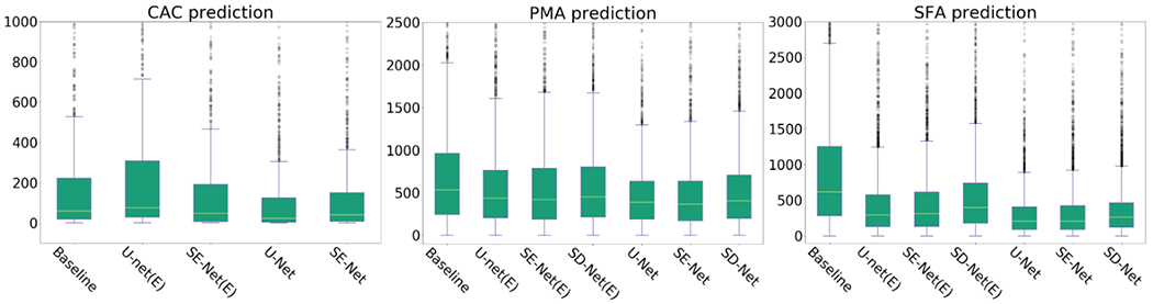
Box plot comparison between baseline regression methods and proposed method.

References

- [1].Strimbu K and Tavel JA, “What are biomarkers?” Current Opinion in HIV and AIDS, vol. 5, no. 6, p. 463, 2010. [DOI] [PMC free article] [PubMed] [Google Scholar]
- [2].Cano-Espinosa C, González G, Washko GR, Cazorla M, and San José Estépar R, “Automated agatston score computation in non-ecg gated ct scans using deep learning,” in Medical Imaging - Image Processing-Proceedings of SPIE, no. March, 2018. [DOI] [PMC free article] [PubMed] [Google Scholar]
- [3].González G, Washko GR, and San José Estépar R, “Deep learning for biomarker regression : application to osteoporosis and emphysema on chest CT scans,” in Medical Imaging - Image Processing-Proceedings of SPIE, no. March, 2018b. [DOI] [PMC free article] [PubMed] [Google Scholar]
- [4].Dubost F, Bortsova G, Adams H et al. , “Gp-unet: Lesion detection from weak labels with a 3d regression network,” in International Conference on Medical Image Computing and Computer-Assisted Intervention. Springer, 2017, pp. 214–221. [Google Scholar]
- [5].de Vos BD, Wolterink JM, Leiner T, de Jong PA, Lessmann N, and Išgum I, “Direct automatic coronary calcium scoring in cardiac and chest ct,” IEEE transactions on medical imaging, 2019. [DOI] [PubMed] [Google Scholar]
- [6].Yan C, Yao J, Li R, Xu Z, and Huang J, “Weakly supervised deep learning for thoracic disease classification and localization on chest xrays,” in Proceedings of the 2018 ACM International Conference on Bioinformatics, Computational Biology, and Health Informatics. ACM, 2018, pp. 103–110. [Google Scholar]
- [7].Long J, Shelhamer E, and Darrell T, “Fully convolutional networks for semantic segmentation,” in The IEEE Conference on Computer Vision and Pattern Recognition (CVPR), June 2015. [DOI] [PubMed] [Google Scholar]
- [8].Kinsey CM, San José Estépar R, Van der Velden J, Cole BF, Christiani DC, and Washko GR, “Lower pectoralis muscle area is associated with a worse overall survival in non–small cell lung cancer,” 2017. [DOI] [PMC free article] [PubMed] [Google Scholar]
- [9].McDonald M-LN, Diaz AA, Ross JC, San José Estépar R, Zhou L, Regan EA, Eckbo E, Muralidhar N, Come CE, Cho MH et al. , “Quantitative computed tomography measures of pectoralis muscle area and disease severity in chronic obstructive pulmonary disease. a cross-sectional study,” Annals of the American Thoracic Society, vol. 11, no. 3, pp. 326–334, 2014. [DOI] [PMC free article] [PubMed] [Google Scholar]
- [10].Harmouche R, Ross JC, Washko GR, and San José Estépar R, “Pectoralis muscle segmentation on ct images based on bayesian graph cuts with a subject-tailored atlas,” in International MICCAI Workshop on Medical Computer Vision. Springer, 2014, pp. 34–44. [Google Scholar]
- [11].Moreta-Martinez R, Onieva-Onieva J, Pascau J, and San José Estépar R, “Pectoralis muscle and subcutaneous adipose tissue segmentation on ct images based on convolutional networks.” Springer, 2017. [Google Scholar]
- [12].Agatston AS, Janowitz WR, Hildner FJ, Zusmer NR, Viamonte M, and Detrano R, “Quantification of coronary artery calcium using ultrafast computed tomography,” Journal of the American College of Cardiology, vol. 15, no. 4, pp. 827–832, 1990. [DOI] [PubMed] [Google Scholar]
- [13].Budoff MJ, Nasir K, Kinney GL, Hokanson JE, Barr RG, Steiner R, Nath H, Lopez-Garcia C, Black-Shinn J, and Casaburi R, “Coronary artery and thoracic calcium on noncontrast thoracic ct scans: comparison of ungated and gated examinations in patients from the copd gene cohort,” Journal of cardiovascular computed tomography, vol. 5, no. 2, pp. 113–118, 2011. [DOI] [PMC free article] [PubMed] [Google Scholar]
- [14].Wolterink JM, Leiner T, Takx RA, Viergever MA, and Išgum I, “An automatic machine learning system for coronary calcium scoring in clinical non-contrast enhanced, ecg-triggered cardiac ct,” in Medical Imaging 2014: Computer-Aided Diagnosis. International Society for Optics and Photonics, 2014, p. 90350E. [Google Scholar]
- [15].Shahzad R, van Walsum T, Schaap M, Rossi A, Klein S, Weustink AC, de Feyter PJ, van Vliet LJ, and Niessen WJ, “Vessel specific coronary artery calcium scoring: an automatic system,” Academic radiology, vol. 20, no. 1, pp. 1–9, 2013. [DOI] [PubMed] [Google Scholar]
- [16].Isgum I, Prokop M, Niemeijer M, Viergever MA, and van Ginneken B, “Automatic coronary calcium scoring in low-dose chest computed tomography,” IEEE transactions on medical imaging, vol. 31, no. 12, pp. 2322–2334, 2012. [DOI] [PubMed] [Google Scholar]
- [17].Xie Y, Cham MD, Henschke C, Yankelevitz D, and Reeves AP, “Automated coronary artery calcification detection on low-dose chest ct images,” in Proc. SPIE, vol. 9035, 2014, p. 90350F. [Google Scholar]
- [18].Wolterink JM, Leiner T, de Vos BD, van Hamersvelt RW, Viergever MA, and Išgum I, “Automatic coronary artery calcium scoring in cardiac ct angiography using paired convolutional neural networks,” Medical image analysis, vol. 34, pp. 123–136, 2016. [DOI] [PubMed] [Google Scholar]
- [19].Bray F, Ferlay J, Soerjomataram I, Siegel RL, Torre LA, and Jemal A, “Global cancer statistics 2018: Globocan estimates of incidence and mortality worldwide for 36 cancers in 185 countries,” CA: a cancer journal for clinicians, vol. 68, no. 6, pp. 394–424, 2018. [DOI] [PubMed] [Google Scholar]
- [20].Albain KS, Swann RS, Rusch VW, Turrisi AT III, Shepherd FA, Smith C, Chen Y, Livingston RB, Feins RH, Gandara DR et al. , “Radiotherapy plus chemotherapy with or without surgical resection for stage iii non-small-cell lung cancer: a phase iii randomised controlled trial,” The Lancet, vol. 374, no. 9687, pp. 379–386, 2009. [DOI] [PMC free article] [PubMed] [Google Scholar]
- [21].Rossi S, Di Stasi M, Buscarini E, Quaretti P, Garbagnati F, Squassante L, Paties C, Silverman D, and Buscarini L, “Percutaneous rf interstitial thermal ablation in the treatment of hepatic cancer.” AJR. American journal of roentgenology, vol. 167, no. 3, pp. 759–768, 1996. [DOI] [PubMed] [Google Scholar]
- [22].Chapiro J, Duran R, Lin M, Schernthaner RE, Wang Z, Gorodetski B, and Geschwind J-F, “Identifying staging markers for hepatocellular carcinoma before transarterial chemoembolization: comparison of threedimensional quantitative versus non–three-dimensional imaging markers,” Radiology, vol. 275, no. 2, pp. 438–447, 2014. [DOI] [PMC free article] [PubMed] [Google Scholar]
- [23].Regan E. a., Hokanson JE, Murphy, Lynch JR et al. , “Genetic Epidemiology of COPD (COPDGene) Study Design,” Epidemiology, vol. 7, no. 1, pp. 1–10, 2011. [DOI] [PMC free article] [PubMed] [Google Scholar]
- [24].González G, Washko GR, and San José Estépar R, “Automated agatston score computation in a large dataset of non ecg-gated chest computed tomography,” in Biomedical Imaging (ISBI) 2016 IEEE 13th International Symposium on. IEEE, 2016, pp. 53–57. [DOI] [PMC free article] [PubMed] [Google Scholar]
- [25].Rodriguez-Lopez S, Jimenez-Carretero D, San José Estépar R, Moreno EF, Kumamaru KK, Rybicki FJ, Ledesma-Carbayo MJ, and Gonzalez G, “Automatic ventricle detection in computed tomography pulmonary angiography,” in Biomedical Imaging (ISBI) 2015 IEEE 12th International Symposium on IEEE, 2015, pp. 1143–1146. [Google Scholar]
- [26].San José Estépar R, Ross JC, Harmouche R et al. , “Chest imaging platform: an open-source library and workstation for quantitative chest imaging,” in C66. LUNG IMAGING II: NEW PROBES AND EMERGING TECHNOLOGIES. American Thoracic Society, 2015, pp. A4975–A4975. [Google Scholar]
- [27].Bilic P, Christ PF, Vorontsov E, Chlebus G, Chen H, Dou Q, Fu C-W, Han X, Heng P-A, Hesser J et al. , “The liver tumor segmentation benchmark (lits),” arXiv preprint arXiv:1901.04056, 2019. [Google Scholar]
- [28].Ronneberger O, Fischer P, and Brox T, “U-net: Convolutional networks for biomedical image segmentation,” in International Conference on Medical image computing and computer-assisted intervention. Springer, 2015, pp. 234–241. [Google Scholar]
- [29].Roy AG, Navab N, and Wachinger C, “Concurrent spatial and channel ‘squeeze & excitation’in fully convolutional networks,” in International Conference on Medical Image Computing and Computer-Assisted Intervention. Springer, 2018, pp. 421–429. [Google Scholar]
- [30].Roy AG, Conjeti S, Sheet D, Katouzian A, Navab N, and Wachinger C, “Error corrective boosting for learning fully convolutional networks with limited data,” in International Conference on Medical Image Computing and Computer-Assisted Intervention. Springer, 2017, pp. 231–239. [Google Scholar]
- [31].Noh H, Hong S, and Han B, “Learning deconvolution network for semantic segmentation,” in Proceedings of the IEEE international conference on computer vision, 2015, pp. 1520–1528. [Google Scholar]
- [32].Cano-Espinosa C, González G, Washko GR, Cazorla M, and San José Estépar R, “On the relevance of the loss function in the agatston score regression from non-ecg gated ct scans,” in Image Analysis for Moving Organ, Breast, and Thoracic Images. Cham: Springer International Publishing, 2018, pp. 326–334. [DOI] [PMC free article] [PubMed] [Google Scholar]
- [33].Williams EJ, “The Comparison of Regression Variables,” Journal of the Royal Statistical Society: Series B (Methodological), vol. 21, no. 2, pp. 396–399, 1959. [Google Scholar]
- [34].Maxwell AE, “Comparing the classification of subjects by two independent judges.” The British journal of psychiatry : the journal of mental science, vol. 116, no. 535, pp. 651–655, 1970. [DOI] [PubMed] [Google Scholar]
- [35].González G, Washko GR, and San José Estépar R, “Multi-structure segmentation from partially labeled datasets. application to body composition measurements on ct scans,” in Image Analysis for Moving Organ, Breast, and Thoracic Images. Springer, 2018a, pp. 215–224. [DOI] [PMC free article] [PubMed] [Google Scholar]
- [36].Oktay O, Schlemper J, Folgoc LL, Lee M, Heinrich M, Misawa K, Mori K, McDonagh S, Hammerla NY, Kainz B et al. , “Attention u-net: Learning where to look for the pancreas,” arXiv preprint arXiv:1804.03999, 2018. [Google Scholar]
- [37].Jetley S, Lord NA, Lee N, and Torr PH, “Learn to pay attention,” arXiv preprint arXiv:1804.02391, 2018. [Google Scholar]
- [38].Zeiler MD, Taylor GW, Fergus R et al. , “Adaptive deconvolutional networks for mid and high level feature learning.” in ICCV, vol. 1, no. 2, 2011, p. 6. [Google Scholar]
- [39].Wolterink JM, Leiner T, Takx RA, Viergever MA, and Išgum I, “Automatic coronary calcium scoring in non-contrast-enhanced ecg-triggered cardiac ct with ambiguity detection,” IEEE transactions on medical imaging, vol. 34, no. 9, pp. 1867–1878, 2015. [DOI] [PubMed] [Google Scholar]
Associated Data
This section collects any data citations, data availability statements, or supplementary materials included in this article.