

Abstract
Untargeted metabolomics experiments provide a snapshot of cellular metabolism but remain challenging to interpret due to the computational complexity involved in data processing and analysis. Prior to any interpretation, raw data must be processed to remove noise and to align mass-spectral peaks across samples. This step requires selection of dataset-specific parameters, as erroneous parameters can result in noise inflation. While several algorithms exist to automate parameter selection, each depends on gradient descent optimization functions. In contrast, our new parameter optimization algorithm, AutoTuner, obtains parameter estimates from raw data in a single step as opposed to many iterations. Here, we tested the accuracy and the run-time of AutoTuner in comparison to isotopologue parameter optimization (IPO), the most commonly used parameter selection tool, and compared the resulting parameters’ influence on the properties of feature tables after processing. We performed a Monte Carlo experiment to test the robustness of AutoTuner parameter selection and found that AutoTuner generated similar parameter estimates from random subsets of samples. We conclude that AutoTuner is a desirable alternative to existing tools, because it is scalable, highly robust, and very fast (∼100–1000× speed improvement from other algorithms going from days to minutes). AutoTuner is freely available as an R package through BioConductor.
Metabolomics is the study of all the compounds present within a cell, organism, or tissue. Such investigations provide a holistic snapshot of the activity within a biological matrix and have led to a myriad of discoveries ranging from the elucidation of novel biochemical pathways to the recognition of molecular adaptive responses to stress and the clarification of mechanisms driving cell–cell interactions.1−3 Advances in mass spectrometry fostered these discoveries, specifically improvements in instrument sensitivity, accuracy, and data collection capacity.1,4,5 Parallel advances in computational tools have historically followed to fulfill the potential of analytical improvements.6
Prior to data analysis, raw data from untargeted metabolomics experiments must be processed to generate a features table. Features are defined as peaks with unique mass to charge (m/z) and retention time values, with relative abundances determined by their height or area. Processing is critical to extract chemical signals from electrical noise and to correct for retention time drift across samples.7 A variety of untargeted data processing methods exist,8−11 including two commonly used tools: MZmine212 and XCMS.13 Although these tools reliably extract true features from complex data, their performance depends on the selection of algorithmic parameters that capture the structure of the data, such as matrix effects and differences in analytical platforms.14−16 No universal set of parameters exists for all datasets; hence, parameter optimization must occur prior to analysis to avoid noise inflation within the feature table.17−19
Tuning parameters manually is prohibitively time-consuming due to the high number of possible numerical combinations. To overcome this challenge, several methods exist to identify optimal dataset-specific parameters.20−22 These methods each use distinct optimization functions based on maximizing or minimizing a numerical value. Each approach iteratively runs XCMS peak-picking and retention time correction algorithms until they identify a set of parameters that optimizes a desired criterion. For example, isotopologue parameter optimization (IPO), the most commonly used parameter selection tool, scores groups of parameters by the number of features detected after XCMS that contain a naturally occurring 13C isotopologue. Many separate XCMS runs are required to find ideal parameters, sometimes taking weeks to complete.20−22 Currently, these parameter selection algorithms depend on high performance computing resources. As users continue to adopt ultrahigh pressure liquid chromatography systems and rapid scanning mass spectrometers, the size and abundance of data from these platforms will preclude the use of unscalable parameter selection algorithms to users without access to high performance computing resources.23,24
We designed a novel parameter optimization algorithm, AutoTuner, to ameliorate these challenges. The method performs statistical inference on raw data in a single step in order to make parameter estimates as opposed to iteratively checking estimates. Further, it complements recent tools focused on generating higher-confidence feature annotations.25−28 AutoTuner is capable of selecting parameters for seven continuously valued parameters required for centWave peak selection algorithm used by both MZmine2 and XCMS, and it determines a key parameter for grouping in XCMS. AutoTuner is freely distributed through BioConductor as an R package.
Theory and Design of AutoTuner
Algorithm Overview
AutoTuner makes estimates for the following mass spectrometry peak-picking and grouping algorithms parameters: Group difference, parts per million (ppm), Signal to Noise (S/N) Threshold, Scan count, Noise, Prefilter intensity, and Minimum/Maximum Peak-width. We chose to optimize these parameters because they have the greatest influence on the number and quality of features postprocessing and have the greatest number of possible values.21,29 We chose to optimize centWave peak-picking parameters over other peak-picking methods, as centWave is the recommended method for processing high-resolution untargeted data, which is increasingly becoming the standard for untargeted metabolomics.4 See Table 1 for a description of the parameters and their matching arguments in XCMS. AutoTuner makes estimates in three steps ( Figure 1). (1) Total ion chromatogram (TIC) peak detection: A user identifies peaks within each sample’s total ion chromatogram (TIC), which is the plot of the integrated ion intensities within the mass spectrometer over time. (2) Parameter estimation within extracted ion chromatograms (EICs) of each TIC peak: AutoTuner isolates predicted EICs within each identified TIC peak. An EIC is a plot of one or more selected m/z values in a series of mass spectra. AutoTuner applies statistical inference on all EIC peaks to estimate parameters in an unsupervised manner. (3) Dataset-wide parameter estimates: AutoTuner integrates all peak-specific estimates into a dataset-wide set.
Table 1. Parameters Estimated through the AutoTuner Algorithma.
| parameter | description | XCMS parameter name | functionality | application |
|---|---|---|---|---|
| Group difference | expected retention time deviation of an mz/rt feature between samples | bw | grouping | XCMS |
| ppm | parts per million (ppm) error threshold used to bin consecutive mass intensities across adjacent scans into a single peak | ppm | centWave (peak-picking) | XCMS and MZmine2 |
| S/N Threshold | the minimum ratio between peak and average noise intensity required to retain a feature | snthresh | centWave (peak-picking) | XCMS and MZmine2 |
| Scan count | minimum number of scans required to retain a peak | prefilter scan | centWave (peak-picking) | XCMS and MZmine2 |
| Noise | numerical threshold used to filter out noise from true masses | noise | centWave (peak-picking) | XCMS and MZmine2 |
| Prefilter intensity | minimum integrated intensity required retain a peak | prefilter intensity | centWave (peak-picking) | XCMS and MZmine2 |
| Peak-width | the width of a chromatographically resolved peak | min/max peak-width | centWave (peak-picking) | XCMS and MZmine2 |
Figure 1.

Schematic of the three stages of the AutoTuner algorithm. (A) Total ion chromatogram (TIC) peak detection requires user input and is focused on identifying peaks within each sample’s TIC. The user directly adjusts a signal processing sliding window analysis to identify peaks within the TIC. (B) Parameter estimation within extracted ion chromatograms (EICs) of each TIC peak iteratively looks at each peak to make parameter estimates from EICs. (C) Data set-wide parameter estimates aggregate results from the second stage to provide an ideal set of parameters for the entire dataset. Parameters estimated are in bold. The R package vignette at BioConductor provides an example on how to use the algorithm.
Total Ion Chromatogram (TIC) Peak Detection
To identify TIC peaks, AutoTuner first applies a sliding window analysis, which detects peaks by testing if an upcoming scan’s intensity is greater than an intensity threshold determined by the average and standard deviation of a fixed number of prior scans. To ensure the correct peak bounds are retained, AutoTuner generates a linear model from the first three and last three points bounding each TIC peak. If the model fails to calculate an R2 value greater than or equal to 0.8 or to reach a local R2 maximum, AutoTuner expands the ending bound by one scan and reruns the model until the model meets either criterion. The time difference of a TIC peak’s final bounds represents its width.
AutoTuner groups all TIC peaks originating from distinct samples whose maxima co-occur within each other’s retention-time bounds. It then determines the time differences between intensity maxima of all pairs of grouped peaks. AutoTuner returns the largest time difference as the estimate for the Group difference parameter that is used in the grouping step following peak-picking. Because highly complex datasets may contain distinct sample-specific peaks occurring at similar retention times, AutoTuner may overestimate this parameter. Prioritizing the inclusion of experimental replicates within AutoTuner would limit this issue. The overestimation of Group difference does not affect downstream parameter estimation, as future estimates do not involve comparisons across samples and instead focus on properties of individual EICs. At this point, AutoTuner has only collected data to estimate the Group difference parameter.
Parameter Estimation within EICs of Each TIC Peak
AutoTuner estimates the remaining parameters (ppm, S/N Threshold, Scan count, Noise, Prefilter intensity, and Minimum/Maximum Peak-width) from raw data contained within each individual TIC peak. A central assumption in AutoTuner is that TIC peaks represent chromatographic regions enriched in chemical ions relative to electrical noise.7
Error (ppm)
First, AutoTuner sorts all m/z values detected in mass spectra contained within the bounds of a TIC peak. AutoTuner bins m/z values if the difference in mass of two adjacent m/z values is below a user-provided threshold. AutoTuner stores unbinned m/z values as noise peaks. Because peaks of true features are made up of m/z values within adjacent scans (scan continuity criterion), AutoTuner sorts each bin by scan number to check that this criterion holds for the binned m/z values. In the case where two or more m/z values are retained from a single scan, only the m/z value with the lowest difference in mass to the previous scan’s mass is retained. If multiple m/z values occur within the first scan of the bin, the difference in mass is calculated for the next adjacent scan’s m/z value instead. AutoTuner stores m/z values within bins that fail the scan continuity criterion as noise peaks, similar to the noise removal step earlier.
AutoTuner estimates the parts per million (ppm) error parameter from the remaining bins by distinguishing between bins formed by random associations of noise peaks and those of hypothesized true features. To do this, AutoTuner first calculates the ppm of all m/z values within bins. AutoTuner then builds an empirical distribution of ppm values using a Gaussian kernel density estimator (KDE) defined by
| 1 |
where
| 2 |
and x is the set of all observations, xi is the ith observation, n is the number of observations, and h is a measure of smoothness for the empirical distribution. The function between ppm and absolute error is not surjective, meaning two identical absolute mass error values can have distinct ppm values. Thus, we hypothesize that the ppm value of noise peaks should be scattered widely, while ppm values of real features should be within a narrow range.14 Hence, we expect that by using a user-provided mass difference threshold larger than an instrument-defined threshold, the KDE will have a long-tail and a high narrow peak representing the instrument-dependent ppm of real features and a shorter smaller downstream peak representing the ppm from erroneously binned m/z values (Figure S1).
AutoTuner subsamples the empirical distribution of all ppm values to speed downstream calculations when calculated ppm values are abundant (>500). To do this, AutoTuner checks the similarity between the original distribution comprising all ppm values and seven distributions comprising one-half of all ppm values randomly sampled from the total. Seven was chosen arbitrarily. The distance between the original distribution and each subsampled distribution is calculated using the Kullback–Leibler divergence (KLD), a function that calculates the information theoretic gain required to describe both distributions. A KLD value of 0.5 represents an increase of one-half bit of information required to store the two distributions. If a KLD value of 0.5 or greater is not calculated across any comparison, AutoTuner replaces the original distribution with one consisting of half as many ppm values subsampled randomly from the original and repeats the subsampling.
AutoTuner then calculates an outlier score for each ppm value to distinguish between error values derived from real features and those derived from random associations of noise using the following outlier score function:30
| 3 |
where C represents the largest cluster of error values and xi is the ith observation similar to (1). To identify this cluster, AutoTuner uses k-means clustering, a data partitioning technique used to separate a set of observations into k-many groups. Either the gap statistic or a user-provided variance-explained threshold is used to determine the appropriate number of clusters.31 Using C ensures that the density of each calculated ppm value is normalized by the density of the true error values (Figure S1).
The ppm estimate is calculated by the following:
| 4 |
where x is any calculated ppm value with outlier scores above 1 and sd(x) is the standard deviation of all x values. An outlier score value above 1 indicates that the density of that particular x is at least as great as the expected value of the density of all elements within C. The statistical properties of probability distributions inspired this heuristic, as the sum of a probability distribution’s mean and three times its standard deviation provides an upper bound containing 99.7% of the total distribution area.30
Signal-to-Noise Threshold
We calculate the maximum intensity of each bin as well as the mean and standard deviation of the intensity of all noise features occurring within two peak widths from the original bin to estimate the signal-to-noise (S/N) threshold, similar to Myers et al.14 First, AutoTuner subtracts the maximum intensity of each bin (xbin,i) from the mean intensity of adjacent noise (μnoise). AutoTuner retains the bin if this difference is greater than three times the standard deviation (σnoise) of the adjacent noise intensity values:
| 5 |
AutoTuner calculates the S/N Threshold from the smallest observed value of bin and noise intensity difference divided by the standard deviation of noise intensity across all bins passing the above threshold:
| 6 |
Remaining Parameters
AutoTuner sets the Scan count estimate as the minimum number of scans across all bins. AutoTuner estimates Noise and Prefilter intensity parameters by first determining the minimum integrated bin and single scan intensities. Then, it returns 90% of the magnitude of these values as the estimate to ensure that no AutoTuner-detected bin is removed during actual peak-picking. The Minimum Peak-width represents the lowest number of scans within any bin multiplied by the duty cycle of the instrument. To estimate the Maximum Peak-width, AutoTuner expands bins at the boundaries of the TIC peak. The expansion continues until an adjacent scan does not contain a m/z value whose error against the mean m/z of the bin is below the estimated ppm threshold. A correlation checks to ensure that adjacent m/z values are not coming from noise after a bin has been expanded by 3 scans. For this, AutoTuner requires an absolute Spearman correlation coefficient of 0.9 between scans and intensity values for expansion to continue. AutoTuner returns the Maximum Peak-width across bins.
Data Set-Wide Parameter Estimates
AutoTuner uses the average of all ppm and S/N Threshold values weighed by the number of bins within each TIC peak to return dataset-wide estimates for these parameters. For dataset-wide values of Scan count, Noise, Prefilter intensity, and Minimum Peak-width, AutoTuner returns the minimum values from all bins detected. The maximum calculated Group difference parameter represents the dataset-wide parameter estimate. The average of each sample’s maximal peak-width represents the Maximum Peak-width estimate.
Experimental Demonstration
Materials
We chose a suite of 85 metabolites that represent compounds expected in metabolomic experiments, including cofactors, amino acids, and secondary metabolites. Of these, 41 ionized exclusively in negative mode; 28 ionized exclusively in positive mode, and 16 ionized in both modes. See Table S1 for a complete list of standards.
We prepared stock solutions of each metabolite standard in water or a 1:1 mix of methanol and water at 1000 mg mL–1, unless constrained by solubility. Some standards required the addition of ammonium hydroxide or formic acid for dissolution. We stored stock solutions in the dark at −20 °C. We created a standard metabolite mix (10 mg mL–1) from the stock solutions and diluted it with Milli-Q water to obtain four solutions with standard concentrations of 500 ng mL–1. We obtained standards at the highest grade available through Sigma-Aldrich (MO, USA) with the exception of dimethylsulfoniopropionate (DMSP), purchased from 21 Research Plus Inc. (NJ, USA).
Mass Spectrometry
We analyzed four replicates of the standard mixes with ultrahigh-performance liquid chromatography (UPLC; Accela Open Autosampler and Accela 1250 Pump (Thermo Scientific)), coupled via heated electrospray ionization (H-ESI) to an ultrahigh resolution tribrid mass spectrometer (Orbitrap Fusion Lumos (Thermo Scientific)). We performed chromatographic separation with a Waters Acquity HSS T3 column (2.1 × 100 mm, 1.8 μm) equipped with a Vanguard precolumn, both maintained at 40 °C. We used mobile phases of (A) 0.1% formic acid in water and (B) 0.1% formic acid in acetonitrile at a flow rate of 0.5 mL min–1 to elute the column. The gradient started at 1% B for 1 min, ramped to 15% B from 1 to 3 min, ramped to 50% from 3 to 6 min, ramped to 95% B from 6 to 9 min, held until 10 min, ramped to 1% from 10 to 10.2 min, and finally held at 1% B (total gradient time of 12 min). We made separate positive and negative ion mode autosampler injections of 5 μL. We set electrospray voltage to 3600 V (positive) and 2600 V (negative) and source gases to 55 (sheath) and 20 (auxiliary). We set the heated capillary temperature to 375 °C and the vaporizer temperature to 400 °C. We acquired full scan MS data in the Orbitrap analyzer (mass resolution of 120 000 fwhm at m/z 200), with an automatic gain control (AGC) target of 4 × 10⁵, a maximum injection time of 50 s, and a scan range of 100–1000 m/z. We set the AGC target value for fragmentation spectra at 5 × 10⁴, and the intensity threshold at 2 × 10⁴. We collected all data in profile mode.
Validation Data
We used two published datasets to validate the AutoTuner’s performance on experimental data: (1) a bacterial culture experiment,32 MetaboLights33 identifier MTBLS157, and (2) a rat fecal microbiome, by direct contact with the authors (Table 2).34
Table 2. Information on the Datasets Used to Test the AutoTuner’s Performancea.
| dataset | reference | access | mass spectrometer | liquid chromatography | sample number | ionization mode |
|---|---|---|---|---|---|---|
| standards | current project | current project | Orbitrap Fusion Lumos (Thermo) | ultrahigh performance liquid chromatography (Accela 2015 Pump, Thermo) | 4 | pos/neg |
| culture | (31) | MetaboLights MTBLS157 | Hybrid Linear Ion Trap 7T Fourier Transform Ion Cyclotron Resonance (Thermo) | high performance liquid chromatography (Surveyor MS Pump Plus, Thermo) | 45 | pos/neg |
| community | (33) | contributing author | Time-of-Flight Tandem Mass Spectrometer (Xevo-G2, Waters) | ultrahigh performance liquid chromatography (Acquity, Waters) | 90 | pos/neg |
The mass spectrometers and liquid chromatography systems herein are some of the most commonly used analytical platforms for untargeted metabolomics4.
Data Processing and Quality Control
We converted all raw data files from their proprietary formats to mzML files using msconvert.35 All computing of mzML files took place within an Ubuntu Xenial 16.04 Google Cloud instance with 8 CPUs and 10Gb of memory. During time comparisons, we used 8 and 1 CPU(s) to obtain IPO and AutoTuner data processing parameters, respectively. We used an m/z mass error threshold of 0.005 Da for AutoTuner, because this absolute error was sufficiently large enough to return a broad range of error values (in ppm) greater than those of the mass analyzers used to generate the validation data (See Table 2).
We used XCMS and centWave to generate feature tables for each dataset13,36 and CAMERA for isotopologue and adduct detection.37Table S2 contains parameters used for processing. For the standards, we searched for the most abundant parent ion within the EICs (see Table S1). We confirmed the presence of a metabolite standard within feature tables if a feature had an intensity above 1 × 10⁴, was within an exact mass error of 5 ppm of the parent ion, and had a retention time error of 5 s from the EIC peak. We identified 12Cn–113C1 and 12Cn–213C2 isotopologue peaks as features with an exact mass error of 5 ppm of the parent ion isotopologue masses (1.0033 for 13C1 and 2.0066 for 13C2). Additionally, we required that peaks matching m/z values of isotopologues also had a retention time error less than 5 s from the 12Cn13C0 peak. Prior to any identification, we confirmed that standards contained isotopologue peaks by visually inspecting raw data. For the culture experiment, the data was subjected to quality control as described previously.38 Briefly, we removed features detected in process blanks, features detected within only one replicate, and features representing isotopologues and adducts. Additionally, we removed features with coefficient of variation values above 0.4 across six pooled samples. We defined overlapping features in AutoTuner- and IPO-parametrized feature tables to be those with ppm error below 5 and retention time differences less than 20 s. The culture experiment allowed a higher retention time correction because it relied on data collected with HPLC compared to the standards, which were analyzed with a UPLC system.
Statistical Analyses
We applied several distinct statistical methods to summarize the various pieces of data used to validate AutoTuner. We used R programming language to perform all analyses (CRAN R-Project). We used a Kolmogorov–Smirnov Test (KS-test) to compare empirical cumulative distribution functions. We used the hypergeometric test to compare MS2 enrichment of IPO- and AutoTuner-specific features against features observed in the intersect of the two datasets. In order to estimate the robustness of AutoTuner parameter estimation, we performed a Monte Carlo experiment by running AutoTuner on distinct subsets of the data. We first randomly selected 7 subsets of 11 samples to compare the variability across parameters. We used the coefficient of variation from estimates within each group as a measure of variability. We also performed linear regressions on these values to find trends between estimate variability and sample numbers used for estimates. We randomly selected 3 to 9 samples from each of these subsets 55 times. In total, there were 385 estimates for each group of 3–9 samples, resulting in a total of 2695 separate runs of AutoTuner per dataset. We performed a sensitivity analysis to determine the downstream data processing effect that different values on mzDiff, the only continuous valued centWave parameter not optimized by AutoTuner, had on the returned feature table. To accomplish this, we counted the number of unique features between pairs of feature tables generated with mzDiff parameters varying by a value of 0.001.
Results
AutoTuner Accuracy and Comparison to IPO
At this time, the only open source method for automated selection of peak-picking parameters for XCMS is isotopologue parameter optimization (IPO).22 IPO uses a gradient descent algorithm that requires users to iteratively run centWave with different combinations of parameters until the set that maximizes a scoring function is identified. We used 5 distinct metrics to compare the accuracy, speed, and downstream data structure of IPO- and AutoTuner-derived parameters. The metrics include the accuracy, number of features, the peak areas, and shapes of EIC peaks only detected using parameters from one of the two methods and MS2 count.
We searched for 85 known chemical standards (a total of 101 possible ions) within feature tables generated with IPO- and AutoTuner-derived parameters to test the influence of each parameter selection method on data processing accuracy (Figure 2, Tables 2 and S1). We detected 82 and 100 standards within the feature table generated with IPO- and AutoTuner-derived parameters, respectively. Figure S2 provides an example of compounds that were only detected with AutoTuner and were absent when the IPO-derived parameters were used. These results were robust to the choice of intensity thresholds (Figure S3).
Figure 2.
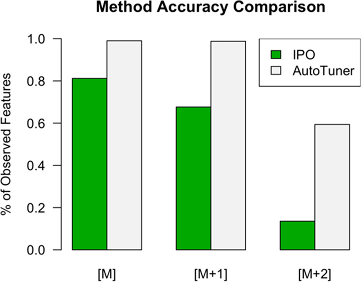
AutoTuner and IPO accuracy comparison. Percentages were determined from the number of detected standard peaks relative to the total possible set. M denotes 12Cn13C0 isotopologue; [M + 1] denotes 12Cn–113C1 isotopologue; [M + 2] denotes 12Cn–213C2 isotopologue. We normalized percentages by the total number of possible detectable peaks based on the detection of 12C standards (12Cn13C0).
Additionally, we enumerated all features matching 12Cn–113C1 and 12Cn–213C2 isotopologues of standards to determine the influence of parameter values on the detection of lower intensity features (Figure 2). We only considered these isotopologues if the 12Cn13C0 ion was present within the feature tables derived with method-specific parameters. We detected 80 out of 81 and 38 out of 64 possible 12Cn–113C1 and 12Cn–213C2 peaks, respectively, within the AutoTuner-derived feature table. We detected 46 out of 68 and 8 out of 59 possible 12Cn–113C1 and 12Cn–213C2 peaks, respectively, within the IPO-derived feature table.
We first compared the number of features from culture data generated with parameters from each algorithm to understand the influence of parameter selection on downstream data properties (Figures 3A and S5A). Each feature table contained a distinct number of total features following processing and quality control (Table S3). In positive ion mode, AutoTuner-derived parameters detected fewer unique features (203) compared to 2606 unique features detected with IPO-derived parameters (Figure 3A), while sharing 1022 features between them. A similar situation was observed in negative ion mode where AutoTuner detected 540 unique features compared to 3420 unique features found with IPO-derived parameters, while sharing 904 features (Figure S5A).
Figure 3.

Comparing the differences between positive ion mode data generated by AutoTuner and IPO on the culture dataset. (A) The overlap in the number of m/z-rt features generated by both methods. Features with an error of 5 ppm and retention time error of 20 s are placed in the intersect. (B) Comparison of the differences in structural properties for the maximum continuous wavelet transform coefficient (CWT) between peaks detected only within AutoTuner (orange) and IPO (green). Both curves are empirical cumulative distribution functions (CDF) of the calculated metric. (C) Three randomly selected EIC peaks that fall on distinct regions of the maximum CWT empirical cumulative distribution function to demonstrate how this metric influence peak shapes. The EIC shape reflects the maximal CWT rather than the parametrization method. The CDF curves were significantly different (KS-test, p < 10–4, n = 203). Results for positive mode data area CDF and negative data were similar to this data and are found in Figures S4 and S5, respectively.
We then compared the structural differences between features exclusively detected using IPO- and AutoTuner-derived parameters. We created an empirical cumulative distribution function (CDF) to compare the distribution of peak areas (Figure S5A,B) and maximum observed continuous wavelet transform (CWT) coefficients (Figures 3B and S5C) of all EIC peaks belonging to features outside of the intersect. The maximum observed CWT coefficient increases with peak steepness and may provide a measure of a peak’s chromatographic resolution (Figure 3C). The CDF of each metric was significantly different in positive (KS-Test; area: p < 10–6; CWT: p < 10–4; n = 203) and negative (KS-Test; area: p < 10–14; CWT: p < 10–8; n = 540) ionization mode data. The application of the same test on unbalanced comparisons (e.g., negative ion mode: 3420 IPO- vs 540 AutoTuner-unique features) was more highly significant than using equivalent numbers of features obtained through subsampling.
Next, we compared the abundance of features with MS/MS spectra within each unique feature table because features with MS/MS spectra can be compared to spectral databases and authenticated standards, thus enabling potential identification. In total, we observed more features with MS/MS spectra within the feature table generated with IPO-derived parameters compared to that generated with AutoTuner-derived parameters (positive: 448 vs 115; negative: 686 vs 121; both for IPO vs AutoTuner, respectively). However, this is due primarily to the greater number of features in the IPO-derived table. Indeed, relative to total features, IPO-derived features were less likely to have associated MS/MS spectra than features within the intersect of both datasets (hypergeometric test; negative ion mode: p < 10–10; positive ion mode: p < 10–10). A similar comparison revealed that MS/MS enrichment was not significantly different between AutoTuner-derived features and those within the intersect (Table S4).
Finally, using all three of the test datasets, we compared the time required to run AutoTuner and IPO (Table 3). After accounting for number of CPUs, AutoTuner ran hundreds to thousands of times faster.
Table 3. Run-Times for AutoTuner and IPO Required to Run 6 Common Samples Collected in Positive (+) and Negative (−) Ionization Modesa.
| algorithm | culture (−) | culture (+) | standards (−) | standards (+) | community (−) | community (+) |
|---|---|---|---|---|---|---|
| AutoTuner | 2 min | 9 min | 2 min | 3 min | 25 min | 26 min |
| IPO | 7 h 23 min | 28 h 40 min | 31 h 56 min | 28 h 5 min | 38 h 4 min | 21 h 27 min |
| ratio (Auto/IPO) | 1479 | 1518 | 6970 | 4238 | 715 | 396 |
| samples used | 6 | 6 | 4 | 4 | 6 | 6 |
All system time measurements were done on an 8 CPUs and 10 Gb of memory Ubuntu Xenial 16.04 Google Cloud instance. IPO ran on 8 CPUs, while AutoTuner ran on 1 CPU. The ratio accounts for the total computing power used to run both algorithms.
Testing the Robustness of the AutoTuner Estimation
Figure 4 shows the coefficient of variation and estimate values for each 11 sample subset for the parameter ppm obtained from Monte Carlo analysis on the culture and community datasets. Figures S6–S13 show the complete set of results from the Monte Carlo analysis for all parameters. For all parameter estimates, the variability of estimation decreased linearly with the number of samples used under both ionization modes (Figures 4A and S6–S13). The rendered parameter estimates were consistent with expectations based on the mass analyzer used to generate the data (Table 2). With the exception of the Maximum Peak-width parameter estimate in the community dataset and the Noise estimate in the negative culture data, all parameters had a coefficient of variation (CV) of less than or equal to 0.1 when using 9 samples to obtain the estimates (Figures S6, S8, S10, and S12).
Figure 4.
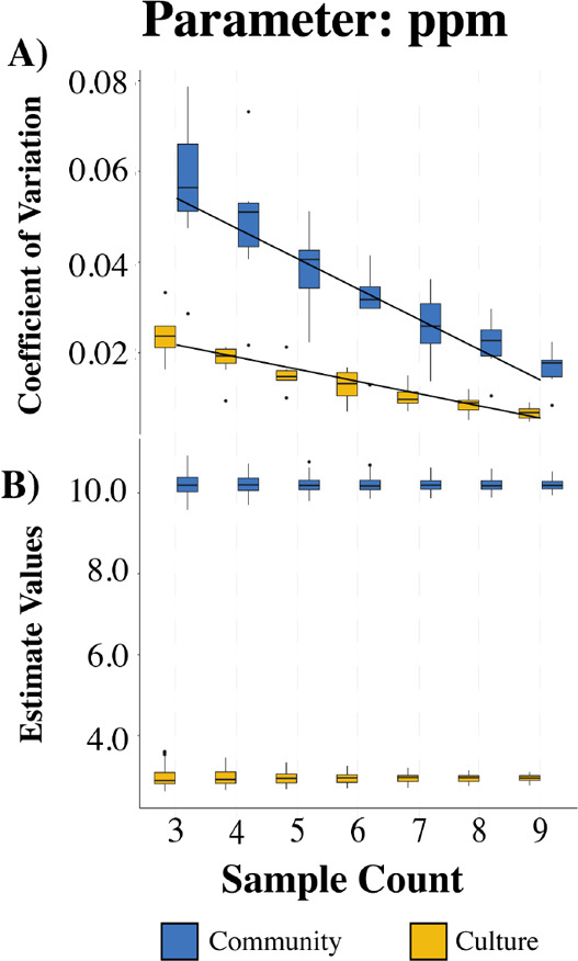
Results from the Monte Carlo experiment for parameter ppm in positive ion mode data. (A) The distribution of the coefficient of variation from parameters within the 11 sample group, while (B) shows the distribution of all estimates for ppm. Blue bars describe data collected by the qTOF instrument (community data) while yellow bars describe FT-ICR-MS data (culture data). See Figures S5–S12 for results on other parameter estimates in each ionization mode and dataset.
Discussion
AutoTuner is a robust, rapid, and high-fidelity estimator of untargeted mass spectrometry data processing parameters. Its unique design improves upon previous methods by providing a scalable framework to handle large datasets, reducing run-time, and generating high-accuracy parameters that retain known features. AutoTuner’s ease of use make it an ideal candidate to include within existing data processing pipelines.39−42 AutoTuner’s high accuracy indicates that its parameter selection is based on true data features. One possible explanation for the lower accuracy of IPO is that the peak-width of the missing standards was below the Minimum Peak-width parameter selected by IPO (Table S2 and Figure S2).
AutoTuner parameter estimates were robust across all datasets and ionization modes. Some parameters like ppm, Noise, S/N Threshold, Prefilter intensity, and Scan count reflect systematic properties inherent to the platform chromatography, mass analyzer, and/or sample matrix.43 Other parameters like Maximum peak-width are more specific to each sample; hence, the increase in the total number of samples used to estimate parameters always strengthened their robustness. The low CV values for parameter estimates suggests that using a subset of samples to generate estimates returns a set representative for all samples. On the basis of our results, we recommend the use of 9 and 12 samples to generate estimates in culture and community datasets, respectively. For most of the parameters estimated here, 9 samples proved sufficient to obtain estimates with CV values less than 0.1. The 12-parameter recommendation originated from extrapolating the linear fits of these data to obtain 0.1 CV values for remaining parameters that failed this criterion (Figures S6, S8, S10, and S12). We were unable to check the robustness of the Group difference parameter estimate, as this parameter is estimated through a nonautomatable cross sample comparison during the TIC peak detection step of the algorithm.
Although other algorithms return more parameter estimates than AutoTuner, the parameters calculated by AutoTuner represent continuous valued ones with the greatest possible number of choices. Performing a parameter sweeping optimization like previous approaches to estimate the remaining parameters after fixing the AutoTuner derived ones reduces the total combinations of available centWave parameters from a space of at least 24 × 58 possible choices of parameters to one of 40. This is because the centWave algorithm, used by both XCMS and MZmine2 data processing tools, requires tuning of 11 distinct parameters. Of these, 8 are continuously valued, meaning that they can be any real number. The remainder either are boolean values or can be one of a few discrete choices (Table S5). The reduction of the total number of combinations is achieved by optimizing 7 of the 8 continuous valued parameters. In regards to the last continuous parameter not optimized by AutoTuner, mzDiff, we performed a sensitivity analysis to show that distinct values had a minimal effect on the returned feature table (Table S6). Future contributions towards AutoTuner’s design can help the estimation of additional parameters not covered within its current design.
AutoTuner’s low run-time indicates that the algorithm is scalable (Table 3). As more and more data is generated due to increases in analytical throughput and dataset size, AutoTuner will remain a tractable option to generate estimates of metabolomics data processing parameters.4,44 Because AutoTuner estimates parameters much faster than IPO and IPO was shown to perform at a faster rate than software preceding it, we surmise that AutoTuner is the fastest parameter selection algorithm available.22
The evaluation of quality between culture dataset feature tables generated with IPO- and AutoTuner-derived parameters is impossible without performing a complete validation of all possible features. Such analyses are time-consuming, labor intensive, and beyond the scope of this manuscript. However, the measured properties of these datasets may provide some expectation for practitioners of metabolomics of how the data generated using each method may differ.
When considering the unique features identified by each algorithm in the culture dataset, AutoTuner found fewer features in each case (Figures 3 and S4). This may be due to the selection of different ppm error parameters between AutoTuner and IPO; the ppm error thresholds selected by IPO were higher under each ionization mode than those selected by AutoTuner (Table S2). AutoTuner’s lower ppm error estimates do not appear to be too stringent, as they are between 4 and 6 times greater than the instrument-recommended error threshold of 0.5 ppm and they are consistent with recommendations by the “centWave” developers.36 The size of the processed data using AutoTuner-derived parameters was in line with previous work validating the metabolome of Escherichia coli after performing stringent isotope labeling experiments and quality control filtering.26 AutoTuner feature selection does not appear to be biased toward higher intensity features, because the standard dataset processed with AutoTuner-derived parameters contained a high percentage of possible 13C isotopologues. The paucity of size-validated metabolome datasets precludes further evaluation of the feature number comparison. Within the AutoTuner-derived feature tables, those features unique to the AutoTuner-derived parameters were enriched in MS/MS relative to the unique IPO-derived features. We stress that features with MS/MS spectra cannot be assumed to be more or less important within a metabolomics dataset; however, the presence of these spectra enhances downstream identification efforts and may be desirable to some investigators.
AutoTuner has several avenues for possible improvement. First, AutoTuner could be parallelized to reduce computation time by a factor of the total number of CPUs used. Second, additional algorithms may be implemented to optimize parameters not covered here. One drawback from the speed gained in the computation through its “divide-and-conquer” approach comes at a loss of comparing EIC peaks across samples to estimate retention time correction algorithms. This challenge leaves room for the implementation of additional algorithms. Third, the replacement of the sliding window analysis with a more sophisticated and sensitive peak detection approach may eliminate the need for user input during the first portion of AutoTuner. However, this automation comes at the cost of manual inspection of the raw data. We support manual inspection of the raw data, because it provides a quality control check for the data generation steps leading up to the analysis. AutoTuner provides several built-in plotting functions to facilitate this evaluation step. Despite these minor caveats, AutoTuner is a viable and time-saving option to determine proper data processing parameters for untargeted metabolomics data.
Acknowledgments
We thank Titus Brown and Ben Temperton for advice on the algorithm validation, Arthur Eschenlauer for constructive feedback on the software design, Krista Longnecker for continuous support and discussions, Gabriel Leventhal for mathematics advice, the users of AutoTuner for debugging help through Github, and David Angeles-Albores and two anonymous reviewers for critical feedback on the manuscript. Funding support included the National GEM Consortium and NSF graduate research program fellowships (C.M.) and grants from the MIT Microbiome Center (Award 6936800, E.B.K.) and the Simons Foundation (Award ID #509034, E.B.K.).
Supporting Information Available
The Supporting Information is available free of charge at https://pubs.acs.org/doi/10.1021/acs.analchem.9b04804.
Example of AutoTuner-generated ppm error distribution, EIC peaks of standards, impact of feature intensity threshold on standard detection, positive and negative ion mode data parameter estimates and coefficients of variation, standards used to validate AutoTuner accuracy, parameters used to process data, feature count from each data set during the different stages of quality assurance processing of culture data, counts of total detected features with MS/MS, standard parameters used within the centWave algorithm, and number of unique features observed after processing data with unique mzDiff values (PDF)
The authors declare no competing financial interest.
Supplementary Material
References
- Zamboni N.; Saghatelian A.; Patti G. J. Defining the Metabolome: Size, Flux, and Regulation. Mol. Cell 2015, 58 (4), 699–706. 10.1016/j.molcel.2015.04.021. [DOI] [PMC free article] [PubMed] [Google Scholar]
- Alvarez L.; Aliashkevich A.; de Pedro M. A.; Cava F. Bacterial Secretion of D-Arginine Controls Environmental Microbial Biodiversity. ISME J. 2018, 12 (2), 438–450. 10.1038/ismej.2017.176. [DOI] [PMC free article] [PubMed] [Google Scholar]
- Kujawinski E. B.; Longnecker K.; Alexander H.; Dyhrman S. T.; Fiore C. L.; Haley S. T.; Johnson W. M. Phosphorus Availability Regulates Intracellular Nucleotides in Marine Eukaryotic Phytoplankton. Limnology and Oceanography Letters 2017, 2 (4), 119–129. 10.1002/lol2.10043. [DOI] [Google Scholar]
- White R. A.; Callister S. J.; Moore R. J.; Baker E. S.; Jansson J. K. The Past, Present and Future of Microbiome Analyses. Nat. Protoc. 2016, 11 (11), 2049–2053. 10.1038/nprot.2016.148. [DOI] [Google Scholar]
- Chong J.; Soufan O.; Li C.; Caraus I.; Li S.; Bourque G.; Wishart D. S.; Xia J. MetaboAnalyst 4.0: Towards More Transparent and Integrative Metabolomics Analysis. Nucleic Acids Res. 2018, 46 (W1), W486–W494. 10.1093/nar/gky310. [DOI] [PMC free article] [PubMed] [Google Scholar]
- Ren S.; Hinzman A. A.; Kang E. L.; Szczesniak R. D.; Lu L. J. Computational and Statistical Analysis of Metabolomics Data. Metabolomics 2015, 11, 1492–1513. 10.1007/s11306-015-0823-6. [DOI] [Google Scholar]
- Busch K. L. Chemical Noise in Mass Spectrometry. Spectroscopy 2003, 18 (3), 52–55. [Google Scholar]
- Lommen A. MetAlign: Interface-Driven, Versatile Metabolomics Tool for Hyphenated Full-Scan Mass Spectrometry Data Preprocessing. Anal. Chem. 2009, 81 (8), 3079–3086. 10.1021/ac900036d. [DOI] [PubMed] [Google Scholar]
- Jiang W.; Qiu Y.; Ni Y.; Su M.; Jia W.; Du X. An Automated Data Analysis Pipeline for GC-TOF-MS Metabonomics Studies. J. Proteome Res. 2010, 9 (11), 5974–5981. 10.1021/pr1007703. [DOI] [PubMed] [Google Scholar]
- Röst H. L.; Sachsenberg T.; Aiche S.; Bielow C.; Weisser H.; Aicheler F.; Andreotti S.; Ehrlich H.-C.; Gutenbrunner P.; Kenar E.; et al. OpenMS: A Flexible Open-Source Software Platform for Mass Spectrometry Data Analysis. Nat. Methods 2016, 13 (9), 741–748. 10.1038/nmeth.3959. [DOI] [PubMed] [Google Scholar]
- Samanipour S.; O’Brien J. W.; Reid M. J.; Thomas K. V. Self Adjusting Algorithm for the Nontargeted Feature Detection of High Resolution Mass Spectrometry Coupled with Liquid Chromatography Profile Data. Anal. Chem. 2019, 91 (16), 10800–10807. 10.1021/acs.analchem.9b02422. [DOI] [PubMed] [Google Scholar]
- Pluskal T.; Castillo S.; Villar-Briones A.; Oresic M. MZmine 2: Modular Framework for Processing, Visualizing, and Analyzing Mass Spectrometry-Based Molecular Profile Data. BMC Bioinf. 2010, 11, 395. 10.1186/1471-2105-11-395. [DOI] [PMC free article] [PubMed] [Google Scholar]
- Smith C. A.; Want E. J.; O’Maille G.; Abagyan R.; Siuzdak G. XCMS: Processing Mass Spectrometry Data for Metabolite Profiling Using Nonlinear Peak Alignment, Matching, and Identification. Anal. Chem. 2006, 78 (3), 779–787. 10.1021/ac051437y. [DOI] [PubMed] [Google Scholar]
- Myers O. D.; Sumner S. J.; Li S.; Barnes S.; Du X. One Step Forward for Reducing False Positive and False Negative Compound Identifications from Mass Spectrometry Metabolomics Data: New Algorithms for Constructing Extracted Ion Chromatograms and Detecting Chromatographic Peaks. Anal. Chem. 2017, 89 (17), 8696–8703. 10.1021/acs.analchem.7b00947. [DOI] [PubMed] [Google Scholar]
- Myers O. D.; Sumner S. J.; Li S.; Barnes S.; Du X. Detailed Investigation and Comparison of the XCMS and MZmine 2 Chromatogram Construction and Chromatographic Peak Detection Methods for Preprocessing Mass Spectrometry Metabolomics Data. Anal. Chem. 2017, 89 (17), 8689–8695. 10.1021/acs.analchem.7b01069. [DOI] [PubMed] [Google Scholar]
- Li Z.; Lu Y.; Guo Y.; Cao H.; Wang Q.; Shui W. Comprehensive Evaluation of Untargeted Metabolomics Data Processing Software in Feature Detection, Quantification and Discriminating Marker Selection. Anal. Chim. Acta 2018, 1029, 50–57. 10.1016/j.aca.2018.05.001. [DOI] [PubMed] [Google Scholar]
- Brodsky L.; Moussaieff A.; Shahaf N.; Aharoni A.; Rogachev I. Evaluation of Peak Picking Quality in LC-MS Metabolomics Data. Anal. Chem. 2010, 82 (22), 9177–9187. 10.1021/ac101216e. [DOI] [PubMed] [Google Scholar]
- Manier S. K.; Keller A.; Meyer M. R. Automated Optimization of XCMS Parameters for Improved Peak Picking of Liquid Chromatography-Mass Spectrometry Data Using the Coefficient of Variation and Parameter Sweeping for Untargeted Metabolomics. Drug Test. Anal. 2019, 11, 752. 10.1002/dta.2552. [DOI] [PubMed] [Google Scholar]
- Baran R. Untargeted Metabolomics Suffers from Incomplete Raw Data Processing. Metabolomics 2017, 13 (9), 530. 10.1007/s11306-017-1246-3. [DOI] [Google Scholar]
- Eliasson M.; Rännar S.; Madsen R.; Donten M. A.; Marsden-Edwards E.; Moritz T.; Shockcor J. P.; Johansson E.; Trygg J. Strategy for Optimizing LC-MS Data Processing in Metabolomics: A Design of Experiments Approach. Anal. Chem. 2012, 84 (15), 6869–6876. 10.1021/ac301482k. [DOI] [PubMed] [Google Scholar]
- Zheng H.; Clausen M. R.; Dalsgaard T. K.; Mortensen G.; Bertram H. C. Time-Saving Design of Experiment Protocol for Optimization of LC-MS Data Processing in Metabolomic Approaches. Anal. Chem. 2013, 85 (15), 7109–7116. 10.1021/ac4020325. [DOI] [PubMed] [Google Scholar]
- Libiseller G.; Dvorzak M.; Kleb U.; Gander E.; Eisenberg T.; Madeo F.; Neumann S.; Trausinger G.; Sinner F.; Pieber T.; et al. IPO: A Tool for Automated Optimization of XCMS Parameters. BMC Bioinf. 2015, 16, 118. 10.1186/s12859-015-0562-8. [DOI] [PMC free article] [PubMed] [Google Scholar]
- Makarov A.; Denisov E.; Kholomeev A.; Balschun W.; Lange O.; Strupat K.; Horning S. Performance Evaluation of a Hybrid Linear Ion Trap/Orbitrap Mass Spectrometer. Anal. Chem. 2006, 78, 2113–2120. 10.1021/ac0518811. [DOI] [PubMed] [Google Scholar]
- Gumustas M.; Kurbanoglu S.; Uslu B.; Ozkan S. A. UPLC versus HPLC on Drug Analysis: Advantageous, Applications and Their Validation Parameters. Chromatographia 2013, 76, 1365–1427. 10.1007/s10337-013-2477-8. [DOI] [Google Scholar]
- Mahieu N. G.; Spalding J. L.; Gelman S. J.; Patti G. J. Defining and Detecting Complex Peak Relationships in Mass Spectral Data: The Mz.unity Algorithm. Anal. Chem. 2016, 88 (18), 9037–9046. 10.1021/acs.analchem.6b01702. [DOI] [PMC free article] [PubMed] [Google Scholar]
- Mahieu N. G.; Patti G. J. Systems-Level Annotation of a Metabolomics Data Set Reduces 25 000 Features to Fewer than 1000 Unique Metabolites. Anal. Chem. 2017, 89 (19), 10397–10406. 10.1021/acs.analchem.7b02380. [DOI] [PMC free article] [PubMed] [Google Scholar]
- Domingo-Almenara X.; Montenegro-Burke J. R.; Guijas C.; Majumder E. L.-W.; Benton H. P.; Siuzdak G. Autonomous METLIN-Guided in-Source Fragment Detection Increases Annotation Confidence in Untargeted Metabolomics. Anal. Chem. 2019, 91, 3246. 10.1021/acs.analchem.8b03126. [DOI] [PMC free article] [PubMed] [Google Scholar]
- Domingo-Almenara X.; Montenegro-Burke J. R.; Benton H. P.; Siuzdak G. Annotation: A Computational Solution for Streamlining Metabolomics Analysis. Anal. Chem. 2018, 90 (1), 480–489. 10.1021/acs.analchem.7b03929. [DOI] [PMC free article] [PubMed] [Google Scholar]
- Stanstrup J.XCMS Workshop; 2017; http://stanstrup.github.io/material/presentations/1.%20XCMS.html#/.
- Hastie T.; Tibshirani R.; Friedman J.. The Elements of Statistical Learning: Data Mining, Inference, and Prediction; Springer Science & Business Media, 2013. [Google Scholar]
- Tibshirani R.; Walther G.; Hastie T. Estimating the Number of Clusters in a Data Set via the Gap Statistic. Journal of the Royal Statistical Society: Series B (Statistical Methodology). 2001, 63, 411–423. 10.1111/1467-9868.00293. [DOI] [Google Scholar]
- Johnson W. M.; Kido Soule M. C.; Kujawinski E. B. Evidence for Quorum Sensing and Differential Metabolite Production by a Marine Bacterium in Response to DMSP. ISME J. 2016, 10 (9), 2304–2316. 10.1038/ismej.2016.6. [DOI] [PMC free article] [PubMed] [Google Scholar]
- Kale N. S.; Haug K.; Conesa P.; Jayseelan K.; Moreno P.; Rocca-Serra P.; Nainala V. C.; Spicer R. A.; Williams M.; Li X.; et al. MetaboLights: An Open-Access Database Repository for Metabolomics Data. Curr. Protoc. Bioinformatics 2016, 53, 14.13.1–14.13.18. 10.1002/0471250953.bi1413s53. [DOI] [PubMed] [Google Scholar]
- Casero D.; Gill K.; Sridharan V.; Koturbash I.; Nelson G.; Hauer-Jensen M.; Boerma M.; Braun J.; Cheema A. K. Space-Type Radiation Induces Multimodal Responses in the Mouse Gut Microbiome and Metabolome. Microbiome 2017, 5 (1), 105. 10.1186/s40168-017-0325-z. [DOI] [PMC free article] [PubMed] [Google Scholar]
- Chambers M. C.; Maclean B.; Burke R.; Amodei D.; Ruderman D. L.; Neumann S.; Gatto L.; Fischer B.; Pratt B.; Egertson J.; et al. A Cross-Platform Toolkit for Mass Spectrometry and Proteomics. Nat. Biotechnol. 2012, 30 (10), 918–920. 10.1038/nbt.2377. [DOI] [PMC free article] [PubMed] [Google Scholar]
- Tautenhahn R.; Böttcher C.; Neumann S. Highly Sensitive Feature Detection for High Resolution LC/MS. BMC Bioinf. 2008, 9, 504. 10.1186/1471-2105-9-504. [DOI] [PMC free article] [PubMed] [Google Scholar]
- Kuhl C.; Tautenhahn R.; Böttcher C.; Larson T. R.; Neumann S. CAMERA: An Integrated Strategy for Compound Spectra Extraction and Annotation of Liquid Chromatography/mass Spectrometry Data Sets. Anal. Chem. 2012, 84 (1), 283–289. 10.1021/ac202450g. [DOI] [PMC free article] [PubMed] [Google Scholar]
- Broadhurst D.; Goodacre R.; Reinke S. N.; Kuligowski J.; Wilson I. D.; Lewis M. R.; Dunn W. B. Guidelines and Considerations for the Use of System Suitability and Quality Control Samples in Mass Spectrometry Assays Applied in Untargeted Clinical Metabolomic Studies. Metabolomics 2018, 14 (6), 72. 10.1007/s11306-018-1367-3. [DOI] [PMC free article] [PubMed] [Google Scholar]
- Tautenhahn R.; Patti G. J.; Rinehart D.; Siuzdak G. XCMS Online: A Web-Based Platform to Process Untargeted Metabolomic Data. Anal. Chem. 2012, 84 (11), 5035–5039. 10.1021/ac300698c. [DOI] [PMC free article] [PubMed] [Google Scholar]
- Peters K.; Bradbury J.; Bergmann S.; Capuccini M.; Cascante M.; de Atauri P.; Ebbels T. M. D.; Foguet C.; Glen R.; Gonzalez-Beltran A. PhenoMeNal: Processing and Analysis of Metabolomics Data in the Cloud. GigaScience 2019, 8, giy149. 10.1093/gigascience/giy149. [DOI] [PMC free article] [PubMed] [Google Scholar]
- Davidson R. L.; Weber R. J. M.; Liu H.; Sharma-Oates A.; Viant M. R. Galaxy-M: A Galaxy Workflow for Processing and Analyzing Direct Infusion and Liquid Chromatography Mass Spectrometry-Based Metabolomics Data. GigaScience 2016, 5, s13742-016-0115-8. 10.1186/s13742-016-0115-8. [DOI] [PMC free article] [PubMed] [Google Scholar]
- Giacomoni F.; Le Corguille G.; Monsoor M.; Landi M.; Pericard P.; Petera M.; Duperier C.; Tremblay-Franco M.; Martin J.-F.; Jacob D. Workflow4Metabolomics: A Collaborative Research Infrastructure for Computational Metabolomics. Bioinformatics 2015, 31, 1493–1495. 10.1093/bioinformatics/btu813. [DOI] [PMC free article] [PubMed] [Google Scholar]
- Han W.; Li L. Matrix Effect on Chemical Isotope Labeling and Its Implication in Metabolomic Sample Preparation for Quantitative Metabolomics. Metabolomics 2015, 11 (6), 1733–1742. 10.1007/s11306-015-0826-3. [DOI] [Google Scholar]
- Yang A.; Troup M.; Ho J. W. K. Scalability and Validation of Big Data Bioinformatics Software. Comput. Struct. Biotechnol. J. 2017, 15, 379–386. 10.1016/j.csbj.2017.07.002. [DOI] [PMC free article] [PubMed] [Google Scholar]
Associated Data
This section collects any data citations, data availability statements, or supplementary materials included in this article.