

The sasPDF method, an extension of the atomic pair distribution function (PDF) analysis to the small-angle scattering (SAS) regime, is presented. The method is applied to characterize the structure of nanoparticle assemblies with different levels of structural order.
Keywords: small-angle scattering, pair distribution function, nanoparticle assembly, self-assembly
Abstract
sasPDF, a method for characterizing the structure of nanoparticle assemblies (NPAs), is presented. The method is an extension of the atomic pair distribution function (PDF) analysis to the small-angle scattering (SAS) regime. The PDFgetS3 software package for computing the PDF from SAS data is also presented. An application of the sasPDF method to characterize structures of representative NPA samples with different levels of structural order is then demonstrated. The sasPDF method quantitatively yields information such as structure, disorder and crystallite sizes of ordered NPA samples. The method was also used to successfully model the data from a disordered NPA sample. The sasPDF method offers the possibility of more quantitative characterizations of NPA structures for a wide class of samples.
1. Introduction
With the advent of high degrees of control over nanoparticle synthesis (Murray et al., 1993 ▸; Hyeon et al., 2001 ▸; de Mello Donegá et al., 2005 ▸), attention is turning to assembling superlattices of nanoparticles (NPs) as metamaterials (Boles et al., 2016 ▸; Choi et al., 2016 ▸), and applications of nanoparticle assembly (NPA)-based devices such as solar cells and field effect transistors have been demonstrated (Talapin & Murray, 2005 ▸; Sargent, 2008 ▸; Talapin et al., 2010 ▸). It is crucial to study the structures of these NPAs if their properties are to be optimized. For example, it has been shown that the mechanical (Akcora et al., 2009 ▸), optical (Young et al., 2014 ▸), electrical (Vanmaekelbergh & Liljeroth, 2005 ▸) and magnetic (Sun et al., 2000 ▸) properties can be further engineered by controlling the spatial arrangement of the constituents in the NPA.
Getting detailed quantitative structural information from NPAs, especially in three dimensions, is a challenging and largely unsolved problem. Small-angle scattering (SAS) and electron microscopy have been the major techniques for studying the structure of NPAs (Murray et al., 2000 ▸; Talapin et al., 2009 ▸). The technique of transmission electron microscopy (TEM) yields high-resolution images of NPAs. To obtain quantitative structural information it is necessary to either analyze the images manually (Wang, 2000 ▸) or match observed images with patterns that are algorithmically generated from known structures (Shevchenko et al., 2006 ▸). This approach can yield the structure types (Zhuang et al., 2008 ▸) but does not typically result in the kind of quantitative 3D structural information we are used to obtaining for atomic structures of crystals, including accurate inter-particle vectors and distributions of inter-particle distances, or the range of structural coherence of the packing order. It is desirable to explore scattering approaches that can yield that kind of information.
The technique of small-angle X-ray or neutron scattering has been an important tool to study objects that have sizes from nano- to micrometre length scales (Turkevich & Hubbell, 1951 ▸; Glatter, 1977 ▸; Guinier, 1994 ▸; Koch et al., 2003 ▸), such as large nanocrystals (Polte et al., 2010 ▸) and biological molecules (Koch et al., 2003 ▸), yielding information about the intrinsic shape, size distributions and scattering density of objects on these scales (Glatter, 1977 ▸; Beaucage, 1995 ▸; Pedersen, 1997 ▸; Volkov & Svergun, 2003 ▸; Beaucage et al., 2004 ▸).
When these nanoscale objects aggregate, correlation peaks appear in the SAS data, resembling atomic scale interference peaks (diffuse scattering and Bragg peaks) but encoding information about particle packing rather than atomic packing (Murray et al., 2000 ▸; Nykypanchuk et al., 2008 ▸). Obtaining structural information about the NPAs from these correlation peaks appears to be a promising approach. Although the recent developments in SAS modeling demonstrate the ability to account for phase, morphology and orientations of NPs in a lattice (Yager et al., 2014 ▸; Lu et al., 2019 ▸), fitting the SAS data with robust structural models to obtain quantitative information about the structure has barely been explored (Macfarlane et al., 2011 ▸).
On the other hand, the atomic pair distribution function (PDF) analysis of X-ray and neutron powder diffraction has proven to be a powerful tool for characterizing local order in materials and for extracting quantitative structural information (Proffen et al., 2005 ▸; Egami & Billinge, 2012 ▸; Zobel et al., 2015 ▸; Keen & Goodwin, 2015 ▸) when the atoms are not long-range ordered, as is the case in nanoparticles. Here we extend PDF analysis to handle correlation peaks in small-angle scattering data, allowing us to study the arrangement of particles in nanoparticle assemblies using the same quantitative modeling tools that are available for studying the atomic arrangements in nanoparticles themselves. We describe the extension of the PDF equations in the SAS regime and the data collection protocol for optimum data quality. We also present the PDFgetS3 software package, which can be readily used to extract the PDF from small-angle scattering data. We then apply our method, ‘sasPDF’, to investigate structures of some representative NPA samples with different levels of structural order.
2. Samples
To test the method we obtained SAS data from the samples listed in Table 1 ▸. Synthesis details of these NPA samples can be found in the references listed in the table.
Table 1. Nanoparticle assemblies considered in this study.
Building block indicates the NP and surfactant linkers used to build the assemblies. D is the particle diameter (one standard deviation in parentheses) estimated from TEM images and reported in the original publications listed in the Reference column. Beamline is the X-ray beamline where the SAS data were measured (see text for details). PMA is poly(methyl acrylate) and DDT is dodecanethiol.
3. sasPDF method
The data were collected using a standard small-angle X-ray scattering setup at an X-ray synchrotron source, with a 2D area detector mounted perpendicular to the beam in transmission geometry. Both the Cu2S NPA and the SiO2 NPA samples were measured at beamline 11-BM at the National Synchrotron Light Source II (NSLS-II). The Cu2S NPA powders were sealed between two rectangular Kapton tapes with a circular deposited area of diameter about 3 mm and thickness about 0.2 mm. The SiO2 NPA formed a circular free-standing stable film of diameter about 5 mm and thickness about 1 mm which was mounted perpendicular to the beam and no further sealing was carried out. The scattering data of the Cu2S NPA and SiO2 NPA samples were collected with a Pilatus 2M (Dectris, Switzerland) detector with a sample–detector distance of 2.02 m using an X-ray wavelength of 0.918 Å. An example of a diffraction image from the Cu2S NPA is shown in the inset of Fig. 1 ▸.
Figure 1.

Example of the 1D diffraction pattern  from the Cu2S NPA sample. The data were collected with the spot exposure time and scan exposure time reported in the text. The inset shows the corresponding 2D diffraction image. The horizontal stripes in the image are from the dead zone between panels of the detector. The diagonal line is the beam-stop holder.
The scattering from these samples is isotropic as the sample consists of powders of randomly oriented NPA crystallites, and the 2D diffraction images can be reduced to a 1D diffraction pattern, , by performing an azimuthal integration around rings of constant scattering angle on the detector. This was done using pyFAI (Ashiotis et al., 2015 ▸) and requires the calibration of the experiment geometry described below. The integrated 1D pattern from the 2D diffraction image is shown in Fig. 1 ▸. The relative positions and intensities of sharp peaks in originate from the Debye–Scherrer rings in the 2D image.
We need to use a data acquisition strategy that mitigates the effects of X-ray beam damage to the sample. The linkers that connect nanoparticles in the assemblies play a crucial role for the NPA structure formed but are susceptible to degradation in the intense X-ray beam, which may result in changes in the NPA structure. To describe the strategy we separate the concepts of the ‘spot exposure time’ and the ‘scan exposure time’. The latter is the total integrated exposure time required to obtain a data set with sufficient statistics. The former is the length of time that any spot on the sample is exposed. The scan exposure then consists of multiple spot exposures, where the sample is translated after each spot exposure so that a fresh region of sample is exposed. For ease of experimentation we seek a spot exposure time that is as long as possible whilst ensuring that the sample has not degraded significantly during that exposure. We have found that the maximum safe spot exposure time depends on the nature of the NPA sample, as well as experimental conditions such as X-ray energy, flux and sample temperature. Determining it therefore requires a trial-and-error approach. To choose the optimal spot exposure time we locate the beam on a fixed spot of the sample and take a sequence of short exposures, monitoring for significant changes in the intensity of the strongest correlation peak in . The spot exposure time determined in this way for our experimental setup was 30 s for both Cu S NPA and SiO NPA samples, and the scan exposure time was 5 min (30 s, 10 spots) for the Cu2S NPA sample and 10 min (30 s, 20 spots) for the SiO NPA sample.
The scan exposure time is estimated via an assessment of noise in the PDF given a desired  , but it depends sensitively on the counting statistics in the high-Q region of the diffraction pattern, which are easiest to assess by looking in the high-Q region of the reduced structure function
  . For illustration purposes, the effect of scan exposure time on (and the resulting PDF) is illustrated in Fig. 2 ▸.
Figure 2.
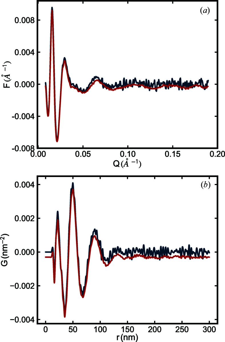
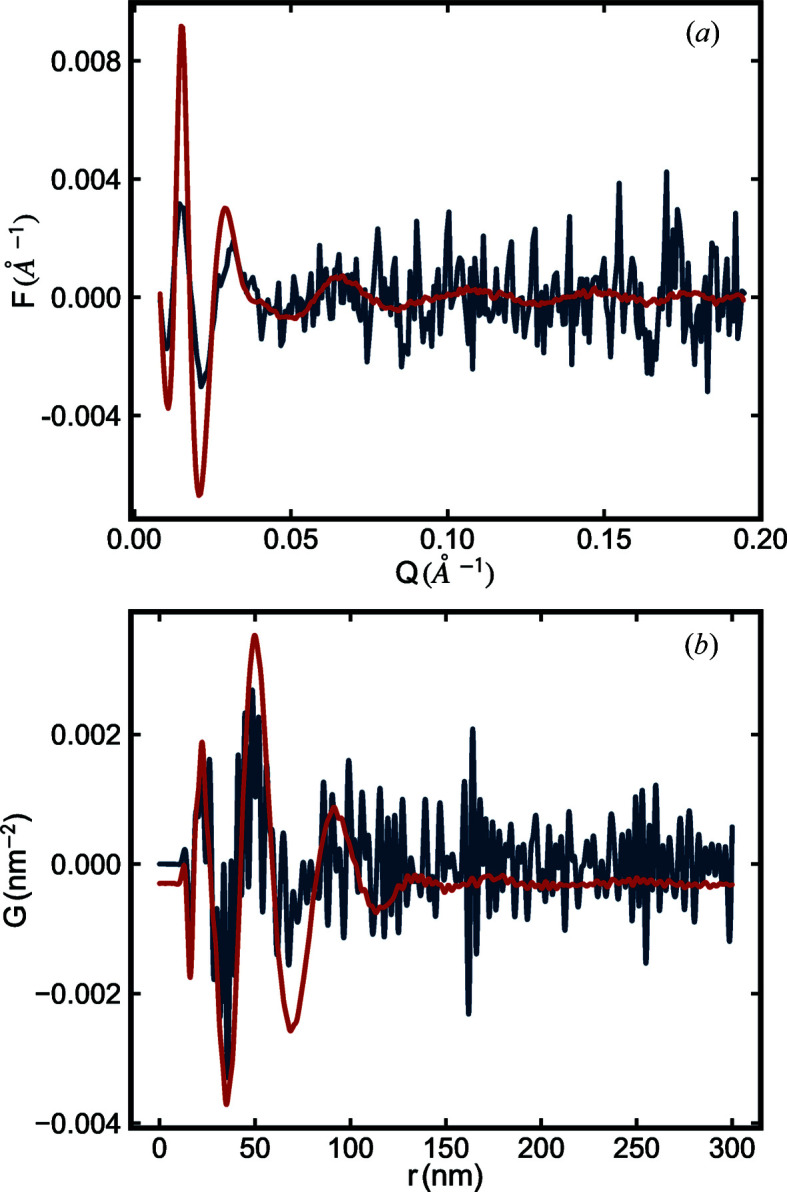
(a) Reduced structure functions and (b) PDFs  of the SiO2 NPA sample with different scan exposure times. The blue line is from data with 1 s scan exposure time and the red line is from data with 30 s scan exposure time. In both panels, data are plotted with a small offset for ease of viewing. In both cases, the form factor was measured with a scan exposure time of 600 s.
For the calibration of the experimental geometry, such as sample–detector distance and detector tilting, we use the calibration capability in the Python package pyFAI (Ashiotis et al., 2015 ▸). We first measured silver behenate (AgBh) (Gilles et al., 1998 ▸) as a well characterized calibration sample. The d spacing of the calibration sample, the X-ray wavelength and the pixel dimensions of the detector are known, which allows the geometric parameters to be refined in pyFAI. We found that selecting the strongest few rings (even just two or three work well) in the image allowed a stable refinement of the calibration parameters.
Finally, in this study we also consider legacy data from measurements carried out previously (Nykypanchuk et al., 2008 ▸). The data of the Au NPA sample were collected at beamline X21 at the National Synchrotron Light Source from a sample loaded into a wax-sealed 1 mm diameter quartz capillary. The scattering data were collected with a MarCCD (Rayonix, USA) area detector using an X-ray wavelength of 1.55 Å. Details of the measurements are reported by Nykypanchuk et al. (2008 ▸).
The PDF, denoted , is a truncated sine Fourier transform of the reduced structure function  (Egami & Billinge, 2012 ▸) :
Since can be easily computed once  is available, we will first focus on the precise definition of and its relation to the measured diffraction pattern . The measured intensity depends on experimental details such as the flux and beam size of the X-ray source, the data collection time, and the sample density. From the point of view of developing the sasPDF formalism, we will focus on the coherent scattering intensity
  (Egami & Billinge, 2012 ▸), which is obtained after correcting for the experimental factors as we describe below.
The coherent scattering intensity from a unit cell with  atoms is (Egami & Billinge, 2012 ▸; Guinier, 1963 ▸)
where  is the scattering vector, and
  and
and  are the atomic form factor amplitude and position of the mth atom in the unit cell, respectively.
If the scattering from a sample is isotropic, for example, it is an untextured powder or a liquid with no anisotropy, the observed scattering intensity will depend only on the magnitude of ,  , and not its direction in space. The observed scattering intensity in this case will depend on the orientationally averaged
  ,
,
where  denotes the orientational average.
This formalism is readily extended to the case where the scattering objects are not atoms but are some other finite-sized object, for example nanoparticles. In this case, the atomic form factor would be replaced with the form factor for the scattering objects in question. The form factor  for a generalized scatterer, with volume V and electron density as a function of position
  , is (Guinier, 1963 ▸)
where  is the average electron density of the ambient environment of the scatterers.
In situations where there is only one type of scatterer we pull the form factors out of the sum (Egami & Billinge, 2012 ▸). Furthermore, if the form factors and the structure factors are separable, equation (3) may be further simplified to
This is valid for spherical or nearly spherically shaped particles and may be more broadly true (Guinier et al., 1955 ▸; Kotlarchyk & Chen, 1983 ▸; Li et al., 2016 ▸), though if the shape of the particle results in an orientation that depends on the packing, for example a long axis lies along a particular crystallographic direction in the nanoparticle assembly, this approximation will not be ideal and equation (3) would have to be used. We have not tested how badly the approximation breaks down in these circumstances.
Following the Faber–Ziman formalism (Faber & Ziman, 1965 ▸)
we substitute 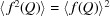 and equation (6) becomes
This expression is equivalent to representing the scatterers as points at the position of their scattering center, convoluted with their electron distributions. The resulting structure function, , yields the arrangement of scatterers in the sample. This expression is often expressed in the SAS literature as (Guinier, 1963 ▸)
where  is equivalent to
  (Guinier, 1963 ▸), the orientational average of the square of the form factor. We note that, as with the atomic PDF, the above analysis can be generalized to the cases of scattering from multiple types of scatterers (Kotlarchyk & Chen, 1983 ▸; Yager et al., 2014 ▸; Senesi & Lee, 2015 ▸), and in the SAS case approximate corrections for asphericity of the electron density (Jones et al., 2010 ▸; Ross et al., 2015 ▸; Zhang et al., 2015 ▸) may be applied.
To determine we need to have . can be computed from a given electron density or measured directly. For the case of an NPA sample, the precise scattering properties of the nanoparticle ensemble in the sample, including any polydispersity or distribution of geometric shapes, are not always known. Therefore, it is best to measure the form factor directly, as described below. In general, we do not know or all of the experimental factors (for example, the incident flux, multiple scattering and so on). The algorithm (Billinge & Farrow, 2013 ▸) that is widely used for carrying out corrections for these effects in the atomic PDF literature (Juhás et al., 2013 ▸) is also suitable for SAS data. It takes advantage of our knowledge of the asymptotic behavior of the function to obtain an ad hoc but robust estimation of from the measured . This is described in detail by Juhás et al. (2013 ▸). The resulting scale of the PDF is not well determined, but when fitting models to the data this is not a problem (Peterson et al., 2003 ▸), and in practice it gives close to a correct scale for high-quality measurements. Here we show that we can take the same approach to obtain the PDF from the measured SAS data.
In the test experiments we describe here, in each case the form factor of the nanoparticles was obtained from a measurement. The NPs are suspended in solvent at a sufficient dilution to avoid significant inter-particle correlations. If the NPs start aggregating in the solution, as a primary signature, a bump appears in the scattering intensity, at the Q value corresponding to the nearest-neighbor distance, and observation of such a bump may indicate a problem with the form factor sample. However, if we suspect aggregation or other modifications, like dimerization, occured to the sample, a more sophisticated, model-independent analysis on the scattering intensity is preferred (Kamysbayev et al., 2019 ▸; Lan et al., 2020 ▸) for identifying these changes and determining the validity of the measured form factor signal. The SAS signal of the dilute NP solution is measured with good statistics over the same range of Q as the measurement of the nanoparticle assemblies themselves, and ideally on the same instrument. The signal of the solvent and its holder is also measured and then subtracted from the SAS signal of the dilute NP solution to obtain the correct particle form factor signal. We emphasize that it is important to measure exactly the same batch of NPs to have an accurate form factor for the NPA sample considered.
A form factor measured with high statistics is crucial as the signal in is weak in the high-Q region and noise from the measurement can be significant in this region. Fig. 3 ▸ shows the effect on (and the resulting PDF) when processed using from different scan exposure times. It is clear that the statistics of the form factor measurement have a significant effect on the results. In cases where the signal in does not change rapidly it may be smoothed to reduce the effects of limited statistics, at the cost of possibly introducing bias if the smoothing is not done ideally. This will be particularly relevant when the nanoparticles are not monodisperse, as is somewhat common.
Figure 3.
(a) Reduced structure functions and (b) PDFs of the SiO2 NPA sample processed with form factor from different scan exposure times. The blue line corresponds to a form factor measured for 30 s and the red line to a form factor collected for 600 s. In both cases, the scan exposure time for the NPA sample was 600 s. In both panels, data are plotted with a small offset for ease of viewing.
The experimental PDF is then obtained via the Fourier transformation, equation (1). The success of the sasPDF method depends heavily on having good statistics (high signal-to-noise ratio) throughout the entire diffraction pattern and the form factor , as important information about the structure may reside in the high-Q region where the signal intensity is weak. It is recommended to use intense radiation sources such as synchrotrons. A comparison in data quality from an in-house instrument and a synchrotron source is shown in Fig. 4 ▸.
Figure 4.
(a) Reduced structure functions and (b) PDFs of the SiO2 NPA sample. The blue line is from data collected at Columbia University using a SAXSLAB (Amherst, MA) instrument with a 2 h (7200 s) scan exposure time for both  and measurements. The red line is from data collected at beamline 11-BM, NSLS-II, with 30 s scan exposure time for both and measurements.
4. Software
To facilitate the sasPDF method, we implemented the PDFgetS3 software program for extracting the sasPDF from experimental data. Information about obtaining the software is provided on the DiffPy web site (https://www.diffpy.org). The software is currently supported in Python 2 (2.7) and Python 3 (3.4 and above). It requires a license and is free for researchers conducting open academic research, but other uses require a paid license.
The PDFgetS3 program takes in a measured diffraction pattern and a form factor as the inputs, applies a series of operations such as subtraction of experimental effects and form factor normalization, and outputs the PDF . If the square of the orientationally averaged form factor  is available, both and can be specified in the program, and will be computed from equation (6), which accounts for the anisotropy of scatterers in the material. Processing parameters used in PDFgetS3 operations, such as the form factor file, the Q range of the Fourier transformation on and the r-grid of the output , can be set in a configuration file as detailed by Juhás et al. (2013 ▸). Similarly to PDFgetX3, an interactive window for tuning these processing parameters is also available in PDFgetS3. An illustration of this interactive interface is shown in Fig. 5 ▸.
Figure 5.

Illustration of the interactive interface for tuning the process parameters in the PDFgetS3 program.
Sliders for each processing parameter allow the user to inspect the effect on the output PDF data immediately.
Once the optimal processing parameters are determined on the basis of the quality of the PDF, those parameter values will be stored as part of the metadata in the output file. The final values of  and
and  should be used when calculating the PDF from a structure model, as these parameters contribute to the ripples in the PDF (Peterson et al., 2003 ▸). Full details on how to use the program are available on the DiffPy web site.
5. PDF method
The PDF gives the scaled probability of finding two scatterers in a material a distance r apart (Egami & Billinge, 2012 ▸). For a macroscopic object with N scatterers, the atomic pair density,  , and can be calculated from a known structure model using
and
Here,  is the number density of scatters in the object.
  is the orientationally averaged form factor of the mth scatterer.
  denotes the sample average of
  over all scatterers in the material, where
  is the number of scatterers that are of the same kind as the mth scatter. Finally,
  is the distance between the mth and nth scatterers. We use equation (10) to fit the PDF generated from a structure model to a PDF determined from experiment.
PDF modeling, where it is carried out, is performed by adjusting parameters of the structure model, such as the lattice constants, positions of scatterers and particle displacement parameters (PDPs), to maximize the agreement between the theoretical and an experimental PDF. In practice, the delta functions in equation (10) are Gaussian-broadened to account for thermal motion of the scatterers and the equation is modified with a damping factor to account for instrument resolution effects. The modeling of sasPDF can be done seamlessly with tools developed in the atomic PDF field, with parameter values scaled accordingly. We outline the modeling procedure using PDFgui (Farrow et al., 2007 ▸), which is widely used to model the atomic PDF. In PDFgui, the nanoparticle arrangements can simply be treated analogously to atomic structures, with a unit cell and fractional coordinates, but the lattice constants reflect the size of the NPA, usually ranging from 10 nm = 100 Å to 100 nm = 1000 Å. The atomic displacement parameters defined in PDFgui can be directly mapped to the particle displacement parameters in the sasPDF case and, empirically, we find the PDP values are roughly four to five orders of magnitude larger than the values of their counterparts on the atomic scale. Therefore, starting values of 500 Å are reasonable. These will be adjusted to the best-fit values during the refinement.
The PDF peak intensity depends on the scattering length of the relevant particle, which in the case of X-rays scattering off atoms is the atomic number of the atom. For the sasPDF case we do not know explicitly how to scale the scattering strength of the particles, but for systems with a single scatterer, this constitutes an arbitrary scale factor that we neglect.
The measured sasPDF signal falls off with increasing r. The damping may originate from various factors, for example, the instrumental Q-space resolution (Egami & Billinge, 2012 ▸) and finite range of order in the superlattice assembly. In PDFgui there is a Gaussian damping function  ,
,
We define the parameter  ,
,
which is the distance where about one-third of the sasPDF signal disappears completely. It is also possible to generalize the modeling process to the case of a customized damping function and non-crystallographic structure with Diffpy-CMI (Juhás et al., 2015 ▸), which is a highly flexible PDF modeling program. In the following section, we use PDFgui for modeling data from more ordered samples (Au NPA and CuS NPA) and Diffpy-CMI for modeling data from a disordered sample (SiO2 NPA).
6. Application to representative structures
To illustrate the sasPDF method we have applied it to some representative nanoparticle assemblies from the literature (Nykypanchuk et al., 2008 ▸; Han et al., 2008 ▸; Bilchak et al., 2017 ▸). The first example is from DNA-templated gold nanoparticle superlattices, originally reported by Nykypanchuk et al. (2008 ▸). The measured intensity, , the reduced total structure function, , and the PDF, , are shown in Figs. 6 ▸(a), 6 ▸(b) and 6 ▸(c), respectively.
Figure 6.
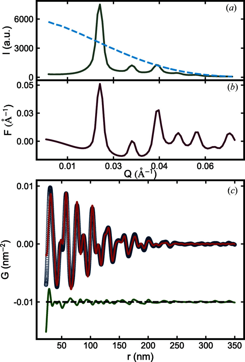
Measured (a) scattering intensity (gray) and form factor (dashed blue), (b) reduced total structure function (red), and (c) PDF (open circle) of the Au NPA. In (c), the PDF calculated from the b.c.c. model is shown in red and the difference between the measured PDF and the b.c.c. model is plotted in green with an offset.
It is clear that the data corrections and normalizations to get result in a more prominent signal in the high-Q regime of the scattering data and a highly structured PDF after the Fourier transform [Fig. 6 ▸(c)].
The PDF signal dies off at around 350 nm, which puts a lower bound on the size of the NPA. The first peak in the PDF is located at 30.07 nm, which corresponds to the nearest inter-particle distance in the assembly. This distance is expected because the shortest inter-particle distance can be approximated as the average size of Au NPs (11.4 nm) plus the average surface-to-surface distance ( ) between nearest-neighbor NPs (18 nm) (Nykypanchuk et al., 2008 ▸). Peaks beyond the nearest neighbor give an indication of characteristic inter-particle distances in the assembly and codify the 3D arrangement of the nanoparticles in space.
A semi-quantitative interpretation of conventional powder diffraction data suggested the Au NPA forms a body-centered cubic (b.c.c.) structure (Nykypanchuk et al., 2008 ▸). We therefore test the b.c.c. model against the measured PDF. The fit is shown in Fig. 6 ▸(c) and the refined parameters are reproduced in Table 2 ▸.
Table 2. Refined parameters for NPA samples.
The Model row specifies the structural model used to fit the measured PDF. a is the lattice constant of the unit cell. PDP stands for particle displacement parameter, which is an indication of the uncertainty in position of the nanoparticles. is the standard deviation of the Gaussian damping function defined in equation (12). Scale is a constant factor multiplying the calculated PDF.  is the residual function, commonly used as a measure for the goodness of fit
| Au NPA | CuS NPA |
|
|---|---|---|
| Model | B.c.c. | F.c.c. |
| a (nm) | 34.73 | 26.55 |
| PDP (nm2) | 4.78 | 0.253 |
|
(nm) |
83.3 | 61.4 |
| Scale | 0.537 | 0.361 |
|
|
0.172 | 0.221 |
The agreement between the b.c.c. model and the measured data is good. We refine a lattice parameter that is ∼3% smaller than the value reported from the semi-quantitative analysis. Additionally, the PDF gives information about the disorder in the system in the form of the crystallite size (∼350 nm) and the PDP, the nanoparticle assembly version of the atomic displacement parameter in atomic systems. The PDF-derived crystallite size is drastically smaller than the value (∼ 500 nm) estimated from the FWHM of the first correlation peak (Nykypanchuk et al., 2008 ▸), and it is clear by visual inspection of the PDF that the ∼ 500 nm value is an overestimate. These results suggest that even in the case where it is straightforward to infer the geometry of the underlying assembly using qualitative and semi-quantitative means there is an advantage to carrying out a more quantitative sasPDF analysis.
Next we consider the data set from the DDT-capped Cu2S NPA (Han et al., 2008 ▸). In this case the form factor was measured on an in-house Cu Kα instrument. This was necessary in the current case because the instability of the nanoparticles in suspension prevented a good measurement being made at the synchrotron. As a result, the form factor measurement was somewhat noisy [Fig. 7 ▸(a), blue curve], and we elected to smooth it by applying a Savitzky–Golay filter (Orfanidis, 1996 ▸). The smoothing parameters of window size and polynomial order were selected as 13 and 2, respectively, on the basis of a trial-and-error approach optimized to result in a good smoothing without changing the shape of the signal. The smoothed curve is shown in Fig. 7 ▸(a) (red curve). It is worth noting that, in general, a smoothing process may start failing when the signal-to-noise ratio in the data is below a certain threshold, and so good starting data are always desirable. A conventional semi-quantitative analysis on diffraction data from the sample collected on an in-house Cu Kα instrument is shown in Fig. 8 ▸. It suggests the NPA forms a face-centered cubic (f.c.c.) structure with an inter-particle distance of 18.8 nm. The SAS PDF obtained from the same NPA sample is shown in Fig. 9 ▸. It clearly shows that the peaks die out at around 300 nm, which again signifies the crystallite size of the assembly. The first peak of the measured PDF is at 18.5 nm, corresponding to the inter-particle distance in the NPA. This value is about 1.6% smaller than the value estimated from the semi-quantitative analysis.
Figure 7.

(a) Form factor signal from Cu2S NPs. The blue line represents the raw data collected at an in-house instrument and the red line the data smoothed by applying a Savitzky–Golay filter with window size 13 and fitted polymer order 2. (b) Reduced structure functions, , and (c) PDFs, , from the Cu2S NPA sample. In both panels, blue represents the data processed with the raw form factor signal and red represents the data processed with a smoothed form factor signal. Curves are offset from each other slightly for ease of viewing.
Figure 8.

Semi-quantitative structural analysis on the Cu2S NPA sample.
Figure 9.

Measured PDF (open circles) of a Cu2S NPA sample with the best-fit PDF from the f.c.c. model (red line). The difference curve between the data and model is plotted with an offset in green. The inset shows the region of the first four nearest-neighbor peaks of the PDF along with the best-fit f.c.c. model.
The best-fit PDF of a close-packed f.c.c. structural model is shown in red in the figure, and refined structural parameters are presented in Table 2 ▸.
The f.c.c. model yields a rather good agreement with the measured PDF of the Cu2S NPA in the short-range region (up to ∼130 nm). Interestingly, the refined lattice parameter of this cubic model is 26.55 nm, from which we can calculate an average inter-particle spacing of 18.78 nm, which is much closer to the value estimated from the in-house data than the value obtained by directly extracting the position of the first peak in the PDF. The first peak in the PDF calculated from the model lines up with that from the data at 18.5 nm, which means that the position of the peak, as extracted from the peak maximum, underestimates the actual inter-particle distance by ∼1.5%. This may be due to the sloping background in the function (Egami & Billinge, 2012 ▸). Quantitative modeling is always preferred for obtaining the most precise determination of inter-particle distance.
The region of the first four nearest-neighbor peaks in the PDF, together with the fit, is shown in the inset to Fig. 9 ▸. A close investigation of this region shows subtle shifts in peak positions between the measured PDF and the refined f.c.c. model. At around 26 nm (second peak), the peak from the refined model is shifted to higher r compared with the measured data, while at around 33 nm (third peak), the relative shift in peak position is towards the low-r direction. These discrepancies suggest the NPA structure is more complicated than a simple f.c.c. structure and may reflect the presence of internal twined defects (e.g. Banerjee et al., 2020 ▸). Furthermore, it is clear that signal persists in the measured PDF in the high-r region that is not captured by the single-phase damped f.c.c. model. There is clearly more to learn about the structure of the NPA by finding improved structural models and fitting them to the PDF, though this is beyond the scope of the current paper.
The refined PDP value of the DDT-capped Cu2S NPA is significantly smaller than that of the DNA-templated Au NPA described above. A small PDP means the positional disorder of the NPs is small, which would be expected with shorter, more rigid, linkers between the particles. The inter-particle distance (18.8 nm) can be decomposed into the sum of the average particle diameter (16.1 nm) and the particle-surface to particle-surface distance,  nm. According to the chemistry, the linker would have length 1.7 nm in the fully stretched out state, which would result in a maximal
  nm if the linkers were stretched out and oriented radially. Half the observed surface–surface distance is
  nm. This result is reasonable, suggesting the linkers are either not straight or not radial, or possibly partially interleaved. Nonetheless, this shorter linker would be expected to be more rigid and therefore consistent with our observation of a smaller PDP value from the sasPDF analysis.
Finally, we consider a data set from a more disordered system, the PMA-capped SiO2 NPA sample. The molecular weight and density of the capping polymers can be varied and in the current sample were 0.47 chains nm−2 and 132 kDa, respectively. Studies had suggested that similar NPA samples exhibit no structural order, on the basis of an empirical metric using the height of the first peak in the measured (Bilchak et al., 2017 ▸). Here we apply the sasPDF method to obtain a more complete understanding of the structure of this NPA.
To start we want to verify whether there is any evidence for close packing of the NPs, so we start with f.c.c., hexagonal close-packed (h.c.p.) and icosahedral models (Baus, 1983 ▸) to see if any good agreement between the structural model and the data can be achieved. The results are shown in Fig. 10 ▸.
Figure 10.
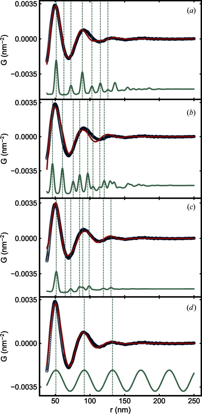
Measured PDF (open circles) of the SiO2 NPA sample and calculated PDFs (solid lines) from (a) f.c.c., (b) h.c.p., (c) icosahedral and (d) damped sine wave models. In each panel, the line in red is the PDF calculated from the corresponding model with optimum parameters. From (a) to (c), the line in gray is the PDF calculated from the same model but with small PDPs. In (d), the line in gray is the PDF calculated from the undamped sine wave model. Dashed lines indicate maxima of the sharper PDFs in each panel.
A highly broadened version of the f.c.c. model yields a reasonable agreement with the data [Fig. 10 ▸(a)]. The PDF of the f.c.c. structure is shown in gray in the figure, and after significant broadening it yields the red curve. Other close-packed cluster models, h.c.p. and icosahedral, were also tried [Figs. 10 ▸(b) and 10 ▸(c)]. Finally, a damped sine wave model that is appropriate for highly disordered systems where on average the packing around a central atom is completely isotropic was tried [Fig. 10 ▸(d)] (Cargill, 1975 ▸; Konnert & Karle, 1973 ▸; Doan-Nguyen et al., 2014 ▸). The f.c.c. and h.c.p. structures would be expected for close-packed hard spheres. Interestingly, in the current case, the very simple damped sine wave model with only three parameters yields a more satisfactory fit to the data than the more complicated (with 4–5 parameters) close-packed models, suggesting that we have soft-sphere-like packing in the current case. This finding will be explored in more detail in another publication (Liu et al., 2020 ▸). This example shows how inter-particle packing may be examined using the sasPDF method even when there is no long- or intermediate-range order.
7. Conclusions
A comprehensive understanding of the structure is needed to understand nanoparticle assemblies and design new ones with directed properties. The sasPDF method provides a new quantitative way for investigating the structures of NPAs. We describe this approach and show its advantages for obtaining a more complete understanding on the structure of NPAs.
Funding Statement
This work was funded by U.S. Department of Energy, Office of Basic Energy Sciences grants SC-0008772, SC-0019375, and DE-AC02-98CH10886. National Science Foundation, Directorate for Engineering grants CBET-1629502 and CHE-1905290. U.S. Department of Energy grant DE- SC0012704. to Pavol Juhas. U.S. Department of Energy, Office of Science grant DE-SC0012704.
References
- Akcora, P., Liu, H., Kumar, S. K., Moll, J., Li, Y., Benicewicz, B. C., Schadler, L. S., Acehan, D., Panagiotopoulos, A. Z., Pryamitsyn, V., Ganesan, V., Ilavsky, J., Thiyagarajan, P., Colby, R. H. & Douglas, J. F. (2009). Nat. Mater. 8, 354–359. [DOI] [PubMed]
- Ashiotis, G., Deschildre, A., Nawaz, Z., Wright, J. P., Karkoulis, D., Picca, F. E. & Kieffer, J. (2015). J. Appl. Cryst. 48, 510–519. [DOI] [PMC free article] [PubMed]
- Banerjee, S., Liu, C.-H., Jensen, K. M. Ø., Juhás, P., Lee, J. D., Tofanelli, M., Ackerson, C. J., Murray, C. B. & Billinge, S. J. L. (2020). Acta Cryst. A76, 24–31. [DOI] [PMC free article] [PubMed]
- Baus, M. (1983). Mol. Phys. 50, 543–565.
- Beaucage, G. (1995). J. Appl. Cryst. 28, 717–728.
- Beaucage, G., Kammler, H. K. & Pratsinis, S. E. (2004). J. Appl. Cryst. 37, 523–535.
- Bilchak, C. R., Buenning, E., Asai, M., Zhang, K., Durning, C. J., Kumar, S. K., Huang, Y., Benicewicz, B. C., Gidley, D. W., Cheng, S., Sokolov, A. P., Minelli, M. & Doghieri, F. (2017). Macromolecules, 50, 7111–7120.
- Billinge, S. J. L. & Farrow, C. L. (2013). J. Phys. Condens. Mater. 25, 454202. [DOI] [PubMed]
- Boles, M. A., Engel, M. & Talapin, D. V. (2016). Chem. Rev. 116, 11220–11289. [DOI] [PubMed]
- Cargill, G. S. (1975). Solid State Phys. 30, 227–320.
- Choi, J.-H., Wang, H., Oh, S. J., Paik, T., Sung, P., Sung, J., Ye, X., Zhao, T., Diroll, B. T., Murray, C. B. & Kagan, C. R. (2016). Science, 352, 205–208. [DOI] [PubMed]
- Doan-Nguyen, V. V. T., Kimber, S. A. J., Pontoni, D., Reifsnyder Hickey, D., Diroll, B. T., Yang, X., Miglierini, M., Murray, C. B. & Billinge, S. J. L. (2014). ACS Nano, 8, 6163–6170. [DOI] [PubMed]
- Egami, T. & Billinge, S. J. L. (2012). Underneath the Bragg Peaks: Structural Analysis of Complex Materials. 2nd ed. Amsterdam: Elsevier.
- Faber, T. E. & Ziman, J. M. (1965). Philos. Mag. 11, 153–173.
- Farrow, C. L., Juhas, P., Liu, J. W., Bryndin, D., Božin, E. S., Bloch, J., Proffen, Th. & Billinge, S. J. L. (2007). J. Phys. Condens. Mater. 19, 335219. [DOI] [PubMed]
- Gilles, R., Keiderling, U. & Wiedenmann, A. (1998). J. Appl. Cryst. 31, 957–959.
- Glatter, O. (1977). J. Appl. Cryst. 10, 415–421.
- Guinier, A. (1963). X-ray Diffraction in Crystals, Imperfect Crystals, and Amorphous Bodies. San Francisco: W. H. Freeman.
- Guinier, A. (1994). X-ray Diffraction in Crystals, Imperfect Crystals and Amorphous Bodies. North Chelmsford: Courier Corporation.
- Guinier, A., Fournet, G., Walker, C. & Yudowitch, K. (1955). Small-Angle Scattering of X-rays. New York: John Wiley & Sons.
- Han, W., Yi, L., Zhao, N., Tang, A., Gao, M. & Tang, Z. (2008). J. Am. Chem. Soc. 130, 13152–13161. [DOI] [PubMed]
- Hyeon, T., Lee, S. S., Park, J., Chung, Y. & Na, H. B. (2001). J. Am. Chem. Soc. 123, 12798–12801. [DOI] [PubMed]
- Jones, M. R., Macfarlane, R. J., Lee, B., Zhang, J., Young, K. L., Senesi, A. J. & Mirkin, C. A. (2010). Nat. Mater. 9, 913–917. [DOI] [PubMed]
- Juhás, P., Davis, T., Farrow, C. L. & Billinge, S. J. L. (2013). J. Appl. Cryst. 46, 560–566.
- Juhás, P., Farrow, C., Yang, X., Knox, K. & Billinge, S. (2015). Acta Cryst. A71, 562–568. [DOI] [PubMed]
- Kamysbayev, V., Srivastava, V., Ludwig, N. B., Borkiewicz, O. J., Zhang, H., Ilavsky, J., Lee, B., Chapman, K. W., Vaikuntanathan, S. & Talapin, D. V. (2019). ACS Nano, 13, 5760–5770. [DOI] [PubMed]
- Keen, D. A. & Goodwin, A. L. (2015). Nature, 521, 303–309. [DOI] [PubMed]
- Koch, M. H. J., Vachette, P. & Svergun, D. I. (2003). Q. Rev. Biophys. 36, 147–227. [DOI] [PubMed]
- Konnert, J. H. & Karle, J. (1973). Acta Cryst. A29, 702–710.
- Kotlarchyk, M. & Chen, S.-H. (1983). J. Chem. Phys. 79, 2461–2469.
- Lan, X., Chen, M., Hudson, M. H., Kamysbayev, V., Wang, Y., Guyot-Sionnest, P. & Talapin, D. V. (2020). Nat. Mater. 19, 323–329. [DOI] [PubMed]
- Li, T., Senesi, A. J. & Lee, B. (2016). Chem. Rev. 116, 11128–11180. [DOI] [PubMed]
- Liu, C.-H., Buenning, E., Jhalaria, M., Brunelli, M., Durning, C. J., Huang, Y., Benicewicz, B. C., Kumar, S. K. & Billinge, S. J. L. (2020). In preparation.
- Lu, F., Vo, T., Zhang, Y., Frenkel, A., Yager, K. G., Kumar, S. & Gang, O. (2019). Sci. Adv. 5, eaaw2399. [DOI] [PMC free article] [PubMed]
- Macfarlane, R. J., Lee, B., Jones, M. R., Harris, N., Schatz, G. C. & Mirkin, C. A. (2011). Science, 334, 204–208. [DOI] [PubMed]
- Mello Donegá, C. de, Liljeroth, P. & Vanmaekelbergh, D. (2005). Small, 1, 1152–1162. [DOI] [PubMed]
- Murray, C. B., Kagan, C. R. & Bawendi, M. G. (2000). Annu. Rev. Mater. Sci. 30, 545–610.
- Murray, C. B., Norris, D. J. & Bawendi, M. G. (1993). J. Am. Chem. Soc. 115, 8706–8715.
- Nykypanchuk, D., Maye, M. M., van der Lelie, D. & Gang, O. (2008). Nature, 451, 549–552. [DOI] [PubMed]
- Orfanidis, S. J. (1996). Introduction to Signal Processing. Upper Saddle River: Prentice Hall.
- Pedersen, J. S. (1997). Adv. Colloid Interface Sci. 70, 171–210.
- Peterson, P. F., Božin, E. S., Proffen, Th. & Billinge, S. J. L. (2003). J. Appl. Cryst. 36, 53–64.
- Polte, J., Erler, R., Thünemann, A. F., Sokolov, S., Ahner, T. T., Rademann, K., Emmerling, F. & Kraehnert, R. (2010). ACS Nano, 4, 1076–1082. [DOI] [PubMed]
- Proffen, T., Page, K. L., McLain, S. E., Clausen, B., Darling, T. W., TenCate, J. A., Lee, S.-Y. & Ustundag, E. (2005). Z. Kristallogr. 220, 1002–1008.
- Ross, M. B., Ku, J. C., Vaccarezza, V. M., Schatz, G. C. & Mirkin, C. A. (2015). Nature Nanotech. 10, 453–458. [DOI] [PubMed]
- Sargent, E. H. (2008). Adv. Mater. 20, 3958–3964.
- Senesi, A. J. & Lee, B. (2015). J. Appl. Cryst. 48, 1172–1182.
- Shevchenko, E. V., Talapin, D. V., Kotov, N. A., O’Brien, S. & Murray, C. B. (2006). Nature, 439, 55–59. [DOI] [PubMed]
- Sun, S., Murray, C. B., Weller, D., Folks, L. & Moser, A. (2000). Science, 287, 1989–1992. [DOI] [PubMed]
- Talapin, D. V., Lee, J.-S., Kovalenko, M. V. & Shevchenko, E. V. (2010). Chem. Rev. 110, 389–458. [DOI] [PubMed]
- Talapin, D. V. & Murray, C. B. (2005). Science, 310, 86–89. [DOI] [PubMed]
- Talapin, D. V., Shevchenko, E. V., Bodnarchuk, M. I., Ye, X., Chen, J. & Murray, C. B. (2009). Nature, 461, 964–967. [DOI] [PubMed]
- Turkevich, J. & Hubbell, H. H. (1951). J. Am. Chem. Soc. 73, 1–7.
- Vanmaekelbergh, D. & Liljeroth, P. (2005). Chem. Soc. Rev. 34, 299–312. [DOI] [PubMed]
- Volkov, V. V. & Svergun, D. I. (2003). J. Appl. Cryst. 36, 860–864.
- Wang, Z. L. (2000). J. Phys. Chem. B, 104, 1153–1175.
- Yager, K. G., Zhang, Y., Lu, F. & Gang, O. (2014). J. Appl. Cryst. 47, 118–129.
- Young, K. L., Ross, M. B., Blaber, M. G., Rycenga, M., Jones, M. R., Zhang, C., Senesi, A. J., Lee, B., Schatz, G. C. & Mirkin, C. A. (2014). Adv. Mater. 26, 653–659. [DOI] [PubMed]
- Zhang, Y., Pal, S., Srinivasan, B., Vo, T., Kumar, S. & Gang, O. (2015). Nat. Mater. 14, 840–847. [DOI] [PubMed]
- Zhuang, Z., Peng, Q., Zhang, B. & Li, Y. (2008). J. Am. Chem. Soc. 130, 10482–10483. [DOI] [PubMed]
- Zobel, M., Neder, R. B. & Kimber, S. A. J. (2015). Science, 347, 292–294. [DOI] [PubMed]