Summary.
Air pollution monitoring locations are typically spatially misaligned with locations of participants in a cohort study, so to analyze pollution-health associations, exposures must be predicted at subject locations. For a pollution measure like PM2.5 (fine particulate matter) comprised of multiple chemical components, the predictive principal component analysis (PCA) algorithm derives a low-dimensional representation of component profiles for use in health analyses. Geographic covariates and spatial splines help determine the principal component loadings of the pollution data to give improved prediction accuracy of the principal component scores. While predictive PCA can accommodate pollution data of arbitrary dimension, it is currently limited to a small number of pre-selected geographic covariates. We propose an adaptive predictive PCA algorithm, which automatically identifies a combination of covariates that is most informative in choosing the principal component directions in the pollutant space. We show that adaptive predictive PCA improves the accuracy of multi-pollutant exposure predictions at subject locations.
Keywords: Multicomponent pollution, dimension reduction, spatial misalignment, prediction, partial least squares
1. Introduction
Multi-pollutant exposure effects have been highlighted in recent research studies (Dominici et al., 2010; Vedal and Kaufman, 2011). Numerous studies have shown that long-term exposure to particulate matter is associated with health outcomes like cardiovascular mortality and morbidity (Brook et al., 2010; Miller et al., 2007; Pope et al., 2004; Weichenthal et al., 2014), and several studies have suggested that inference about a health effect can be altered by adjusting for a co-pollutant (Fakhri et al., 2009; Gold et al., 2000; Katsouyanni et al., 2001; Pascal et al., 2014; Peel et al., 2005; Tao et al., 2012; Tolbert et al., 2007, Keller et al., 2016). PM2.5 (particulate matter with diameter less than 2.5 microns) has many constituents with varying chemical composition, due to sources, meteorology, and other factors (Bell et al., 2007), and health effects of PM2.5 can vary depending on the particular mixture of constituents (Achilleos et al., 2017; more recent studies on long-term effects include Thurston et al., 2016; Tian et al., 2017; Badaloni et al., 2017; recent studies of short-term effects include Samoli et al., 2016; Hsu et al., 2017). So for a pollution measure like PM2.5 it is of interest to determine if some component mixtures are more toxic than others. One promising approach to estimating the health effects of PM2.5 component mixtures is to first derive a low-dimensional representation of component profiles and then investigate health effects of the mixture profiles.
An additional analytic challenge in this framework is the spatial misalignment of pollution monitoring locations and health subject locations. Air pollution monitoring locations exist throughout the United States. However, these locations are spatially misaligned with health subject cohort locations, so for any analysis of pollution-health association, subject-specific pollution exposures must be predicted. For example, after suitably reducing the dimension of the pollutant observations using principal component analysis, the lower dimension pollutants then have to be predicted at health subject locations. The predictive principal component algorithm of Jandarov et al. (2017) was developed to choose principal component exposures in such a way that they can be well predicted at health cohort locations.
Principal component analysis (PCA) is a statistical method which converts an available number of pollutants into a small set of linearly uncorrelated mixture variables called principal components; these principal components have varying combinations of PM2.5’s constituents. In the predictive PCA algorithm, geographic covariates help to determine the principal components of the air pollution data in order to improve the accuracy with which they can be predicted at unobserved locations. At each air pollution monitoring location as well as at each health location, data on a large number of geographic covariates are available (the motivaing data example is described in the following section). So the dimension of the geographic covariates must also be reduced before those covariates can be effectively used.
However, the algorithm developed by Jandarov et al. (2017) is limited to a small number of pre-selected geographic covariates, which limits its ability to optimally leverage all geographic information. This pre-selection is done independent of the pollution data. We propose an adaptive predictive principal components algorithm. This algorithm will adaptively identify the optimal combination of geographic covariates which would be the most informative in choosing the pollutant principal components, and then choose the optimal pollutant principal components based on those covariates. This will give us better predictable air pollution principal components at subject locations.
In Section 2 we describe the data setup. Section 3 describes the predictive PCA algorithm of Jandarov et al. (2017) and develops the proposed adaptive predictive PCA algorithm. Section 4 contains simulation studies comparing results from the different algorithms. Section 5 details analysis of 2014 air pollution data from IMPROVE monitors, and Section 6 concludes the paper.
2. Motivating Example
2.1. Pollutants
We will use annual PM2.5 measurements from the Interagency Monitoring for Protected Visual Environments (IMPROVE) network in 2014 to build exposure models. The multipollutant exposure will be 2014 annual averages of PM2.5 components. There are 196 IMPROVE monitors across the U.S.; 144 of them measured mass concentrations for PM2.5 as well as for twenty-one of its components (elemental carbon EC, organic carbon OC, , , Al, As, Br, Ca, Cr, Cu, Fe, K, Mn, Na, S, Si, Se, Ni, V, and Zn, and PM10) in 2014.
The aim is to reduce the dimension of the multicomponent pollution data in such a way that the low dimensional components are well predictable at locations where pollution data has not been monitored. For this purpose, we use geographic covariates to guide the selection of the low dimensional components. Geographic covariate data is available at monitored as well as unmonitored locations.
2.2. Geographic covariates
We incorporate geographic covariates (GIS covariates) available through the Exposure Assessment Core Database curated by the MESA Air team at the University of Washington. Data on 316 GIS covariates are available; these include distance from A1, A2, A3 roads (census feature class codes), airports etc., distance from pollution emission sources, population, land use covariates within various given buffer sizes, vegetation indices, elevation and topography covariates etc., as described in Bergen et al. (2013). Some thin plate spline basis functions are also included as geographic covariates to account for the spatial variability in the data.
The results from the data analysis are described in Section 4. In the section below, we describe the existing and proposed dimension reduction methods.
3. Methods
3.1. Predictive PCA
Principal component analysis (PCA) is a dimension reduction technique that converts a set of observations on a large number of possibly correlated variables into a set of values of uncorrelated variables using an orthogonal linear transformation; the linearly uncorrelated variables are called principal components (Jolliffe, 1986). For a given PC, the transformation is characterized by a set of weights or loadings, there being one loading for each of the variables in the dataset. Each multivariable observation in the dataset is then multiplied by the vector of loadings to get PC scores. The PC transformation is defined in such a way that the first principal component accounts for as much of the variability in the data as possible, followed by subsequent components accounting for successively smaller amounts of variation. So it is usually enough to only work with the first few PC scores instead of the original high dimensional data.
Let Y be the high dimensional pollutant data at monitor locations. As described in Shen and Huang (2008), we can conduct PCA by minimizing the squared Frobenius distance
| (1) |
with respect to u and v under the constraint ||u|| = 1, where Frobenius distance between two matrices X and is defined as . Then the first pollutant PC loading is and the first PC score is .
Let C be the covariate matrix at monitor locations. In the predictive PCA method, the covariate matrix C is used to guide the choice of the pollutant PC loadings so that the pollutant PC scores are well predictable at new locations using the GIS covariates at those locations. This is done by constraining u in (1) to be equal to , where C is the matrix of GIS covariates at pollution monitor locations, and then the squared Frobenius distance is minimized with respect to α and v. The normalization of Cα increases identifiability of the parameters α and v (Shen and Huang, 2008; Jandarov et al., 2017). The minimization is done by the algorithm
Initialize α and v.
For fixed v, update .
For fixed α, update v as v = YTCα/||Cα||.
Repeat 2. and 3. till convergence.
The predictive PCA method is as follows.
- The loadings for the first pollutant PC are obtained as:
- Minimize the squared Frobenius distance with respect to α and v by the algorithm above. Then the first PC loadings are , and the PC scores are .
- Then, one way of predicting the pollutant PC scores at new locations is:
- Model the PC scores as z = Cθ, and estimate .
- Predict the pollutant PC score at prediction location s as , where cs consists of the GIS covariates at the prediction location.
After we obtain the first PC loadings , the subsequent PCs are obtained from the residual pollutant data. For example, the second PC loadings are obtained in the same way as the first pollutant PC but using instead of Y. Then we multiply the loadings with Y to get the scores.
As described in Section 2.2, there are a large number of GIS covariates, in fact a substantially larger number than the number of observation locations. Additionally, some of these covariates are most likely correlated. So we cannot use all GIS covariates; the covariate dimension needs to be reduced before the covariates can be used to guide pollutant PC component selection. The predictive principal component algorithm of Jandarov et al. (2017) calculates the principal components of the GIS covariates as a first step, and then uses the first few of those GIS components to derive the pollutant PC components and to predict the pollutant PC scores at new locations. To incorporate spatial smoothing of the derived and predicted scores, we include splines as covariates in Section 5.
3.2. Adaptive predictive PCA
The pre-selected principal component GIS covariates that the predictive PCA algorithm uses (Jandarov et al. 2017) may not always give us satisfactory pollutant PC score predictability. We propose the adaptive predictive PCA algorithm – this algorithm enhances the predictive PCA algorithm of Jandarov et al. (2017) by using all available geographic covariate data. This is achieved by using PLS regression iteratively to optimally identify low-dimensional geographic covariate profiles, and using those covariates to get improved pollutant PC loadings. The pollutant PCs are then well predictable at new locations using those covariate profiles. Thus the predictive PCA algorithm and PLS regression are used together iteratively to optimally leverage all covariate information, identify particular covariate profiles which actually (linearly) affect the pollutant PCs, and get better predictable pollutant PC scores.
The adaptive predictive PCA method is as follows.
- Initializing the algorithm:
- Calculate the first few PC scores of the GIS covariate matrix at each monitor location. These scores will be used as covariates (say, C) to get initial pollutant PCs (step 1. below). Let Y be the high dimensional pollutant data at monitor locations.
- Obtaining the first pollutant PC:
- Minimize the squared Frobenius distance with respect to α and v. The minimization algorithm is the same as for the predictive PCA method. Then the pollutant PC scores are .
- Do partial least squares (PLS) regression using the pollutant PC scores z and all available GIS covariates. Use those covariate PLS scores instead of C to get new pollution PC scores z as in 1.
- Iterate 1. and 2. till convergence to obtain pollutant PC scores z as well as covariate PLS scores (say, P) and covariate PLS loadings.
- Predicting at new locations:
- At monitor locations, model the PC scores as z = Pθ, and estimate .
- Using the GIS covariate PLS loadings obtained from monitor locations, get covariate PLS scores at prediction locations (ps = all available covariates at prediction location × covariate PLS loadings).
- Using the covariates at prediction location s, ps, predict the pollutant score as .
As in the predictive PCA algorithm, the second, third etc. pollutant PC loadings are obtained using subsequent residual pollutant data, and the pollutant PC scores are obtained by multiplying those loadings with Y. Note that, for each pollutant PC (first, second, third etc.), the adaptive predictive PCA algorithm adaptively calculates GIS covariate PLS components for that pollutant PC. In contrast, the predictive PCA algorithm uses the same GIS PC components to obtain all pollutant PCs.
3.3. Predictive PCA with PLS prediction
The adaptive predictive PCA algorithm modified the predictive PCA algorithm to use PLS GIS covariates in two steps – calculating the pollutant PC loadings at monitored locations, and predicting the pollutant PC scores at new locations of interest. In some cases, predictability of pollutant PC scores obtained from the predictive PCA algorithm can be improved by using PLS covariates in the prediction step only (without iteration). However the adaptive predictive PCA algorithm can potentially further improve pollutant PC score predictability, as demonstrated using simulated and real data in Sections 4 and 5.
3.4. Choosing the number of principal components
We need to decide the number of pollutant PC components to be extracted. The PCs each explain a fraction of variance in the pollutant space, and in the traditional PCA algorithm they are ordered by decreasing amount of explained variance. There are various methods for choosing the number of PCs but a commonly used method is to keep extracting PCs till we have explained sufficient amount of variance. The first 4 pollutant PCs account for about 70% of the variance in the pollutant data in our data analysis in Section 5. A threshold of 70–80% variance is often used (Kim and Mueller, 1978), so we present results for the first 4 PCs. For our simulation studies in Section 4, we simulate the data to consist of 3 PCs and we present the differences between the different predictive PCA methods for those 3 PCs.
The number of covariate PC/PLS components to be used is also a matter of choice; we settled on 10 components for the data analysis and 4 components for our simulations since that seemed to give the best predictability of pollutant PCs.
4. Simulation studies
In this section, we apply the methods discussed above to simulated pollutant data. Specifically, we construct one simulation scenario where the adaptive predictive PCA method outperforms the predictive PCA method, and one scenario where both methods perform the same. How well a method performs is measured by the R2 metric in the following way: We predict the first pollutant PC scores (say xi’s) of the test dataset and compare them to the known values (say zi’s). The known value is the PC score using the training data loadings and the test data. This process is repeated for 100 simulated datasets, and the mean R2 values are reported; all standard errors were less than 0.04. R2 is defined as
To calculate the mean R2, we ordered the obtained PCs from the most predictable to the least predictable for each dataset.
4.1. Simulation scenario 1
We simulate covariate and pollutant data at 170 locations. We simulate 15 pollutants and 79 GIS covariates. The 79 GIS covariates are drawn independently and identically from the normal distribution. 15 of those 79 covariates are used in generation of the first 10 pollutants. The first 10 pollutants are simulated as
where Yj is the jth pollutant, j = 1, 2, .., 10, C is the GIS covariate matrix, βj is the vector of covariate coefficients for the jth pollutant, and ϵj are iid normally distributed errors. An additional correlated error from a multivariate normal distribution was added to pollutants 6 to 10. Pollutants 11 through 15 are simulated from the multivariate normal distribution with moderate correlation. We chose the simulation parameters βj to be such that β1 = β2 = … = β5, and β6 = β7 = … = β10. So, by construction, the pollutant data has 3 principal components — pollutants 1 to 5 make up one component, pollutants 6 to 10 make up another component, and pollutants 11 to 15 make up the third component. Of these three components, the first two are covariate dependent, and the last one is not covariate dependent. Pollutants 1 to 5 depend more strongly on GIS covariates than pollutants 6 to 10. Since our aim will be to identify those pollutants which can be well predicted using GIS covariates, we regard pollutants 1 to 5 as comprising the first PC in the pollutant data and refer to it as the first true pollutant PC. Then pollutants 6 to 10 comprise the second true pollutant PC, and pollutants 11 to 15 comprise the third true pollutant PC. The values of β1 and β6 are given in Table 1.
Table 1:
Coefficient values for the 15 covariates for PC1 and PC2 in the simulations.
| Covariate number | 1 | 2 | 3 | 4 | 5 | 6 | 7 | 8 | 9 | 10 | 11 | 12 | 13 | 14 | 15 | |
|---|---|---|---|---|---|---|---|---|---|---|---|---|---|---|---|---|
| β1 (PC1) | 0 | 0 | 0.03 | 0.02 | 0.13 | 0.01 | 0.15 | 0.06 | 0.03 | 0.14 | 0 | 0 | 0 | 0 | 0 | |
| β6 (PC2) | 0.01 | 0.01 | 0.13 | 0.12 | 0.04 | 0.03 | 0.01 | 0.08 | 0 | 0 | 1.5 | 0.5 | 4 | 0.1 | 0.1 |
We randomly select 80 locations and use them as training locations; the data at the remaining 90 locations is then used as test data. We simulate 100 datasets in all, and report the mean R2 values.
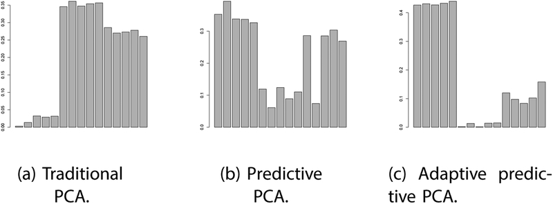
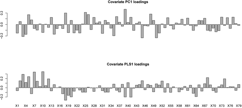
Figure 1 shows the pollutant PC1 loadings obtained from traditional PCA, predictive PCA, and adaptive predictive PCA methods for one simulated training dataset. The traditional PCA algorithm does not take into account the dependence of pollutants on GIS covariates. Therefore the first pollutant PC identified by the traditional PCA method is not the first true pollutant PC as indicated by the low loadings of the first 5 pollutants in Figure 1a. That same figure indicates that the first pollutant PC identified by the traditional PCA method is a mixture of true PC2 and true PC3. In contrast, the predictive PCA algorithm does take into account the dependence on GIS covariates; however it pre-selects GIS covariate PCs to guide pollutant PC identification and the pre-selection is done independent of the pollutant data. So the predictive PCA method fails to identify PC1 correctly as well; it identifies PC1 to be a mixture of true PC1 and true PC3 (Figure 1b). The adaptive predictive PCA algorithm chooses GIS covariates taking into account their relationship with the pollutant data. Recall that the first true pollutant PC only depends on a few (8) of all 79 available GIS covariates with covariates numbered 5, 7 and 10 having the largest β values (Table 1). We see in Figure 2 that those 8 covariates and especially covariates numbered 7 and 10, do have more prominent loadings when we use the adaptive predictive PCA algorithm vs. the predictive PCA algorithm, which leads that algorithm to identify true pollutant PC1 correctly (Figure 1c) and further produce better predictions of pollutant PC1 at unobserved locations.
Figure 1:
For one simulated dataset with uncorrelated covariates: PC1 loadings for the 15 pollutant constituents. There is one bar for each pollutant.
Figure 2:
The first component of covariate loadings for predictive PCA, and for adaptive predictive PCA for pollutant PC1: for the simulation scenario with uncorrelated covariates. Note the difference in the axis scales: bottom figure axis maximum is greater than 0.2.
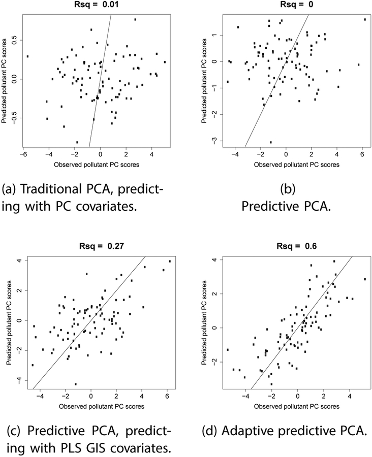
Figure 3 shows scatterplots of observed vs. predicted pollutant PC scores for the test locations; the prediction improves from the traditional PCA method to the adaptive predictive PCA method. Note that Figures 3b and 3c are based on models that use the same pollutant loadings but use GIS covariate PCs and covariate PLS components respectively for prediction. Figures 3a and 3b are based on models that use different pollutant loadings but both use covariate PCs for prediction. For this simulation scenario, the first pollutant PC (PC1) obtained using the predictive PCA algorithm is not predictable (R2 = 0.01 Table 2). Predictability improves when we use PLS GIS covariates based on that PC at observed locations to predict the PC at new locations (R2 increased from 0.01 to 0.42 Table 2). Using the adaptive predictive PCA algorithm, R2 further increased from 0.42 to 0.61 (Table 2). For PC2, using partial least squares to predict the pollutant PC obtained from the predictive PCA algorithm improved the predictability (R2 increased from 0.01 to 0.53); using the adaptive predictive PCA algorithm yields no further improvement (Table 2). The third PC (PC3) is not predictable at new locations in this simulation design (Table 2).
Figure 3:
For one simulated dataset with uncorrelated covariates: Observed vs. predicted pollutant PC1 scores. The lines are 1–1 lines.
Table 2:
Mean R2 for the first three pollutant PCs from 100 simulated datasets. The standard errors are all less than 0.04. Simulation scenario 1 has uncorrelated GIS covariates. Simulation scenario 2 has correlated GIS covariates.
| Simulation scenario 1 | Simulation scenario 2 | ||||||
|---|---|---|---|---|---|---|---|
| R2 | R2 | ||||||
| PC1 | PC2 | PC3 | PC1 | PC2 | PC3 | ||
| Traditional PCA GIS PC prediction | 0.03 | 0.01 | 0.00 | 0.78 | 0.62 | 0.18 | |
| Predictive PCA | 0.01 | 0.01 | 0.01 | 0.85 | 0.72 | 0.05 | |
| Predictive PCA GIS PLS prediction | 0.42 | 0.53 | 0.05 | 0.87 | 0.74 | 0.03 | |
| Adaptive predictive PCA | 0.61 | 0.52 | 0.01 | 0.84 | 0.76 | 0.00 | |
Recall that in the PCA algorithms, there are two steps – obtaining the pollutant PC loadings at training locations, and predicting pollutant PC scores at test locations. The predictive PCA algorithm uses the same GIS covariates for both steps as does the adaptive predictive PCA algorithm. However it is also possible to use different covariates in the two steps. (The traditional PCA algorithm does not use any GIS covariates to obtain pollutant PC loadings, the pollutant PC scores are then predicted at test locations using GIS covariates.) We can use the 15 true GIS covariates used to simulate the pollutant data, we can use all 79 available covariates, we can use PCs of the 79 covariates, or we can use PLS covariates obtained using the 79 covariates and training data pollutant PCs. In Table S1 in online Supplementary Material, we present the R2 values using each of those four possible GIS covariate choices. Note that the best R2 is obtained by using the predictive PCA algorithm with true GIS covariates in both steps, however the true GIS covariates affecting the pollutant data will be unknown in reality. Compared to predictive PCA using true covariates to obtain the loadings and PLS covariates in the prediction step, the adaptive predictive PCA algorithm yields the same predictability without using the true covariates. The traditional PCA algorithm produces the same R2 values as the predictive PCA algorithm using all 79 GIS covariates in the first step. This is because, we have 80 training data locations, so using 79 GIS covariates fails to constrain the pollutant loadings and the predictive PCA algorithm reduces to the traditional PCA algorithm.
4.2. Simulation scenario 2
The pollutants are simulated similarly as before. But now we use different GIS covariates – the covariates are simulated from the multivariate normal distribution such that the covariates influencing the first 5 pollutants, i.e., covariates numbered 1 to 10, are moderately correlated and the GIS covariates influencing pollutants 6 to 10, i.e., covariates numbered 11 to 15, are also moderately correlated.
As evident from Table 2, now the adaptive predictive PCA algorithm does not give better predictability of the PCs, rather it gives just the same amount of predictability as the predictive PCA algorithm or the predictive PCA algorithm with prediction using PLS GIS covariates. This is due to the correlated nature of the covariates influencing the pollutant PCs. The covariate PLS components used in the adaptive predictive PCA algorithm are very similar to the covariate PCs used in the predictive PCA algorithm (Figure S1 in online Supplementary Material shows the first components of each for the first pollutant PC). So the predictive PCA and adaptive predictive PCA algorithms produce very similar results. Figures S2 and S3 in the online Supplementary Material show the pollutant PC loadings and scatterplots of predicted vs observed pollutant PC scores for the first PC for this simulation scenario. Table S2 in the online Supplementary Material shows the R2 values using the four possible GIS covariate combinations in the two steps of the algorithms as described in the last paragraph of the previous subsection.
5. Data analysis
We use the data described in Section 2 to obtain principal components of PM2.5’s constituents, and evaluate predictability at new locations using leave-one-out cross validation.
Before analysis, we removed 2 locations with some missing pollutant observations and 5 locations where geographic covariate data were not available. We scale all pollutants by dividing them by the PM2.5 data. Then we log transform the pollutant data followed by mean centering and scaling by the respective pollutant standard deviations. The PM10 data were not used in analyses. So we have data at 142 locations for 20 scaled components of PM2.5.
All GIS covariates were preprocessed to remove covariates with identical values at all the 142 locations. We used 294 geographic covariates for the data analysis, and all covariates were mean centered and scaled by their respective standard deviations. To account for the spatial nature of the data, we also include some thin plate spline basis functions as covariates in our data analysis; similar to Jandarov et al. (2017) we use splines of 10 degrees of freedom. See Section 6 for a discussion on future work incorporating splines into the adaptive predictive PCA algorithm in a different way. In the predictive PCA algorithms we outlined in Section 3, we used the GIS covariates as predictors in a multiple linear regression model for prediction of pollutant PC scores. We note that the predictive PCA algorithm of Jandarov et al. (2017) uses universal kriging to predict pollutant PC scores at new locations.
5.1. Results
5.1.1. Pollutant PCs obtained using different PCA methods
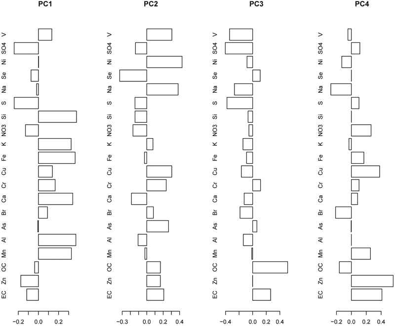
The first 4 pollutant PC loadings obtained from the dataset using the adaptive predictive PCA method are shown in Figure 4. The loadings for the first 4 pollutant PCs obtained from the dataset using all discussed PCA methods are shown in Figures S4 and S5 in online Supplementary Material. There are noticeable differences in the pollutant loadings obtained using the three PCA methods because in the different PCA methods, different GIS covariates have been used to obtain the loadings. The GIS covariate loadings (first 4 components) used in the predictive and the adaptive predictive PCA methods are shown in Figures S6, S7, S8, S9, S10 in online Supplementary Material. For ease of visualization, the GIS covariates have been grouped into categories, and each category contains covariates of the same type, possibly arising from different buffer size radii, e.g., population values at 500m, 1Km, 1.5Km, 2Km, 2.5Km, 3Km, 5Km, 10Km, and 15Km from the pollution monitoring location. Note that the predictive PCA method uses the same GIS covariates for all three pollutant PCs, but the adaptive predictive PCA method chooses a different set of GIS covariates for each pollutant PC. All PCA methods result in pollutant PC scores that are minimally correlated (correlations less than 0.1 except in one case; Table S3 in online Supplementary Material). PC1 and PC3 obtained from the adaptive predictive PCA method have a correlation of 0.27, however PC3 still explains a substantial amount (13%; Table 3) of the pollutant space variability.
Figure 4:
Loadings for first 4 pollutant PCs using the adaptive predictive PCA method on IMPROVE 2014 data.
Table 3:
Summary results for the first four pollutant PCs from IMPROVE 2014 data. The R2 have been obtained by leave one out cross validations. The values of variance explained by each PC have been obtained from the whole dataset.
| R2 | Variance explained | ||||||||||
|---|---|---|---|---|---|---|---|---|---|---|---|
| PC1 | PC2 | PC3 | PC4 | PC1 | PC2 | PC3 | PC4 | Total:4PCs | |||
| Traditional PCA GIS PC prediction | 0.55 | 0 | 0.33 | 0.52 | 32% | 17% | 14% | 9% | 73% | ||
| Predictive PCA | 0.55 | 0 | 0 | 0.33 | 32% | 16% | 9% | 12% | 69% | ||
| Predictive PCA GIS PLS prediction | 0.77 | 0.55 | 0.11 | 0.57 | 32% | 16% | 9% | 12% | 69% | ||
| Adaptive predictive PCA | 0.78 | 0.55 | 0.45 | 0.34 | 32% | 17% | 13% | 9% | 71% | ||
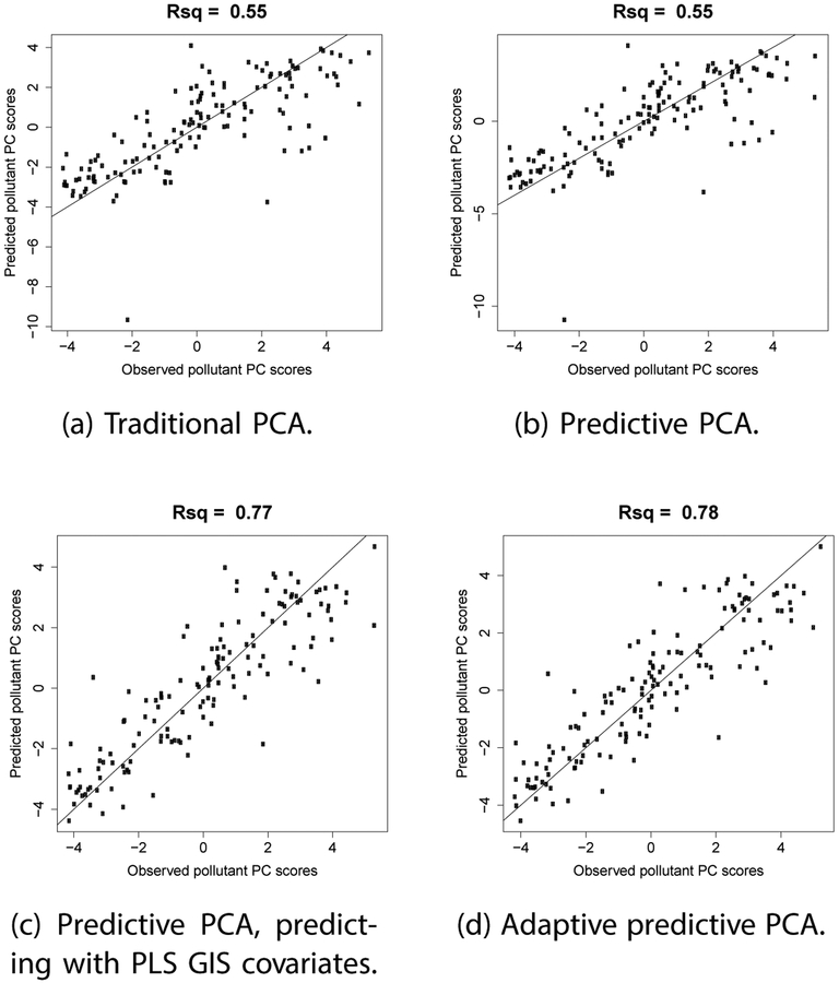
We see that the pollutant loadings obtained using the traditional PCA, the predictive PCA, and the adaptive predictive PCA methods are quite similar for PC1, i.e., PC1 is similar for all three methods (Figure S4 in online Supplementary Material). That is why predictability of PC1 is similar for the predictive PCA and the traditional PCA methods (cross validated R2 values are in Table 3, Figure 6) since both these methods use PC GIS covariates for prediction. Then we see an improvement in predicability when we use PLS GIS covariates for prediction of the PC1 obtained using the predictive PCA algorithm (Table 3, Figure 6). However there is no further improvement in predictability when we use the adaptive predictive PCA method since we get similar pollutant loadings as before.
Figure 6:
PC1: Scatterplots of prediction of pollutant PC scores doing leave one out cross validation for IMPROVE 2014 data. The lines are 1–1 lines.
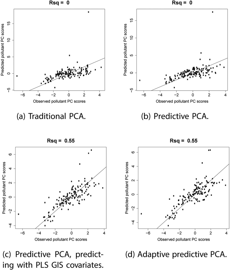
For PC2, there are some differences in pollutant loadings obtained using the traditional PCA, the predictive PCA, and the adaptive predictive PCA methods (Figure S4 in online Supplementary Material). However, neither the PC2 obtained using the traditional PCA method nor the PC2 obtained using the predictive PCA method is predictable using PC GIS covariates (Table 3, Figure 7). We again see an improvement in predictability when we use PLS GIS covariates for prediction. And similar to PC1, there is no further improvement in predictability when we use the adaptive predictive PCA method.
Figure 7:
PC2: Scatterplots of prediction of pollutant PC scores doing leave one out cross validation for IMPROVE 2014 data. The lines are 1–1 lines.
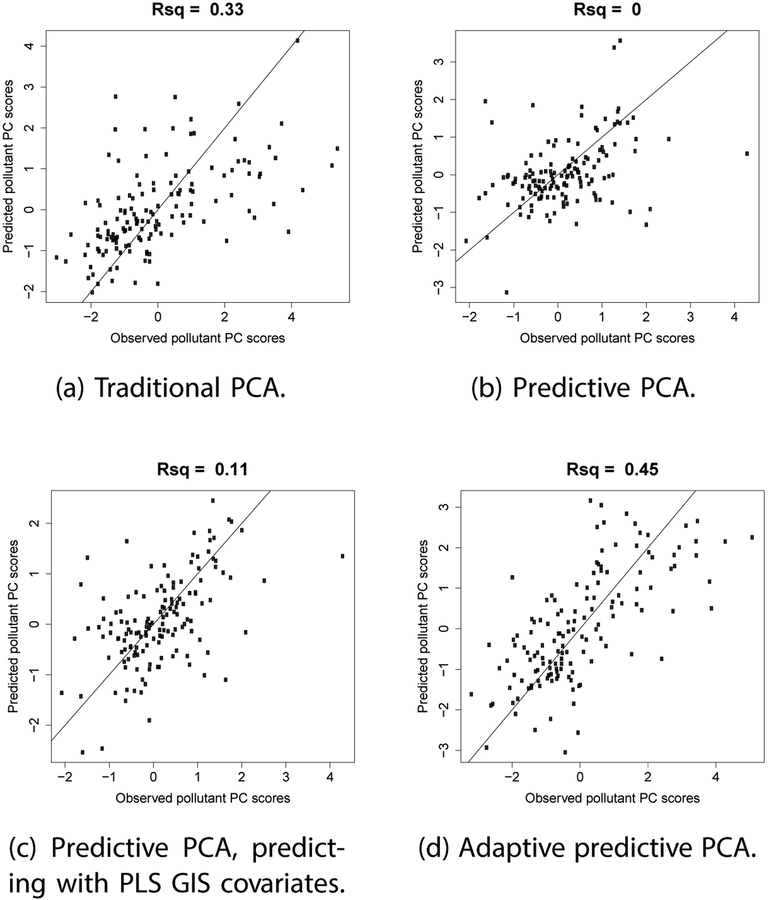
For PC3, the pollutant loadings obtained using the three PCA methods are most dissimilar (Figure S5 in online Supplementary Material), so predictability of PC3 is different using the different PCA methods; the adaptive predictive PCA method results in the maximum predictability (Table 3, Figure 8). This concurs with the fact that the GIS covariates for the predictive PCA method (Figure S6 in online Supplementary Material) are more dissimilar compared to the GIS covariates for PC3 from the adaptive predictive PCA method (Figure S9 in online Supplementary Material), than the GIS covariates for PC1 or PC2 from the adaptive predictive PCA method (Figures S7, S8 in online Supplementary Material). For this PC, the pre-selected GIS covariates in the predictive PCA method failed to pick a predictable pollutant PC, and predictability could not be improved by only using PLS GIS covariates in the prediction step.
Figure 8:
PC3: Scatterplots of prediction of pollutant PC scores doing leave one out cross validation for IMPROVE 2014 data. The lines are 1–1 lines.
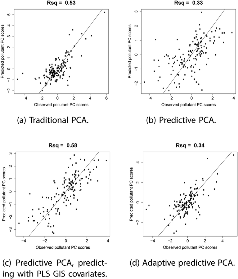
For PC4, the pollutant loadings obtained using the three PCA methods are dissimilar (Figure S5 in online Supplementary Material), and the predictability of PC4 is different using the different PCA methods as well (Table 3, Figure 9). Predictability for PC4 is maximum when we use PLS GIS covariates for prediction of the PC4 obtained by the predictive PCA algorithm.
Figure 9:
PC4: Scatterplots of prediction of pollutant PC scores doing leave one out cross validation for IMPROVE 2014 data. The lines are 1–1 lines.
The adaptive predictive PCA method yields the maximum predictability overall. The first 4 PCs obtained from this method also explain almost as much variance in the pollutant space explained by the first 4 PCs obtained from the traditional PCA method; additionally we note that the PCs obtained from the adaptive predictive PCA method are automatically ordered by amount of variance explained as well as by how predictable they are (Table 3). In the following subsection, we describe the PCs obtained from the adaptive predictive PCA method.
5.1.2. Composition of pollutant PCs
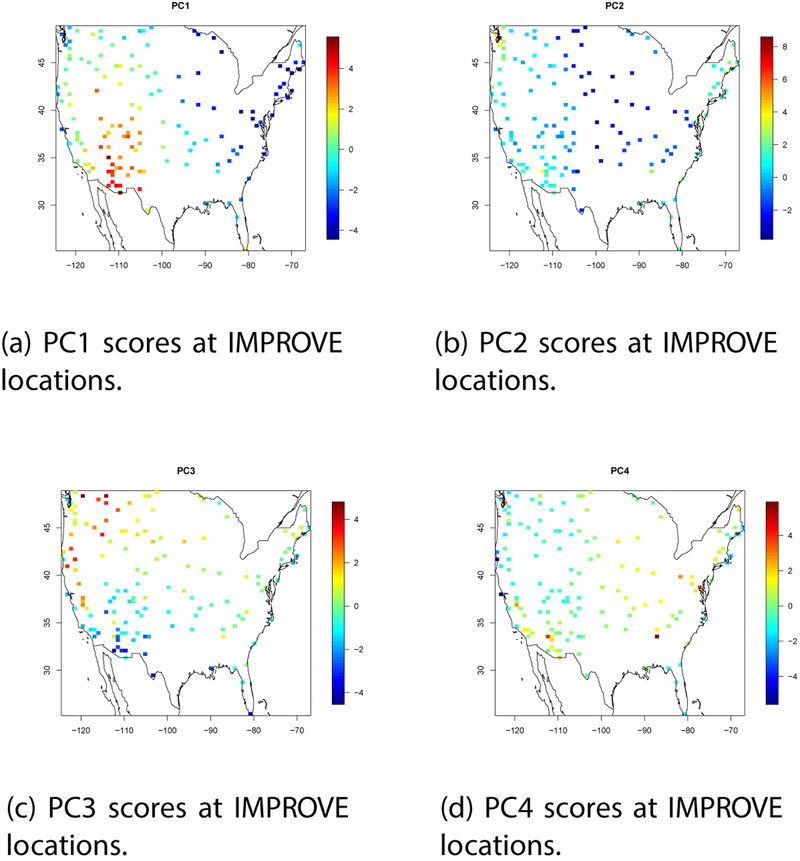
As mentioned earlier, the pollutant PC loadings obtained using the adaptive predictive PCA method are shown in Figure 4. Figure 9 shows the spatial distribution of the pollutant PC scores. The PCs can be interpreted as follows.
For PC1, the high positive loadings are possibly due to windblown dust and re-suspended soil (Si, Fe, K, Ca, Al) in the desert southwest (Tong et al., 2012; Clements et al., 2017; Thurston et al., 2011). The soil is not a main feature in the midwest and east due to more vegetative cover in those latter areas. The high negative loadings are possibly due to the absence of windblown dust in areas of high regional acid sulfate haze (SO4, NO3, Se) in the eastern U.S. (Hand et al., 2012).
For PC2, the high positive loadings are possibly due to ship emissions burning bunker fuel oil (Ni, V) along both coasts with additional contribution from seasalt (Na) (Kotchenruther, 2018; Thurston et al., 2011). The high negative loadings (NO3, Se) are possibly due to the absence of ship emission impacts in areas of high regional ammonium nitrate haze in the northern midwest (Coutant et al., 2003).
For PC3, the high positive loadings are possibly due to forest fires impacts (OC, EC, no metals) in the Pacific Northwest (Kaulfus et al., 2017; Thurston et al., 2011). The high negative loadings are possibly due to the absence of forest fire impacts in the desert southwest. The latter region is potentially impacted by sources in central Mexico including heavy oil processing (SO4)and a major volcano (V) (Gebhart et al., 2001; NASA Earth Observatory, 2018). Local Mexican sources along the U.S. Mexico border may also be impacting this latter region.
The loadings for PC4 are more difficult to interpret. The high positive loadings are possibly due to traffic emissions (EC) including brake (Cu) and tire wear (Zn) (Kueken et al., 2013; Oakes et al., 2016) in more populous regions of the U.S.
6. Discussion
For datasets where GIS covariates influence the pollutants but do not explain the covariate space variance, the existing predictive PCA algorithm (Jandarov et al., 2017) using PC GIS covariates is not advisable. The adaptive predictive PCA algorithm uses PLS regression iteratively to identify those GIS covariate profiles which affect the pollutant PCs. So when pollutants truly depend on GIS covariates, especially linearly, we get pollutant PCs which are better predictable at new locations using those PLS GIS covariates. The pollutant PCs can then be used in an effect modifier model to investigate health outcome changes due to different constituents of PM2.5; health-pollution associations can change depending on the composition of PM2.5 so this model is of great interest.
We have used partial least squares regression and principal components analysis. Various other unsupervised learning techniques for dimension reduction could potentially be used in the context of dimension reduction of multicomponent pollution data incorporating covariates; these techniques include clustering, nonlinear dimension reduction, independent component analysis, etc. Keller et al. (2017) developed a predictive k-means procedure; they used covariate data to cluster multicomponent pollutants and then performed spatial prediction of cluster membership at unobserved locations.
We have included spatial smoothing splines as covariates, and have treated the observed geographic covariates and splines in the same way. Future work will explore how to incorporate splines into the adaptive predictive PCA algorithm so that the splines are pre-specified as covariates, and the algorithm chooses PLS profiles only from the geographic covariates. In this context, we note that there are other ways to treat spatial structure in the data, for example, by performing universal kriging. Additionally, modifications of the PCA technique have been designed that account for spatial correlation in the data, e.g., geographically weighted PCA (Fotheringham et al. 2003), and spatial PCA (Jombart et al. 2008, Demšar et al. 2013). Our adaptive predictive PCA algorithm can potentially also be modified to handle spatiotemporal pollutant data.
The observed pollutant data in many cases contain missing values, e.g., some locations may have some missing pollutant components; the adaptive predictive principal component algorithm in its current form will not work with missing data.
Jandarov et al. (2017) developed the sparse predictive PCA method which leads to a large number of the pollutants having zero loadings; the PC scores then only consist of the pollutants with non-zero loadings. This makes it easier to interpret the PC scores. A sparse adaptive predictive PCA algorithm can be similarly developed by incorporating a penalty term for sparsity in the minimization algorithm.
Additional information and supporting material for this article is available online at the journal’s website.
Supplementary Material
Figure 5:
Scores for first 4 pollutant PCs using the adaptive predictive PCA method on IMPROVE 2014 data.
Acknowledgements
This paper was made possible by NIH/NIEHS grants 1R21ES024894 and T32ES015459, and NIH grant 5UG3OD023271. The contents of this paper are solely the responsibility of the authors and do not necessarily represent the official views of the National Institutes of Health-National Institute of Environment Health Sciences.
References
- Achilleos S, Kioumourtzoglou MA, Wu CD, Schwartz JD, Koutrakis P and Papatheodorou SI (2017). Acute effects of fine particulate matter constituents on mortality: A systematic review and meta-regression analysis. Environment International, 109, 89–100. [DOI] [PMC free article] [PubMed] [Google Scholar]
- Badaloni C, Cesaroni G, Cerza F, Davoli M, Brunekreef B and Forastiere F (2017). Effects of long-term exposure to particulate matter and metal components on mortality in the Rome longitudinal study. Environment International, 109, 146–154. [DOI] [PubMed] [Google Scholar]
- Bell ML, Dominici F, Ebisu K, Zeger SL, and Samet JM (2007). Spatial and temporal variation in PM(2.5) chemical composition in the United States for health effects studies. Environmental Health Perspectives, 115(7), 989–995. [DOI] [PMC free article] [PubMed] [Google Scholar]
- Bergen S, Sheppard L, Sampson PD, Kim SY, Richards M, Vedal S, … and Szpiro AA (2013). A national prediction model for PM2. 5 component exposures and measurement errorcorrected health effect inference. Environmental Health Perspectives, 121(9), 1017–1025. [DOI] [PMC free article] [PubMed] [Google Scholar]
- Brook RD, Rajagopalan S, Pope CA, Brook JR, Bhatnagar A, Diez-Roux AV, … Kaufman JD (2010). Particulate matter air pollution and cardiovascular disease: An update to the scientific statement from the American Heart Association. Circulation, 121(21), 2331–2378. [DOI] [PubMed] [Google Scholar]
- Clements AL, Fraser MP, Upadhyay N, Herckes P, Sundblom M, Lantz J and Solomon PA (2017). Source identification of coarse particles in the Desert Southwest, USA using Positive Matrix Factorization. Atmospheric Pollution Research, 8(5), 873–884. [DOI] [PMC free article] [PubMed] [Google Scholar]
- Coutant BW, Engel-Cox J and Swinton KE (2003). Compilation of existing studies on source apportionment for PM2.5 Technical report, Office of Air Quality Planning and Standards, USEPA, Washington, DC. [Google Scholar]
- Demšar U, Harris P, Brunsdon C, Fotheringham AS, and McLoone S (2013). Principal component analysis on spatial data: an overview. Annals of the Association of American Geographers, 103(1), 106–128. [Google Scholar]
- Dominici F, Peng R, Barr CD, and Bell ML (2010). Protecting Human Health from Air Pollution: Shifting from a Single-Pollutant to a Multi-pollutant Approach. Epidemiology, 21(2), 187–194. [DOI] [PMC free article] [PubMed] [Google Scholar]
- Fakhri AA, Ilic LM, Wellenius GA, Urch B, Silverman F, Gold DR, and Mittleman MA (2009). Autonomic Effects of Controlled Fine Particulate Exposure in Young Healthy Adults: Effect Modification by Ozone. Environmental Health Perspectives, 117(8), 1287–1292. [DOI] [PMC free article] [PubMed] [Google Scholar]
- Fotheringham AS, Brunsdon C, and Charlton M (2003). Geographically Weighted Regression: the analysis of spatially varying relationships. John Wiley and Sons. [Google Scholar]
- Gebhart KA, Kreidenweis SM, and Malm WC (2001). Back-trajectory analyses of fine particulate matter measured at Big Bend National Park in the historical database and the 1996 scoping study. Science of the Total Environment, 276(1–3), 185–204. [DOI] [PubMed] [Google Scholar]
- Gold DR, Litonjua A, Schwartz J, Lovett E, Larson A, Nearing B, … Verrier R (2000). Ambient Pollution and Heart Rate Variability. Circulation, 101(11), 1267–1273. [DOI] [PubMed] [Google Scholar]
- Hand JL, Schichtel BA, Pitchford M, Malm WC and Frank NH (2012). Seasonal composition of remote and urban fine particulate matter in the United States. Journal of Geophysical Research: Atmospheres, 117 (D5). [Google Scholar]
- Hsu CY, Chiang HC, Chen MJ, Chuang CY, Tsen CM, Fang GC, … Chen YC (2017). Ambient PM2.5 in the residential area near industrial complexes: Spatiotemporal variation, source apportionment, and health impact. Science of the Total Environment, 590, 204–214. [DOI] [PubMed] [Google Scholar]
- Jandarov RA, Sheppard LA, Sampson PD, and Szpiro AA (2017). A novel principal component analysis for spatially misaligned multivariate air pollution data. J. R. Stat. Soc. C, 66(1): 3–28. [DOI] [PMC free article] [PubMed] [Google Scholar]
- Jombart T, Devillard S, Dufour AB, and Pontier D (2008). Revealing cryptic spatial patterns in genetic variability by a new multivariate method. Heredity, 101(1), 92–103. [DOI] [PubMed] [Google Scholar]
- Katsouyanni K, Touloumi G, Samoli E, Gryparis A, Le Tertre A, Monopolis Y, … Schwartz J (2001). Confounding and effect modification in the short-term effects of ambient particles on total mortality: results from 29 European cities within the APHEA2 project. Epidemiology, 12(5), 521–531. [DOI] [PubMed] [Google Scholar]
- Kaulfus AS, Nair U, Holmes CD and Landing WM (2017). Mercury wet scavenging and deposition differences by precipitation type. Environmental Science and Technology, 51(5), 2628–2634. [DOI] [PubMed] [Google Scholar]
- Keller JP, Drton M, Larson T, Kaufman JD, Sandler DP, and Szpiro AA (2017). Covariate-adaptive clustering of exposures for air pollution epidemiology cohorts. The Annals of Applied Statistics, 11(1), 93. [DOI] [PMC free article] [PubMed] [Google Scholar]
- Kim JO, and Mueller CW (1978). Factor Analysis: Statistical methods and practical issues (Vol. 14). New York: Sage. [Google Scholar]
- Keuken MP, Moerman M, Voogt M, Blom M, Weijers EP, Röckmann T and Dusek U (2013). Source contributions to PM2.5 and PM10 at an urban background and a street location. Atmospheric Environment, 71, 26–35. [Google Scholar]
- Kotchenruther RA (2017). The effects of marine vessel fuel sulfur regulations on ambient PM2.5 at coastal and near coastal monitoring sites in the US. Atmospheric Environment, 151, 52–61. [Google Scholar]
- Jolliffe IT (1986) Principal Component Analysis. New York: Springer. [Google Scholar]
- Miller KA, Siscovick DS, Sheppard L, Shepherd K, Sullivan JH, Anderson GL, and Kaufman JD (2007). Long-term exposure to air pollution and incidence of cardiovascular events in women. New England Journal of Medicine, 356(5), 447–458. [DOI] [PubMed] [Google Scholar]
- NASA Earth Observatory. (2018). The Ups and Downs of Sulfur dioxide in North America. https://earthobservatory.nasa.gov/IOTD/view.php?id=90276. [Google Scholar]
- Oakes MM, Burke JM, Norris GA, Kovalcik KD, Pancras JP and Landis MS (2016). Near-road enhancement and solubility of fine and coarse particulate matter trace elements near a major interstate in Detroit, Michigan. Atmospheric Environment, 145, 213–224. [Google Scholar]
- Pascal M, Falq G, Wagner V, Chatignoux E, Corso M, Blanchard M, … Larrieu S (2014). Short-term impacts of particulate matter (PM10, PM102.5, PM2.5) on mortality in nine French cities. Atmospheric Environment, 95, 175–184. [Google Scholar]
- Peel JL, Tolbert PE, Klein M, Metzger KB, Flanders WD, Todd K, … Frumkin H (2005). Ambient Air Pollution and Respiratory Emergency Department Visits. Epidemiology, 16(2), 164–174. [DOI] [PubMed] [Google Scholar]
- Pope CA, Burnett RT, Thurston GD, Thun MJ, Calle EE, Krewski D, and Godleski JJ (2004). Cardiovascular mortality and long-term exposure to particulate air pollution: epidemiological evidence of general pathophysiological pathways of disease. Circulation, 109(1), 71–77. [DOI] [PubMed] [Google Scholar]
- Samoli E, Atkinson RW, Analitis A, Fuller GW, Beddows D, Green DC, Mudway IS, Harrison RM, Anderson HR and Kelly FJ (2016). Differential health effects of short-term exposure to source-specific particles in London, UK. Environment International, 97, 246–253. [DOI] [PubMed] [Google Scholar]
- Shen H, and Huang JZ (2008). Sparse principal component analysis via regularized low rank matrix approximation. J. Multiv. Anal, 99, 1015–1034. [Google Scholar]
- Tao Y, Huang W, Huang X, Zhong L, Lu SE, Li Y, Zhu T (2012). Estimated acute effects of ambient ozone and nitrogen dioxide on mortality in the Pearl River Delta of southern China. Environmental Health Perspectives, 120(3), 393–398. [DOI] [PMC free article] [PubMed] [Google Scholar]
- Thurston GD, Burnett RT, Turner MC, Shi Y, Krewski D, Lall R, Ito K, Jerrett M, Gapstur SM, Diver WR and Pope CA III (2016). Ischemic heart disease mortality and long-term exposure to source-related components of US fine particle air pollution. Environmental Health Perspectives, 124(6), p.785. [DOI] [PMC free article] [PubMed] [Google Scholar]
- Thurston GD, Ito K and Lall R (2011). A source apportionment of US fine particulate matter air pollution. Atmospheric Environment, 45(24), 3924–3936. [DOI] [PMC free article] [PubMed] [Google Scholar]
- Tian L, Zeng Q, Dong W, Guo Q, Wu Z, Pan X, Li G and Liu Y (2017). Addressing the source contribution of PM2.5 on mortality: an evaluation study of its impacts on excess mortality in China. Environmental Research Letters, 12(10), 104016. [Google Scholar]
- Tolbert PE, Klein M, Peel JL, Sarnat SE, and Sarnat JA (2007). Multipollutant modeling issues in a study of ambient air quality and emergency department visits in Atlanta. Journal of Exposure Science and Environmental Epidemiology, 17 Suppl 2, S29–35. [DOI] [PubMed] [Google Scholar]
- Tong DQ, Dan M, Wang T and Lee P, (2012). Long-term dust climatology in the western United States reconstructed from routine aerosol ground monitoring. Atmospheric Chemistry and Physics, 12(11), 5189–5205. [Google Scholar]
- Vedal S, and Kaufman JD (2011). What does multi-pollutant air pollution research mean? American Journal of Respiratory and Critical Care Medicine, 183(1), 3–4. [DOI] [PubMed] [Google Scholar]
- Weichenthal S, Villeneuve PJ, Burnett RT, van Donkelaar A, Martin RV, Jones RR, … Hoppin JA (2014). Long-term exposure to fine particulate matter: association with nonaccidental and cardiovascular mortality in the agricultural health study cohort. Environmental Health Perspectives, 122(6), 609–615. [DOI] [PMC free article] [PubMed] [Google Scholar]
- Wold H (1985). Partial least squares Encyclopedia of statistical sciences, 6, 581–591. New York: Wiley. [Google Scholar]
- Zanobetti A, Franklin M, Koutrakis P, and Schwartz J (2009). Fine particulate air pollution and its components in association with cause-specific emergency admissions. Environmental Health, 8, 58. [DOI] [PMC free article] [PubMed] [Google Scholar]
Associated Data
This section collects any data citations, data availability statements, or supplementary materials included in this article.


