Abstract
Recently, anovel coronavirus disease (COVID-19) has become a serious concern for global public health. Infectious disease outbreaks such as COVID-19 can also significantly affect the sustainable development of urban areas. Several factors such as population density and climatology parameters could potentially affect the spread of the COVID-19. In this study, a combination of the virus optimization algorithm (VOA) and adaptive network-based fuzzy inference system (ANFIS) was used to investigate the effects of various climate-related factors and population density on the spread of the COVID-19. For this purpose, data on the climate-related factors and the confirmed infected cases by the COVID-19 across the U.S counties was used. The results show that the variable defined for the population density had the most significant impact on the performance of the developed models, which is an indication of the importance of social distancing in reducing the infection rate and spread rate of the COVID-19. Among the climatology parameters, an increase in the maximum temperature was found to slightly reduce the infection rate. Average temperature, minimum temperature, precipitation, and average wind speed were not found to significantly affect the spread of the COVID-19 while an increase in the relative humidity was found to slightly increase the infection rate. The findings of this research show that it could be expected to have slightly reduced infection rate over the summer season. However, it should be noted that the models developed in this study were based on limited one-month data. Future investigation can benefit from using more comprehensive data covering a wider range for the input variables.
Keywords: COVID-19;Climatology, Adaptive neuro-fuzzy inference system, Virus optimization algorithm
1. Introduction
The rapid spread of the novel coronavirus disease (i.e., COVID-19), which was started since the late December 2019, has become a serious global issue [1], [2], [3], [4]. As of April 28, 2020, the official reports indicated more than 3,000,000 infected cases and over 217,000 confirmed deaths attributed to the COVID-19 complications. In addition, the rapid spread of the COVID-19 has affected 210 countries worldwide. The official statistics shows that with more than 1,000,000 infected cases and over 59,000 confirmed deaths, the USA is one of the countries where the rapid widespread of COVID-19 has seriously threatened the life of people. Several factors could potentially affect the spread and transmission rates of the viruses including population density and climatology parameters (e.g., wind speed, humidity, precipitation, and temperature) [5], [6], [7], [8], [9], [10]. The sustainable development of urban areas necessities the investigation of the effects of these factors on the transmission rate of the viruses to have an efficient spatial organization of the resident areas. Different climate conditions have been reported to affect the transmission rate of viruses differently. The transmission rate of some viruses such as HIV/AIDS are not affected by climate parameters. The HIV/AIDS virus never leaves the host's internal condition as it transfers through sexual intercourse, blood transfusions, or during pregnancy or breastfeeding from mother to child. For the flu virus, dry and cold climates have been found as favorable conditions to spread the virus, while temperatures above 30˚C halt its transmission [11]. With regard to the MERS-CoV, the widespread occurrence of this virus was reported to be between April to August, when high temperature is dominant [12]. Moreover, high ultraviolet index, low relative humidity, and low wind speeds were found as favorable conditions for the spread of the MERS-CoV [12].In terms of the spread of the COVID-19, lower spread rate is attributed to warm and humid climate conditions in China [5]. However, a warm and humid climate does not seem to completely stop the spread of the COVID-19 [6].
An accurate model to investigate the climatology-related determinants of the spread of COVID-19 can be helpful for the sustainable development of the urban areas. Machine learning (ML) techniques and algorithms, due to their exceptional ability in knowledge processing, have been proven to provide accurate models in many fields of science and engineering [13], [14], [15]. ML techniques have also been widely used in the study of developing models for the prediction of outbreak [16,17]. Table 1 provides some examples of the previous studies on using the ML techniques for the prediction of the disease outbreak.
Table 1.
Examples of the ML techniques for the prediction of outbreak.
| Outbreak infection | ML technique | Main findings | Reference |
|---|---|---|---|
| Dengue | Naïve Bayes and adopted multi-regression | A high relative humidity accompanied with a temperature of 30-35 ˚C is a favorable condition for the spread of dengue. | [18] |
| Dengue | Neural network | Integration ofremote sensing data, a ML technique and spatiotemporal analysis provided a climate-based predictive model with high accuracy for the spread of dengue. | [19] |
| Oyster norovirus | Neural network | With 2-day lead time, the developed model can predict oyster norovirus outbreaks. | [20] |
| Oyster norovirus | Genetic programming and neural network | Climate-related factors were found to play a significant role in the cause likelihood of oyster norovirus outbreaks. | [21,22] |
| Oyster norovirus | Probability-based artificial neural network | Climate-related factors such as temperature, wind, salinity, and rainfall were found as the determinants of norovirus outbreaks. Moreover, depth of water in an oyster bed was found as the most significant factor in the developed model. | [23] |
| Swine fever | Random forests | Precipitation and driest month had the most significant effects on the outbreak of African swine fever. | [24] |
| Influenza | Neural network, random forests, support vector machine | The random forests time series provided better statistical fit than support vector machine and artificial neural network in modeling weekly influenza like illness. | [25] |
| COVID-19 | Genetic programming | The predictive models based on genetic programming provide high accuracy in determining the factors that affect the infection rate of COVID-19. | [26] |
In this study, adaptive network-based fuzzy inference system (ANFIS) and virus optimization algorithm (VOA) were used to investigate the effects of climate-related factors on the spread of COVID-19. For this purpose, a dataset containing the information on COVID-19 spread across the U.S. counties was used. A sensitivity analysis was also performed to identify the most significant factors affecting the spread of the COVID-19.
2. Data collection
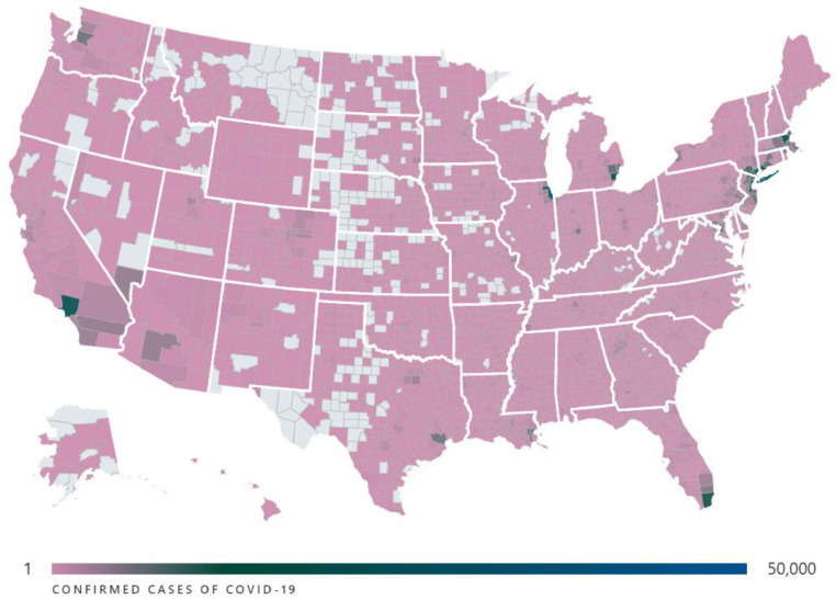
The data used in this research to study the climate-related determinants of the spread of the COVID-19 in the U.S. was collected from various sources. The distribution of the confirmed infected cases by the COVID-19 across the country was provided by the USAFacts (2020) (Fig. 1 ) [27]. Information about the average temperature, maximum temperature, minimum temperature, and precipitation was obtained from the NOAA (2020) [28]. It should be noted that the data for the month of March was used for these variables. Data for the information on the average annual humidity, average annual wind speed, and population was collected from the USA.com (2020) [29]. The population density, as one of the input variables, indicates the number of people per squared miles. The only output variable in this study was the infection rate, which was defined as the number of confirmed infected cases over the days of infection. The counties with less than 10 confirmed infected cases were removed from the analysis to reduce the errors related to the random effects of these counties. Overall, a total of 1657 counties were used to model the spread of the COVID-19. The descriptive statistics of the input and output variables are given in Table 2 .
Fig. 1.
COVID-19 map by county [27].
Table 2.
Statistical indicators of the input and output variables.
| Input variables |
||||||||
|---|---|---|---|---|---|---|---|---|
| Statistical indicators | Population density | Average temperature | Maximum temperature | Minimum temperature | Precipitation | Wind speed | Humidity | Output variable Infection rate |
| Minimum | 1.4016 | 9.8000 | 19.6000 | -0.1000 | 0.0200 | 7.3000 | 63.3700 | 0.1266 |
| Maximum | 71340.6045 | 76.4000 | 86.4000 | 67.8000 | 10.7300 | 34.5000 | 87.4100 | 913.5435 |
| Average | 603.5411 | 9.4837 | 9.7883 | 9.2526 | 1.8044 | 2.1282 | 2.5300 | 15.2436 |
| Standard deviation | 2439.0458 | 11.1792 | 11.5296 | 10.9617 | 2.1978 | 2.8359 | 3.2920 | 55.1694 |
| Skewness | 19.3877 | 0.0355 | 0.0093 | 0.0552 | 0.4957 | 0.5096 | -0.3014 | 11.0189 |
| Kurtosis | 484.5741 | -0.7785 | -0.7959 | -0.7015 | -0.3631 | 2.5896 | 0.8900 | 140.0478 |
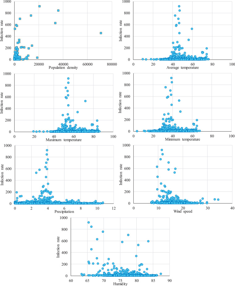
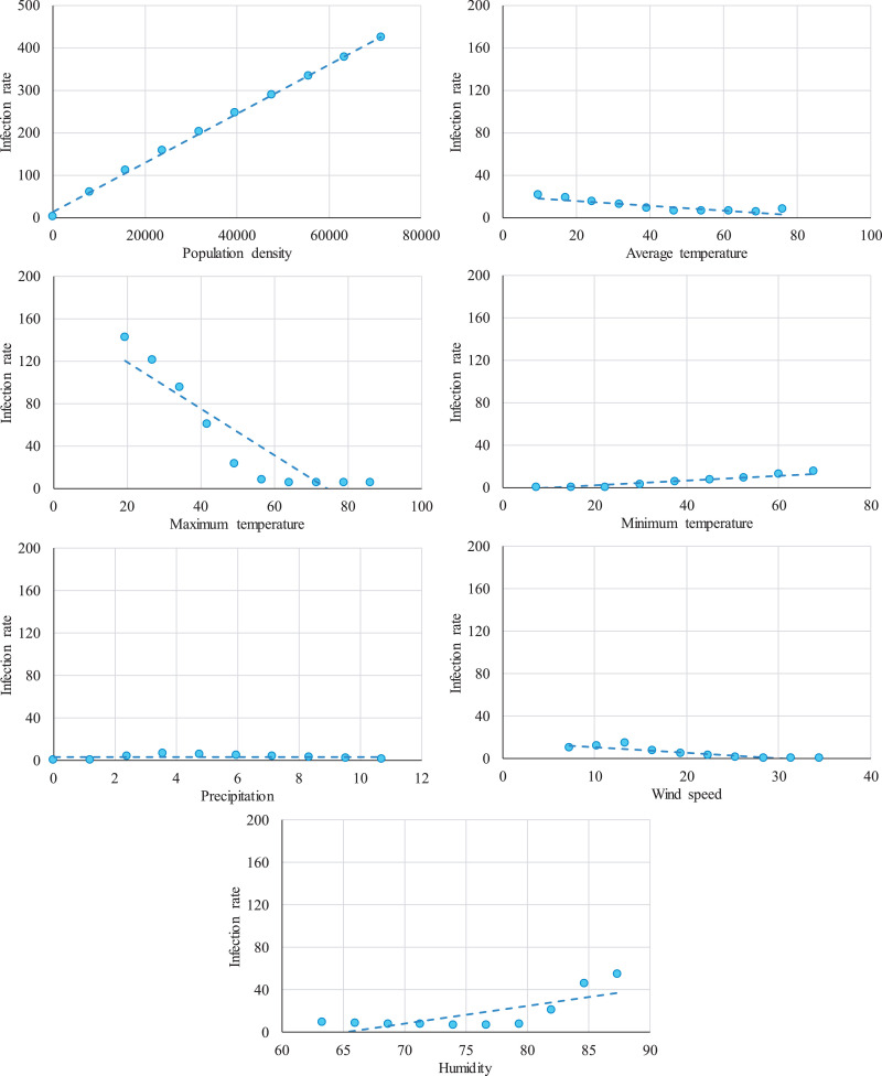
In order to further demonstrate the distribution of the climatology variables in the gathered database, Fig. 2 shows the infection rate, as the indicator of the COVID-19 outbreak, versus the seven input variables. As depicted in this figure, there is a direct relationship between the infection rate and the population density. However, the changing range of the infection rate for a given population density is remarkable. In the case of the other six input variables, there is not an apparent trend between them and the infection rate, which makes the modeling of the COVID-19 outbreak more difficult.
Fig. 2.
The relationship between the infection rate and the climatology variables.
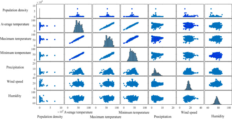
The pairwise relationships between the input variables are depicted in Fig. 3 . As expected, the correlation between the average, minimum and maximum temperatures are high. However, because of the non-parametric nature of the ML methods, all these variables are considered in the proposed model. Additionally, the other input variables do not have high correlation with each other.
Fig. 3.
The pairwise relationship between the climatology variables.
3. Proposed machine learning method
To introduce the proposed machine learning method, the virus optimization algorithm (VOA) is described at first, followed by the main concepts of the adaptive neuro-fuzzy inference system (ANFIS). Finally, the incorporation of the ANFIS and VOA is explained as the suggested model for the determination of the influence of climatology factors on the spread of the COVID-19.
3.1. Virus optimization algorithm (VOA)
All viruses with different sources include an envelope, a protein coat, and a genetic element that can infect the cells of human beings. By changing the metabolism of the host cell, which is the infected cell by the viruses, the viruses can reproduce a considerable number of new viruses, and it can cause the death of the cell. The rate of virus replication depends totally on the interaction between the virus and the cell, and it is higher for potent viruses with powerful RNA and DNA structures, like the COVID-19. By producing antibodies, the defense system of the body acts after entering the virus into the cell, protects the cell against the virus, and tries to prevent the death of the host cell. Due to the severity of the virus, probably, the produced antibodies could not protect the host cell and lead to its death.
The VOA is a population-based optimization algorithm in which each virus that attacks a host cell is a candidate solution for the optimization problem [30]. There are three main steps in the VOA, including initialization, replication, and maintenance phases. In the initialization phase, the primitive viruses are randomly generated, evaluated, and sorted from the best to the worst virus. Then, all created viruses are classified into strong viruses (SVs) and the common viruses (CVs) in which the SVs and the CVs are the best and the worst viruses, respectively. Next, the replication phase starts by producing new viruses by changing the SVs and CVs using the following equations:
| (1) |
| (2) |
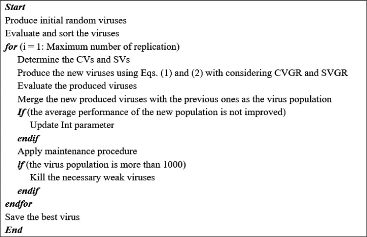
where , CVij and SVij are the jth dimension of the ith new virus, the common virus, and the strong virus, respectively; rand() is a number between zero and one; and Int is a parameter which set to one at the beginning of the algorithm. If the average performance of all viruses in the current replication is less than that in the previous replication, one unit is added to Int. The new viruses generated by CVs keep the exploration ability of the VOA, while those produced by SVs maintain the exploitation capacity of the algorithm. If the generated value for any dimension of a new virus is out of the allowable range, the process is repeated so that an allowable value is generated. At the beginning of the VOA, the focus of the algorithm is on the identification of new viruses in the decision space. During the replications and with increasing the Int value, the changes in the produced virus decreases, and the neighbors of the SVs, as the best viruses in the host cell, are exploited. The number of generated viruses from CVs and SVs are determined using two control parameters called common viruses’ growth rate (CVGR) and strong viruses’ growth rate (SVGR), respectively. Afterward, the newly produced viruses are evaluated, merged with the previous viruses, and sorted. In the VOA, the number of existing viruses is dynamic and can vary from one replication to another one. The third phase of the VOA is the maintenance procedure in which several viruses (nkv) are killed to survive the host cell. The number of killed viruses in each replication is defined as a random integer between one and the number of viruses in the cell minus the number of SVs. To select the candidate viruses to be killed, more chance is given to the worst viruses, which are the weakest ones. Based on the scientific experiments, the average capacity of a host cell is about 1000 viruses. It means that if the number of viruses in a host exceeds this threshold, more viruses should be killed to keep the capacity of the cell. The three main phases of the VOA are repeated until the termination condition of the algorithm is met. The maximum number of the replication is used as the termination condition in this study. The Pseudo-code of the VOA is shown in Fig. 4 .
Fig. 4.
The Pseudo-code of the VOA.
3.2. Adaptive network-based fuzzy inference system (ANFIS)
ANFIS is a ML method that benefits the fuzzy system in an adapted network structure [31]. This method is an extension of the TSK fuzzy system [32], which discovers the knowledge between input and output variables of a system using If-Then fuzzy rules. Each fuzzy rule consists of the antecedent and consequence parts in which the former part is presented as fuzzy inputs, and the latter one can be expressed as a linear combination of crisp input variables. Moreover, the fuzzy inputs in the antecedent part of a rule are aggregated with each other with AND logistic operator. The kth fuzzy rule (Rk) of a system with n input variables is as follows:
| (3) |
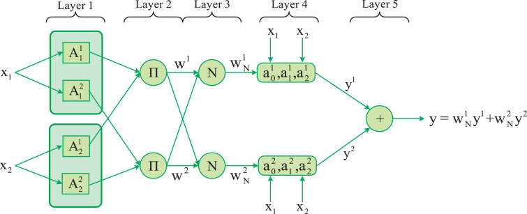
where xi and yk are the ith input variable and the output of kth fuzzy rule, respectively; is the membership function of the ith input variable related to the kth rule; is the regression coefficients in the antecedent part; and is its bias. Fig. 5 depicts an ANFIS structure with two input variables and two fuzzy rules. As illustrated in this figure, there are five layers in the ANFIS, and more explanation about the tasks of each layer are given in the followings:
Fig. 5.
An example of an ANFIS model with two input variables and two rules.
First layer: This layer is called the fuzzification layer in which the membership degrees of all membership functions for given input variables are calculated. Prior to computing the membership degrees, the membership functions of the input variables and the regression coefficients of the consequence parts of all fuzzy rules, as well as the number of the fuzzy rules, should be determined. The number of fuzzy rules in the ANFIS is set using subtractive clustering (SC) algorithm, as one of the fastest unsupervised training algorithms [33]. Moreover, the fuzzy c-means (FCM) clustering algorithm is served to determine the initial center and spread of Gaussian fuzzy membership functions of the input variables [34]. Additionally, the regression coefficients of the consequence parts of all fuzzy rules are the same and equal the regression coefficients achieved from the linear regression model fitted the existing data. After generating the initial fuzzy rule base, the training phase of the ANFIS begins in which the membership functions and regression coefficients are optimized in such a way that the error of the system minimized. The hybrid optimization algorithm is the most popular training algorithm of the ANFIS in which the least-squares method (LSM) is used to optimize the regression coefficients of fuzzy rules in the forward movement of information from the first layer to the fifth layer [35]. Meanwhile, the gradient descend (GD) algorithm is used to optimize the parameters related to the membership functions in the backward movement.
Second layer:After calculating the membership degrees of all membership functions for given input variables, the aggregated value of the antecedent part of each fuzzy rule is calculated, using the following equation, which shows the firing strength of the rule.
| (4) |
Third layer:The normalized weights of all rules are calculated using the following equation:
| (5) |
Fourth layer:Having the regression coefficients of all rules, the consequence value of each rule is calculated for given input variables, as follows:
| (6) |
Fifth layer:The output of the ANFIS model for given input variables is calculated as the weighted consequence values of all rules, formulated as follows:
| (7) |
3.3. Incorporated model of ANFIS and VOA
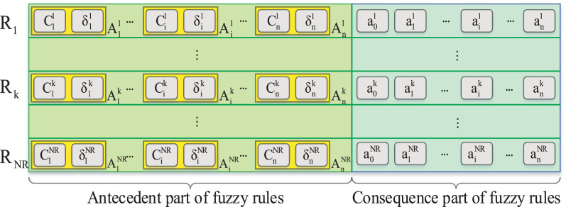
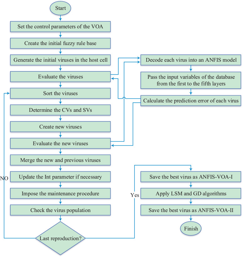
Trapping in the local optima is the critical drawback of the GD algorithm. The accuracy of this algorithm depends totally on the initial values of decision variables in the optimization problem. Therefore, serving VOA can be a good idea to optimize the centers and spreads of membership functions of input variables as well as the regression coefficients of the consequence parts of fuzzy rules in such a way to avoid the local optima through the exploration of searching space at the beginning of replications and also to converge to the optimal solution through the exploitation of the best existing solutions. In this regard, each virus in the VOA is represented as a matrix with the dimension of NR × (3 × n+1) in which n is the number of input variables, and NR is the number of rules in the rule base. A schematic representation of a virus in the proposed model is revealed in Fig. 6 . The flowchart of the proposed model is shown in Fig. 7 , and its different stages are explained in the followings:
Fig. 6.
A schematic representation of a virus in the proposed model.
Fig. 7.
The flowchart of the proposed ANFIS-VOA method.
Stage 1: Prior to running the proposed algorithm, its control parameters, including the maximum number of virus replication (MNVR), the number of initial viruses (NIV), the number of SVs (NSV) in the host cell, the CVGR and the SVGR are set.
Stage 2: The initial fuzzy rule base is created using the SC and FCM algorithms; where its parameters are coded as the first virus in the host cell, and other viruses are randomly created.
Stage 3: Each virus represents an ANFIS model with the defined parameters. Using the first to the fifth steps in the ANFIS, the predicted values are computed for given input variables, compared to the real values, and the error of a virus can be calculated.
Stage 4: All viruses are sorted from the best to the worst ones, and the first SVN viruses are chosen as the SVs, while the rest are selected as the CVs.
Stage 5: Based on the CVGR and SVGR, the new viruses are, respectively, created using Eqs. (1) and (2) for the CVs and SVs, decoded into an ANFIS model, and evaluated.
Stage 6: The newly generated viruses are mixed with the previous ones to make an archive, and its average error is assessed. If there is no improvement, the Int parameter is updated. Then, the maintenance strategy of the host cell is pursued to kill some vulnerable CVs for the surviving principle of the host cell. If the virus population is more than 1000, the additional weak viruses should be removed. The replication process of viruses is continued until the maximum number of virus replicationis satisfied. After finishing the algorithm, the best virus is saved as the final ANFIS model, called the ANFIS-VOA-I model in this study.
Stage 7: In the ANFIS-VOA model-II, the parameters achieved from the best virus of the previous stage are used to train using LSM and GD algorithms. If there is any better solution around the best virus, this procedure can help the algorithm to find it.
4. Results and discussion
To measure the quality of the developed ANFIS models in mapping the climatology variables to the infection rate, three statistical indicators, including root mean squared deviation (RMSE), correlation coefficient and coefficient of determination (R2) were used. All these indicators are shown in the followings:
| (8) |
| (9) |
| (10) |
where OOi and POi are the observed and predicted infection rate of the ith county, respectively; and nc is the number of counties. A model with higher accuracy will have a lower RMSE value and R and R2 values close to one.
In this study, the curve fitting was carried out on the available data about the COVID-19 outbreak of 1657 counties in the USA using three developed ANFIS models. To run the developed ANFIS-VOA models, the MNVR, NIV, NSV, CVGR, and SVGR were, respectively, set as 5000, 50, 10, 8, and 2, where the first two parameters were determined using the trial and error and the rest were selected based on the values obtained in a previous study [35]. The statistical indicators of all developed models are shown in Table 3 . To compare the results of the developed models, the linear regression (LR) model was also used. As inferred from this table, the performance of the ANFIS-VOA-II is better than the other ANFIS and LR models. Moreover, the LR model is by far the worst model, and the performance of the classical ANFIS model is weaker than the ANFIS-VOA models. In terms of RMSD, the ANFIS-VOA-II model is 18.73%, 26.68%, and 47.76% better than the ANFIS-VOA-I, classic ANFIS, and LR models, respectively. The higher R2 value of the ANFIS-VOA-II model compared to the other developed models shows the strength of the relationship between this model and the input variables considered in this study. The correlations between the observed and predicted infection rate of all developed ANFIS models are more than 0.7, which shows strong correlations. However, the ANFIS-VOA-II and LR models have the best and the worst ranks, respectively. The MAE of the ANFIS-VOA-II model is 7.3337, which is respectively, 18.96%, 18.63%, and 39.84% lower than the MAEs of the ANFIS-VOA-I, classic ANFIS ,and LR models.
Table 3.
Statistical indicators of the developed models.
| Models | Statistical indicators |
|||
|---|---|---|---|---|
| RMSD (Infected people/Days) | MAE (Infected people/Days) | R2 | R-value | |
| Linear regression | 43.0204 | 12.1912 | 0.3925 | 0.6257 |
| ANFIS | 30.6515 | 9.0127 | 0.6911 | 0.8314 |
| ANFIS-VOA-I | 27.6533 | 9.0494 | 0.7486 | 0.8653 |
| ANFIS-VOA-II | 22.4744 | 7.3337 | 0.8339 | 0.9132 |
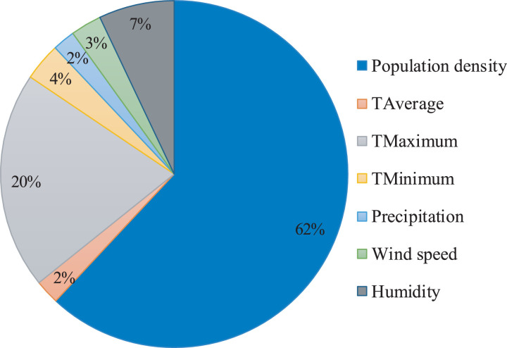
In order to obtain the relative importance of each input variable, a parametric study was performed. In this regard, the change in the infection rate was measured when a variable was altered from its lowest to highest values, and other variables were fixed on their average values. By calculating the changes in the infection rate for all input variables, their values were normalized and expressed in percentage to obtain their relative importance. Fig. 8 illustrates the relative importance of all input variables using the ANFIS-VOA-II model. As revealed in this figure, the population density with the relative importance of 62% is by far the most critical variable. The maximum temperature with the relative importance of almost one-third of the population density is in the second rank, and the humidity variable with the relative importance of about one-ninth of the population density has the third rank. The other five climatology variables have the relative importance of less than 10% so that the sum of their relative importance is still 2% less than the relative importance of the maximum temperature, and it is also about 30% of the relative importance of the population density. Moreover, the precipitation and the average temperature are the two climatology variables held in the lowest rank.
Fig. 8.
The relative importance of the climatology variables on the infection rate.
The changing trends of the infection rate by changing the input variables are shown in Fig. 9 . By increasing the population density, the infection rate grows significantly, which can be a sign of the importance of social distancing. It can also be seen that as the average and maximum temperature of weather increase, the infection rate decreases, but the reduction is more in the case of the maximum temperature. Additionally, the slight decline in the infection rate is observed by increasing the wind speed. Moreover, with increasing the humidity of the county, the infection rate rises.
Fig. 9.
The change trend of the infection rate by changing the climatology variables.
5. Summary and concluding remarks
The rapid spread of the novel Coronavirus disease (i.e., COVID-19) has become a serious global issue. The official statistics shows that the U.S. is on top of the list of confirmed infected cases by the COVID-19. Previous studies have shown that several factors could potentially affect the spread and transmission rates of the viruses including population density and climatology parameters. In this study, a combination of the virus optimization algorithm (VOA) and adaptive network-based fuzzy inference system (ANFIS) was used to investigate the effects of various climate-related factors and population density on the spread of the COVID-19. The use of the VOA can optimize the centers and spreads of membership functions of input variables as well as the regression coefficients of the consequence parts of fuzzy rules in such a way to avoid the local optima. To develop the predictive models, a dataset containing information on the climate related factors (i.e., average temperature, maximum temperature, minimum temperature, precipitation, average annual humidity, and average annual wind speed) and population density were used as input variables while infection rate was defined as the only output variable.
The developed models based on the machine learning technique could successfully predict the effects of the different variables on the infection rate and showed superior performance compared to the linear regression. Among the input variables, population density showed the most significant effect on the infection rate. This finding highlights the importance of social distancing in reducing the infection rate. Among the climate parameters, maximum temperature was found to have the most significant effect on the infection rate. An increase in the maximum temperature could reduce the infection rate. Average temperature, minimum temperature, precipitation, and average wind speed were not found to significantly affect the spread of the COVID-19 while an increase in the relative humidity was found to slightly increase the infection rate. The findings of this research show that it could be expected to have slightly reduced infection rate over the summer season. However, it should be noted that the models developed in this study were based on limited one-month data. Future investigation can benefit from using more comprehensive data covering a wider range for the input variables.
CRediT authorship contribution statement
Ali Behnood: Conceptualization, Data curation, Validation, Writing - original draft, Writing - review & editing. Emadaldin Mohammadi Golafshani: Conceptualization, Software, Methodology, Writing - original draft, Writing - review & editing. Seyedeh Mohaddeseh Hosseini: Data curation, Writing - original draft.
Declaration of Competing Interest
The authors declare that they have no known competing financial interests or personal relationships that could have appeared to influence the work reported in this paper.
References
- 1.Lahmiri S, Bekiros S. The impact of COVID-19 pandemic upon stability and sequential irregularity of equity and cryptocurrency markets. Chaos, Solitons & Fractals. 2020;138 doi: 10.1016/j.chaos.2020.109936. doi: [DOI] [PMC free article] [PubMed] [Google Scholar]
- 2.Sun T, Wang Y.Modeling COVID-19 epidemic in Heilongjiang Province, China. Chaos, Solitons & Fractals2020:109949. doi: 10.1016/j.chaos.2020.109949. [DOI] [PMC free article] [PubMed]
- 3.Arias Velásquez RM, Mejía Lara JV. Forecast and evaluation of COVID-19 spreading in USA with reduced-space Gaussian process regression. Chaos, Solitons & Fractals. 2020;136 doi: 10.1016/j.chaos.2020.109924. doi: [DOI] [PMC free article] [PubMed] [Google Scholar]
- 4.Ribeiro MHDM, da Silva RG, Mariani VC, Coelho L dos S. Short-term forecasting COVID-19 cumulative confirmed cases: perspectives for Brazil. Chaos, Solitons & Fractals. 2020;135 doi: 10.1016/j.chaos.2020.109853. doi: [DOI] [PMC free article] [PubMed] [Google Scholar]
- 5.Wang J, Tang K, Feng K, Lv W. High temperature and high humidity reduce the transmission of COVID-192020.
- 6.Ahmadi M, Sharifi A, Dorosti S, Ghoushchi SJ, Ghanbari N. Investigation of effective climatology parameters on COVID-19 outbreak in Iran. Sci Total Environ. 2020;729 doi: 10.1016/j.scitotenv.2020.138705. doi: [DOI] [PMC free article] [PubMed] [Google Scholar]
- 7.Pirouz B, Shaffiee Haghshenas S, Pirouz B, Shaffiee Haghshenas S, Piro P. Development of an assessment method for investigating the impact of climate and urban parameters in confirmed cases of COVID-19: A new challenge in sustainable development. Int J Environ Res Public Health. 2020;17 doi: 10.3390/ijerph17082801. [DOI] [PMC free article] [PubMed] [Google Scholar]
- 8.Pirouz B, Shaffiee Haghshenas S, Shaffiee Haghshenas S, Piro P. Investigating a serious challenge in the sustainable development process: analysis of confirmed cases of COVID-19 (new type of coronavirus) through a binary classification using artificial intelligence and regression analysis. Sustainability. 2020;12 doi: 10.3390/su12062427. [DOI] [Google Scholar]
- 9.Geoghegan JL, Holmes EC. Predicting virus emergence amid evolutionary noise. Open Biol. 2017;7 doi: 10.1098/rsob.170189. [DOI] [PMC free article] [PubMed] [Google Scholar]
- 10.Xie J, Zhu Y. Association between ambient temperature and COVID-19 infection in 122 cities from China. Sci Total Environ. 2020;724 doi: 10.1016/j.scitotenv.2020.138201. [DOI] [PMC free article] [PubMed] [Google Scholar]
- 11.Lowen AC, Mubareka S, Steel J, Palese P. Influenza virus transmission is dependent on relative humidity and temperature. PLOS Pathog. 2007;3:e151. doi: 10.1371/journal.ppat.0030151. [DOI] [PMC free article] [PubMed] [Google Scholar]
- 12.Altamimi A, Ahmed AE. Climate factors and incidence of Middle East respiratory syndrome coronavirus. J Infect Public Health. 2019 doi: 10.1016/j.jiph.2019.11.011. [DOI] [PMC free article] [PubMed] [Google Scholar]
- 13.Kandiri A, Mohammadi Golafshani E, Behnood A. Estimation of the compressive strength of concretes containing ground granulated blast furnace slag using hybridized multi-objective ANN and salp swarm algorithm. Constr Build Mater. 2020;248 doi: 10.1016/j.conbuildmat.2020.118676. [DOI] [Google Scholar]
- 14.Behnood A, Golafshani EM. Machine learning study of the mechanical properties of concretes containing waste foundry sand. Constr Build Mater. 2020;243 doi: 10.1016/j.conbuildmat.2020.118152. [DOI] [Google Scholar]
- 15.Daneshvar D, Behnood A.Estimation of the dynamic modulus of asphalt concretes using random forests algorithm. Int J Pavement Eng 2020:1–11. doi: 10.1080/10298436.2020.1741587. [DOI]
- 16.Rivers-Moore NA, Hill TR. A predictive management tool for blackfly outbreaks on the Orange River, South Africa. River Res Appl. 2018;34:1197–1207. doi: 10.1002/rra.3357. [DOI] [Google Scholar]
- 17.Yin R, Tran VH, Zhou X, Zheng J, Kwoh CK. Predicting antigenic variants of H1N1 influenza virus based on epidemics and pandemics using a stacking model. PLoS One. 2018;13 doi: 10.1371/journal.pone.0207777. [DOI] [PMC free article] [PubMed] [Google Scholar]
- 18.Agarwal N, Koti SR, Saran S, Kumar AS. Data mining techniques for predicting dengue outbreak in geospatial domain using weather parameters for New Delhi, India. Curr Sci. 2018;114:2281–2291. [Google Scholar]
- 19.Anno S, Hara T, Kai H, Lee M-A, Chang Y, Oyoshi K, et al. Spatiotemporal dengue fever hotspots associated with climatic factors in Taiwan including outbreak predictions based on machine-learning. Geospat Health. 2019;14:183–194. doi: 10.4081/gh.2019.771. [DOI] [PubMed] [Google Scholar]
- 20.Chenar SS, Deng Z. Development of artificial intelligence approach to forecasting oyster norovirus outbreaks along Gulf of Mexico coast. Environ Int. 2018;111:212–223. doi: 10.1016/j.envint.2017.11.032. [DOI] [PubMed] [Google Scholar]
- 21.Chenar SS, Deng Z. Development of genetic programming-based model for predicting oyster norovirus outbreak risks. Water Res. 2018;128:20–37. doi: 10.1016/j.watres.2017.10.032. [DOI] [PubMed] [Google Scholar]
- 22.Shamkhali Chenar S, Deng Z. Environmental indicators of oyster norovirus outbreaks in coastal waters. Mar Environ Res. 2017;130:275–281. doi: 10.1016/j.marenvres.2017.08.009. [DOI] [PubMed] [Google Scholar]
- 23.Jiao W, Zhiqiang D. Modeling and prediction of oyster norovirus outbreaks along Gulf of Mexico Coast. Environ Health Perspect. 2016;124:627–633. doi: 10.1289/ehp.1509764. [DOI] [PMC free article] [PubMed] [Google Scholar]
- 24.Liang R, Lu Y, Qu X, Su Q, Li C, Xia S, et al. Prediction for global African swine fever outbreaks based on a combination of random forest algorithms and meteorological data. Transbound Emerg Dis. 2020;67:935–946. doi: 10.1111/tbed.13424. [DOI] [PubMed] [Google Scholar]
- 25.Topak L, Hamidi O, Fathian M, Karami M. Comparative evaluation of time series models for predicting influenza outbreaks: application of influenza-like illness data from sentinel sites of healthcare centers in Iran. BMC Res Notes. 2019;12:353. doi: 10.1186/s13104-019-4393-y. [DOI] [PMC free article] [PubMed] [Google Scholar]
- 26.Salgotra R, Gandomi M, Gandomi AH. Time Series Analysis and forecast of the COVID-19 pandemic in India using genetic programming. Chaos, Solitons & Fractals. 2020 doi: 10.1016/j.chaos.2020.109945. [DOI] [PMC free article] [PubMed] [Google Scholar]
- 27.USAFacts. Coronavirus locations: COVID-19 map by county and state2020. https://usafacts.org/visualizations/coronavirus-covid-19-spread-map/(accessed April 28, 2020).
- 28.NOAA. Climate at a Glance - (National Center for Environmental Information)2020. https://www.ncdc.noaa.gov/cag/county/mapping(accessed April 28, 2020).
- 29.USA.com. Your local guide to cities, towns, neighborhoods, states, counties, metro areas, zip codes, area codes, and schools in USA2020. http://www.usa.com/(accessed April 28, 2020).
- 30.Liang Y-C, Cuevas Juarez JR. A novel metaheuristic for continuous optimization problems: virus optimization algorithm. Eng Optim. 2016;48:73–93. doi: 10.1080/0305215X.2014.994868. [DOI] [Google Scholar]
- 31.Jang JSR. ANFIS: adaptive-network-based fuzzy inference system. IEEE Trans Syst Man Cybern. 1993;23:665–685. doi: 10.1109/21.256541. [DOI] [Google Scholar]
- 32.Takagi T, Sugeno M. Fuzzy identification of systems and its applications to modeling and control. IEEE Trans Syst Man Cybern. 1985;SMC-15:116–132. [Google Scholar]
- 33.Chiu SL. Fuzzy model identification based on cluster estimation. J Intell Fuzzy Syst. 1994;2:257–278. doi: 10.3233/IFS-1994-2306. [DOI] [Google Scholar]
- 34.Peizhuang W. Pattern recognition with fuzzy objective function algorithms (James C. Bezdek) SIAM Rev. 1983 doi: 10.1137/1025116. [DOI] [Google Scholar]
- 35.Golafshani EM, Behnood A, Arashpour M. Predicting the compressive strength of normal and High-Performance Concretes using ANN and ANFIS hybridized with Grey Wolf Optimizer. Constr Build Mater. 2020;232 doi: 10.1016/j.conbuildmat.2019.117266. [DOI] [Google Scholar]


