Abstract
Calculating the cup-to-disc ratio is one of the methods for glaucoma screening with other clinical features. In this paper, we propose a graph convolutional network (GCN) based method to implement the optic disc (OD) and optic cup (OC) segmentation task. We first present a multi-scale convolutional neural network (CNN) as the feature map extractor to generate feature map. The GCN takes the feature map concatenated with the graph nodes as the input for segmentation task. The experimental results on the REFUGE dataset show that the Jaccard index (Jacc) of the proposed method on OD and OC are 95.64% and 91.60%, respectively, while the Dice similarity coefficients (DSC) are 97.76% and 95.58%, respectively. The proposed method outperforms the state-of-the-art methods on the REFUGE leaderboard. We also evaluate the proposed method on the Drishthi-GS1 dataset. The results show that the proposed method outperforms the state-of-the-art methods.
1. Introduction
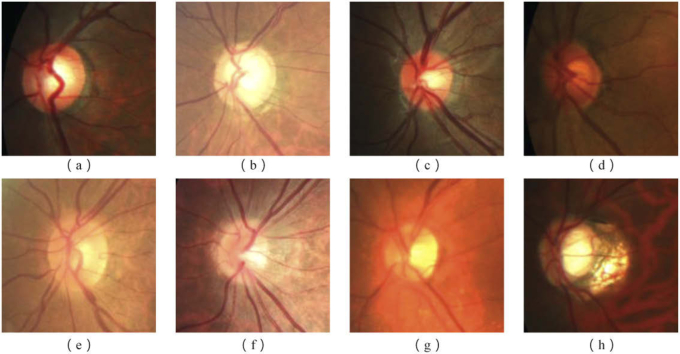
Retinal image analysis has a wide range of clinical applications, such as the screening of glaucoma. Glaucoma is a chronic and irreversible eye disease, which is currently the leading cause of global irreversible blindness [1]. It is characterized by structural changes in the optic nerve head, which occurs preferentially at the superior and inferior poles of the optic disc (OD) [2]. In addition, the optic cup (OC) enlarges vertically more than horizontally. Therefore, a large vertical cup-to-disc ratio (vCDR) is considered as a distinctive feature of glaucoma, and the measurement of vCDR has a clinical significance for structural screening and diagnosis. Glaucoma symptoms include the changes in retinal nerve fiber layer and/or optic nerve head, such as the thinning of neuro retinal rim and the growing of optic cup, resulting in an increased vCDR. The measurement of vCDR combined with other clinical features is one of the methods used to classify glaucoma [1,3]. Manual labeling is a time-consuming and tedious task. Therefore, an automatic segmentation method is urgently needed. In clinical practice, color fundus photography is the most cost-effective imaging modality for the examination of retinal disorders [4]. In color fundus images, OD and OC usually appear as bright yellow regions. Examples of fundus images from a normal eye and glaucoma are shown in Fig. 1. Due to the variations in shape, size, and color of OD and OC regions, it is a challenging task to get a reliable and accurate segmentation result of OD and OC in color fundus images. OD may have notable difference in color, and the border between the OD and OC may be blurred. This situation also exists between OD and other area. Several challenging examples of color fundus images with different appearance are shown in Fig. 2.
Fig. 1.
Examples of (a) normal and (b) glaucoma fundus images from REFUGE [4] dataset. The right-hand image of each example contains enlarged optic disc area, where optic disc and cup are indicated by outer blue and inner green lines, respectively. The vertical lines indicate the diameter of the optic disc and cup. Note that the eye with glaucoma has a much larger cup-to-disc ratio than the normal eye.
Fig. 2.
Examples of optic disc (OD) and optic cup (OC) appearance from REFUGE [4] dataset. The first row shows different colors of optic disc, which are (a) Yellowish OD, (b) Whitish OD, (c) Reddish OD, (d) Brownish OD. The second row shows several challenging examples, which are (e) obscure border between optic disc and cup, (f, g) blurred border between optic disc and other area and (h) structure change of OD.
A lot of efforts have been made in the recent years from the medical imaging community to develop automated methods for OD and OC segmentation, which augments the recognition quality and reduces prediction time. According to the working principle, existing methods for OD and OC segmentation are mainly divided into three categories, which are template matching, deformable models and machine learning based method [5–8].
For template-based methods, Aquino et al. [9] and Cheng et al. [10] modeled the OD as a circle and an ellipse, respectively. They utilized edge detection techniques followed by a Hough transform to detect the edges in the image. Another form of this approach is the Hausdorff-based template matching, which was proposed by Lalonde et al. [11]. Their method relies on Hausdorff-based template matching guided by a pyramidal decomposition for object tracking. Wong et al. [12] proposed a modified version of the conventional level-set approach to obtain the OD boundary, which is smoothed by fitting an ellipse. Zheng et al. [13] integrated a prior information with the OC and OD. The segmentation task was performed by using a general energy function based on graph cut technique. Template based methods are easy to implement, but may require a lot of sampling points and with limited robustness.
Deformable model-based methods need an initial contour for initialization and then deform toward the target edge according to various energy terms, which are usually defined by using image gradient, image intensity and boundary smoothness [14]. Osareh et al. [15] and Lowell et al. [16] determined the OD center location firstly. Then, the OD boundary can be extracted by a deformable contour. Xu et al. [17] labeled the contour points as positive or uncertain points after each snake deformation, which is used to refine the OD boundary before the next contour deformation. Joshi et al. [18] improved the Chan-Vese model by using two texture feature spaces near the analyzed pixels and local red channel intensities. A modified region-based active contour model was used to segment OD boundary. Deformable model-based methods could acquire desirable results, but they are usually sensitive to the initialization.
Recently, machine learning-based method has been demonstrated to be a powerful tool in segmentation task [19–22]. This method trains a classifier from existing labeled image data and predicts N probabilities for each pixel in the image domain, where N is the number of classes. Therefore, a category of each pixel can be obtained from the predicted probabilities. For OD and OC segmentation and analysis, Fu et al. [23] employed an U-shape multi-label convolutional network (M-Net) for joint OD and OC segmentation, which is combined with an input layer and a side-output layer. Maninis et al. [24] performed OD segmentation by using Fully-convolutional neural network [19] based on a VGG-16 net [25] and a transfer learning technique. Most of the machine learning-based methods described above can automatically segment OD and OC, and obtain desired segmentation result. However, they are pixel-wise segmentation methods that require more computation resources. In this respect, the graph convolutional network (GCN) can reduce the computation consumption by only predicting the object contour. As far as we know, no GCN-based method has been proposed for OD and OC segmentation. Ling et al. [26] proposed to predict all vertices of object contour based on GCN. However, they ignored the multi-scale feature, which limits the extraction capability of the representative feature and restricts the segmentation performance.
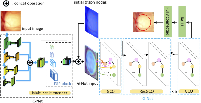
In this paper, to overcome the aforementioned problems, we propose a graph convolutional network (GCN) based method for the OD and OC segmentation. The proposed method includes two main parts, as illustrated in Fig. 3. The first part is a multi-scale convolutional neural network called C-Net, which is used to generate the feature map of the input images. Many traditional deep convolutional neural networks (DCNN) ignore the multi-scale feature, which limits the representative feature extraction capability. The second part of the proposed method is a graph convolutional network, called G-Net. The input of the G-Net is the multi-scale feature map from C-Net, concatenated with the initial graph nodes/vertices. In our proposed segmentation method, we take the segmentation task as a regression problem. The boundary contour of the OD or OC is presented as a graph, which contains N vertices. The locations of all vertices are predicted simultaneously by the G-Net.
Fig. 3.
Overview of the proposed method. C-Net, a multi-scale convolutional neural network, outputs the feature map of the input images. G-Net, a graph convolutional network, takes the output of C-Net and the initial graph nodes as input. The output of a fully connected layer following the G-Net is our final segmentation result.
The rest of paper is organized as follows. The details of the proposed method are described in Section 2. Section 3 shows the experimental results, including the data description, evaluation results of the proposed method and comparison with other segmentation methods. Finally, a discussion is provided with conclusion in Section 4.
2. Methods
2.1. Overview of the proposed method
The proposed method includes two main parts, as shown in Fig. 3. The first part called C-Net is a multi-scale convolutional neural network, which is used to generate the feature maps of the input images. The second part called G-Net is a graph convolutional network, which is used to predict the vertices of the OD or OC contour.
In our C-Net, a modified ResNet [27] is used as the backbone network. We concatenate the low level features such as corners and edges of the input image, as well as the high level semantic features in the deep layers of the network at same time. The concatenated feature is input to a pyramid scene parsing (PSP) block [21] that is used to obtain multi-scale features. The output of the PSP block and the initial graph nodes are concatenated as the input of the G-Net. Our G-Net is a graph convolutional network with six residual graph convolutional operations (ResGCOs) and two graph convolutional operations (GCOs). Finally, a fully connected layer with ReLU [28] activation function is used as our final output layer. In this paper, the proposed network is trained based on a contour matching loss function.
2.2. Convolutional neural network (C-Net)
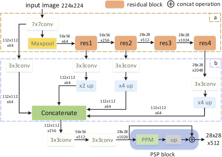
Our convolutional neural network is a modified ResNet-101, which is used as the feature extractor of the input images. Deep network architecture and repeated down-sampling operation in many CNNs make it difficult to obtain effective features in the last layer for object representation. Motivated by U-Net [20] architecture, we proposed a multi-scale convolutional neural network called C-Net, which is shown in Fig. 4. Resnet-101 is used as the main structure of C-Net (Fig. 4. Part a), but the last average pooling layer and the fully connected layer of ResNet-101 are removed. Meanwhile, the dilation convolution operation with 2 and 4 dilated rates are used in the last two residual blocks (Fig. 4. res3 and res4), respectively. In this residual structure, only the 7 7 convolution is followed by a maxpooling operation. The feature maps in the residual blocks are down-sampled by convolution operation with a stride of 2. In order to obtain multi-scale features of the input image, we use four 3 3 convolution operations to encode features obtained from the convolution, residual block 1, 2, 4, respectively (Fig. 4. Part b). To concatenate features obtained from the convolution operations, bilinear up-sampling operations with 2 and 4 scale factors are added to make these feature maps have the same spatial size of . The concatenated feature passes through two convolution operations and are feed into the PSP block to obtain C-Net output feature with a dimension of . The pyramid parsing module (PPM) [21] was used to extract multiscale features. In addition, the convolution and each convolution operation in the C-Net are also followed by a batch normalization operation and a ReLU activation function. The input of PSP block is the output of two cascaded convolution operations in C-Net.
Fig. 4.
C-Net architecture. In the figure, conv and conv represent and convolution operation, respectively, while up and up represent bilinear up-sampling operation with 2 and 4 scale factors, respectively. The numbers on the arrows represent the sizes of feature maps. The pyramid parsing module (PPM) [21] was used to extract multi-scale features.
2.3. Graph-based convolutional neural network (G-Net)
In this section, the theoretical motivation for a graph-based convolutional neural network model is introduced. A graph is used in Graph Convolutional Network [29], where and are the set of nodes and edges respectively. The layer-wise propagation rule of a multi-layer GCN can be formulated as:
| (1) |
where is the adjacent matrix of an undirected graph with self-connections. is the identity matrix. is a trainable weight of the GCN layer. is an activation function. is a matrix of activations in the GCN layer, where is the number of nodes and is the dimension of the input feature. is the output feature of layer, where is the dimension of the output feature.
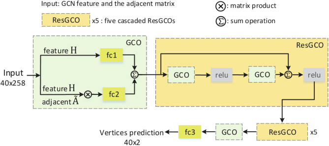
To get the initial graph, we firstly localize the disc region by using the existing detection method [23], and then crop the fundus image based on the detected disc region. We initialize nodes along a circle centered in the cropped image with a diameter of image height for the optic disc and a diameter of 70% of image height for the optic cup. In the G-Net, the segmentation task is considered as a regression problem. The boundaries of OD and OC are presented as a graph, which contains N vertices. G-Net is trained to predict the shift of the nodes from the initial locations to their ground truth locations. In order to obtain effective shift information, two GCOs and six cascaded ResGCOs are proposed. The GCO contains a matrix product operation and two fully connected layers, which is used to adjust the feature dimension. The ResGCO is constructed by two GCOs with a short skip connection, which is used to learn the representative feature. Finally, we apply a single fully connected layer to the output feature of the G-Net and predict a relative shift of each vertex from the initial location to the ground truth location. For each vertex, the new location of will be updated to after a graph convolutional operation. G-Net architecture is shown in Fig. 5. In our implementation, the G-Net is executed times and the final step is used as the final result. T is an empirical value that was set as 3 in the experiment. The contour matching loss is used to monitor the training process of G-Net.
Fig. 5.
G-Net architecture. The graph convolution operation (GCO) is used at the beginning and end of the G-Net to adjust the feature dimension. The residual graph convolution operation (ResGCO) is used to learn more representative feature for segmentation.
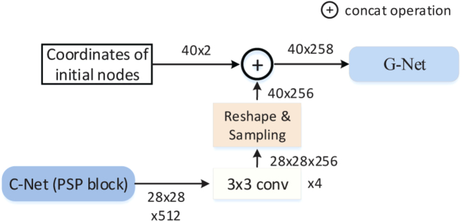
In the experiment, we use 40 points as nodes of the graph. Each node takes one pixel in the contour. The neighboring nodes are connected with spline curves to form a smooth contour. Two initial contours were used to segment OD and OC, respectively. The convnet features (C-Net output) are linked with the nodes based on the concatenation operation. The concatenation operation can assign the convnet feature to the nodes as a feature vector. Figure 6 shows how the convnet feature linked with the nodes to form G-Net input features (). The G-Net input features will be updated by the GCN. The updated features are then used to predict the new locations of the nodes.
Fig. 6.
The connection of the C-Net and G-Net. It shows how the C-Net feature linked with the nodes.
2.4. Loss function
In this paper, a contour matching loss is presented to evaluate the difference between the ground truth contour and the predicted contour of the OD and OC. In order to make a precise matching between the ground truth contour and the predicted contour, the ground truth and the predicted contour vertices are assumed have a same well-defined order. The contour vertices of the ground truth are defined as , and the predicted vertices are defined as . The contour vertices matching loss can be formulated as follows.
| (2) |
where is the number of the contour vertices, and are the indexes of the ordered vertices of the ground truth contour and the prediction, respectively.
3. Results
3.1. Materials
Public fundus image dataset REFUGE [4] for OD and OC segmentation was employed to evaluate the performance of the proposed method. The dataset consists of 1200 color fundus images, 120 with glaucoma and 1080 without. All fundus images are stored in JPEG format, with 8 bits per color channel. The dataset was divided into three subsets officially, each of them contains 400 fundus images and has equal proportion of glaucomatous (10%) and non-glaucomatous (90%) cases. The fundus images were acquired by two devices: a Zeiss Visucam 500 fundus camera with a resolution of pixels and a Canon CR-2 device with a resolution of pixels. Specifically, one subset was acquired from Zeiss Visucam 500 camera, while other two subsets were acquired from Canon CR-2 device. The annotation of OD and OC in each image was manually labeled by experts. The ground-truth of REFUGE test set is publicly available.
The Drishti-GS1 [30,31] dataset was used to evaluate the robustness of the model. The dataset contains 101 images that were collected at Aravind eye hospital, Madurai, India. All images were labelled by 4 eye experts with different clinical experiences. In this dataset, 50 images were selected as training set, while 51 images were selected as test set.
3.2. Evaluation metrics and experiment design
Different quantitative metrics were employed to evaluate the performance of the proposed method, which are Dice similarity coefficient (DSC), Jaccard index (Jacc), also called intersection over union (IoU), Sensitivity (Sen.), and Specificity (Spec.) for OD and OC separately, and the mean absolute error (MAE) of the vCDR estimations. In particular, most of the existing works for OD and OC segmentation were evaluated according to Jacc. Therefore, Jacc was selected as a main metric for comparison between different methods.
The Jacc index and DSC measure the overlap between two regions, which are defined as:
| (3) |
where and are the ground truth and predicted segmentations of the region of interest k, respectively (with k = OD or OC).
The MAE is defined as:
| (4) |
where is a function that estimates the vCDR based on the vertical diameter of the segmentations of the OD and the OC, respectively.
The Sen. and Spec. are defined as:
| (5) |
where TP, TN, FP, and FN present true positive, true negative, false positive, and false negative, respectively.
3.3. Training details and parameter setting
The proposed method was mainly implemented by a deep learning framework PyTorch and Python language. The implementation code of the method ran on a platform of Ubuntu 16.04 with 1 GPU of NVIDIA GTX 1070. The implementation code was not optimized and did not use multi-thread and parallel programming.
In the C-Net and G-Net, all convolutions are followed by a batch normalization. The number of epochs was 27. Adam optimizer was used to train the model and the training batch size was 6. For other hyperparameters, the initial learning rate is 3e-4, weight decay is 1e-5 and the initial learning rate was decayed by gamma=0.1 every 4 epochs.
3.4. Experimental results
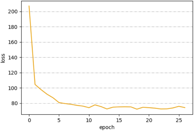
The loss curve of the training process is shown in Fig. 7. With the contour matching loss function, the loss value decreases smoothly. It also shows that the training hyperparameters were set properly.
Fig. 7.
The loss curve of the training process. The number of epochs was 27.
Table 1 shows the quantitative results of the proposed method on REFUGE test set. Table 2 shows the comparison of the proposed method with the state-of-the-art segmentation methods on the REFUGE leaderboard. Ranked first and second methods were chosen for comparison. The bold font represents the best performance. Figure 8 shows the receiver operating characteristics (ROC) curve of our classification result for glaucoma/normal derived from the calculated vCDR. We only used vCDR for glaucoma classification without any additional processing. A higher vCDR value represents a higher risk of glaucoma. The ROC curve is created by plotting the true positive rate (TPR) against the false positive rate (FPR) at various threshold settings. From the Fig. 8, we can observe that the calculation of the vCDR derived from the segmentations performs similarly to the one derived from the ground truth segmentation, in terms of AUC to predict glaucoma.
Table 1. Quantitative results of the proposed method on REFUGE test set. Avg., Std., Max and Min represent average values, standard deviations, maximum and minimum, respectively.
| Jacc (%) | DSC (%) | Sen. (%) | Spec. (%) | ||
|---|---|---|---|---|---|
| DISC | Avg. | ||||
| Std. | |||||
| Max | |||||
| Min | |||||
|
| |||||
| CUP | Avg. | ||||
| Std. | |||||
| Max | |||||
| Min | |||||
Table 2. Comparison with the state-of-the-art methods. Dice similarity coefficients (DSC) metric was used for evaluating the optic cup and disc, while the mean absolute error (MAE) was used for evaluating the vertical cup-to-disc ratio (vCDR).
| Method | Disc rank | Cup rank | vCDR MAE rank | Disc DSC(%) | Cup DSC(%) | MAE |
|---|---|---|---|---|---|---|
| CUHKMED | 1 | 2 | 2 | 96.02 | 88.26 | 0.0450 |
| Masker | 7 | 1 | 1 | 94.64 | 88.37 | 0.0414 |
| Ours | - | - | - | 97.76 | 95.58 | 0.0136 |
Fig. 8.
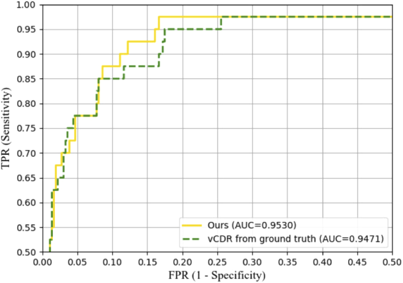
The receiver operating characteristics (ROC) curves and the area under the curve (AUC) values of the proposed method and the ground truth on REFUGE test set.
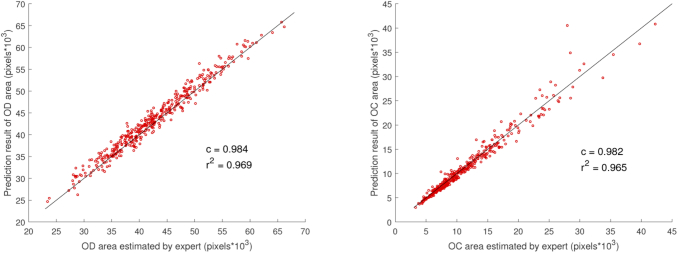
Correlation analysis was performed to assess the reliability of the proposed method. Figure 9 shows the scatter plot of the predicted area (total number of pixels) using proposed method vs. the expert manually labeled area. High correlation coefficient demonstrates that the proposed method gives a satisfactory segmentation result. High determination coefficient means that most points are near to the line, which shows no systematic difference.
Fig. 9.
Correlation analysis of the segmentation results with ground-truth for (a) optic disc (OD) and (b) optic cup (OC), which uses area as the evaluation standard. The black line indicates no systematic difference. and represent correlation coefficient and determination coefficient, respectively.
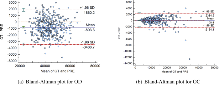
The area deviations of OD and OC are shown in the Bland-Altman plot (Fig. 10), which measures the agreement between the manually labeled region and the region obtained from the proposed method. Two red dotted lines indicate the average 1.96 standard deviation, and the interval formed by the red lines indicates the 95% limits of agreement (LoA). The two sets of data are consistent when the most of scattered points fall within the 95% LoA. 23 points fall outside of the 95% LoA for OD, and 17 for OC. The blue solid and orange dotted line indicate the mean value of the differences and zero bias line, respectively. The closer the blue line with the orange line, the better the segmentation performance. It can be observed that most cases fall within the 95% LoA and the average of the OC segmentation difference is very close to 0.
Fig. 10.
Bland-Altman plot of the agreement between the manually labeled regions and the segmentation results obtained from the proposed method for (a) optic disc (OD) and (b) optic cup (OC). Area was used as the evaluation standard. The horizontal and vertical axis represent the average value and the difference of the predicted (PRE) area and the manually labelled (i.e. ground-truth (GT)) area, respectively.
Table 3 shows the comparison of the proposed method with CNN methods [19–22] on REFUGE test set. We used the official implementations code for all the experiments, and the parameters were established by authors. The evaluation results were reported as average standard deviation. It can be observed that the proposed method achieves the highest Jacc with the lowest standard deviation. Moreover, the segmentation performance of the proposed method on OD and OC is superior to other methods. The testing for statistical significance was performed at the OD and OC between the reference methods and our method in terms of Spec., Jacc and DSC. The analysis shows that there is a statistically significant difference at the OD and OC in terms of the three metrics. Significance analysis demonstrates the superiority of the GCN based method. For segmentation of OD, PSPNet tends to be over-segmentation. Therefore, its sensitivity is higher than ours. However, its specificity is lower than ours. For segmentation of OC, the sensitivity of FCN is higher than ours, but its variance is larger and the specificity is lower than ours.
Table 3. Comparison with other segmentation methods on REFUGE test set. Our method achieves the highest Jacc with the lowest standard deviation.
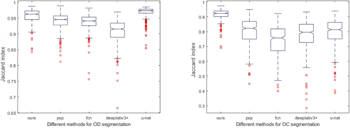
Figure 11 shows the box plots, which indicates the distribution of the Jacc from the different methods. It can be observed that the proposed method has the highest median Jacc and the lowest deviation.
Fig. 11.
Jacc distribution of different segmentation methods on optic disc (OD) and optic cup (OC). The box plot is composed of 5 metrics, which are minimum value, lower quartile, median, upper quartile, and maximum value. The red points represent outliers.
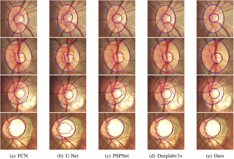
Figure 12 shows several segmentation results of OD and OC with different appearance situations, where red and blue lines indicate the segmentation results and manually labeled results. It can be observed that the existence of blurred border confuses the other methods and causes erroneous segmentation results. In contrast, the proposed method works well for most cases in the given examples and the segmentation results are relatively accurate.
Fig. 12.
Result visualization of optic disc (OD) and optic cup (OC) segmentation, where blue curves are manually labelled by expert and red curves are predictions of the methods. The first to fourth rows show the different appearance of OD and OC, including boundary blurring between OD and OC (the first row), blurring between OD and external area (the second row) and structural changes of OD and OC (third and fourth row). Each column represents a segmentation method, which is FCN, U-Net, PSPNet, Deeplabv3+ and the proposed method, respectively.
To verify the robustness of the proposed method on normal and glaucoma images, we evaluated the segmentation results of these two categories respectively. The evaluation results are shown in Table 4. From the table, we can see that the segmentation accuracies of glaucoma and normal images are close. In addition, we trained the model on REFUGE dataset and tested it on Drishti-GS1 test set. The results were compared with several state-of-the-art methods, which are shown in Table 5. DSC values of these methods were obtained from their corresponding papers. From the table, we can observe that the model trained on the REFUGE training set can predict the images in the Drishti-GS1 test set with satisfactory accuracies. Therefore, the model is robust between different datasets.
Table 4. The segmentation result of the proposed method for glaucoma and normal images on the REUFGE test set.
| Glaucoma |
Normal |
|||
|---|---|---|---|---|
| Cup | Disc | Cup | Disc | |
| Jacc(%) | ||||
| DSC(%) | ||||
| Sen.(%) | ||||
| Spec.(%) | ||||
Table 5. Comparison with other state-of-the-art methods on Drishti-GS1 test set.
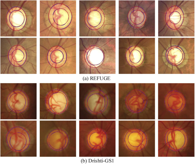
Figure 13 shows the segmentation results of glaucoma on two test sets. It can be observed that the model can handle the irregular shape and the blurred border cases. Figure 14 shows a limitation of the proposed method. Figure 14(a) and (b) show two cases with the inferior segmentation results on the optic cup, where (a) has the limited Jacc and specificity and (b) has the limited sensitivity in the test set. Figure 14(c)-(f) show the cases with the inferior segmentation results on the optic disc, which have the limited performance on Jacc, sensitivity or specificity in the test set.
Fig. 13.
Segmentation results of the proposed method for glaucoma cases in (a) REFUGE test set and (b) Drishti-GS1 test set, respectively.
Fig. 14.
The limitations of the proposed method. These images have blurred target edges and irregular border shape.
4. Discussion and conclusion
In this work, we propose a graph convolutional network based method for the automatic segmentation of optic disc and cup region in fundus images. The two key parts of the proposed network are G-Net and C-Net. In order to acquire rich feature information, we employ a multi-scale convolutional neural network (C-Net) as the feature extractor, which learns the low-level and high-level features to assist G-Net for further prediction. The output feature of C-Net is concatenated with the graph nodes as input of G-Net for the subsequent prediction.
We performed a series of experiments to verify the effectiveness and the advantage of the proposed method compared with other segmentation methods. Compared with other reference methods, the proposed method performs best, which gets a mean Jacc of 95.64% and 91.60% for optic disc and cup, respectively. In addition, the significance analysis demonstrates the superiority of the proposed method. We also evaluated the robustness of the proposed method by testing on normal and glaucoma images, respectively. To verify that the model can work well on different datasets, we trained the model on REFUGE dataset and tested it on Drishti-GS1 test set. The results showed that the proposed method is robust between different datasets. From Fig. 8, we can observe that the proposed method obtains an AUC of 0.9530 for glaucoma classification. The result is inferior to that of CUHKMED (AUC=0.9644) [4]. The reason is that we only used vCDR for the glaucoma classification without any additional processing. However, CUHKMED use a pre-processing for glaucoma classification. Specifically, CUHKMED used two ellipses to fit the OD and OC masks to obtain vCDR. In addition, they normalized vCDR into 0-1 as a final segmentation classification probability.
From the visualization of the segmentation results, it can be observed that blurring bounders and structural changes in disc/cup are the main challenges, which may result in segmentation failure by other methods. However, the proposed method can handle these conditions and give more reliable results for both normal and glaucoma cases. For further evaluation, the sensitivity and specificity of the optic disc and cup segmentation were also calculated. The mean sensitivity of optic disc and cup are 98.73% and 94.93%, while the specificity are 99.95% and 99.99%, respectively. We also analyzed the cases with decreased segmentation accuracies. The main reasons are the structural changes and irregular edges of the optic disc/cup. Our future work will focus on developing robust and accurate methods.
In summary, we propose an image segmentation method based on GCN. The proposed method outperforms several state-of-the-art methods on the REFUGE dataset and Drishthi-GS1 dataset. In our subsequent studies, we will study the problem of learning irregular edges by increasing the number of GCN vertices. In addition, we have intentions to apply the proposed method for more organ segmentation tasks.
Funding
National Natural Science Foundation of China10.13039/501100001809 (61876148, 61971343).
Disclosures
The authors declare no conflicts of interest.
References
- 1.Tham Y.-C., Li X., Wong T. Y., Quigley H. A., Aung T., Cheng C.-Y., “Global prevalence of glaucoma and projections of glaucoma burden through 2040: a systematic review and meta-analysis,” Ophthalmology 121(11), 2081–2090 (2014). 10.1016/j.ophtha.2014.05.013 [DOI] [PubMed] [Google Scholar]
- 2.Yohannan J., Boland M. V., “The evolving role of the relationship between optic nerve structure and function in glaucoma,” Ophthalmology 124(12), S66–S70 (2017). 10.1016/j.ophtha.2017.05.006 [DOI] [PubMed] [Google Scholar]
- 3.Li Z., He Y., Keel S., Meng W., Chang R. T., He M., “Efficacy of a deep learning system for detecting glaucomatous optic neuropathy based on color fundus photographs,” Ophthalmology 125(8), 1199–1206 (2018). 10.1016/j.ophtha.2018.01.023 [DOI] [PubMed] [Google Scholar]
- 4.Orlando J. I., Fu H., Breda J. B., van Keer K., Bathula D. R., Diaz-Pinto A., Fang R., Heng P.-A., Kim J., Lee J., “Refuge challenge: A unified framework for evaluating automated methods for glaucoma assessment from fundus photographs,” Med. Image Anal. 59, 101570 (2020). 10.1016/j.media.2019.101570 [DOI] [PubMed] [Google Scholar]
- 5.Haleem M. S., Han L., Van Hemert J., Li B., “Automatic extraction of retinal features from colour retinal images for glaucoma diagnosis: a review,” Comput. Med. Imag. Grap. 37(7-8), 581–596 (2013). 10.1016/j.compmedimag.2013.09.005 [DOI] [PubMed] [Google Scholar]
- 6.Almazroa A., Burman R., Raahemifar K., Lakshminarayanan V., “Optic disc and optic cup segmentation methodologies for glaucoma image detection: a survey,” J. Ophthalmol. 2015, 1–28 (2015). 10.1155/2015/180972 [DOI] [PMC free article] [PubMed] [Google Scholar]
- 7.Thakur N., Juneja M., “Survey on segmentation and classification approaches of optic cup and optic disc for diagnosis of glaucoma,” Biomed. Signal Process. Control. 42, 162–189 (2018). 10.1016/j.bspc.2018.01.014 [DOI] [Google Scholar]
- 8.Litjens G., Kooi T., Bejnordi B. E., Setio A. A. A., Ciompi F., Ghafoorian M., Van Der Laak J. A., Van Ginneken B., Sánchez C. I., “A survey on deep learning in medical image analysis,” Med. Image Anal. 42, 60–88 (2017). 10.1016/j.media.2017.07.005 [DOI] [PubMed] [Google Scholar]
- 9.Aquino A., Gegúndez-Arias M. E., Marín D., “Detecting the optic disc boundary in digital fundus images using morphological, edge detection, and feature extraction techniques,” IEEE Trans. Med. Imaging 29(11), 1860–1869 (2010). 10.1109/TMI.2010.2053042 [DOI] [PubMed] [Google Scholar]
- 10.Cheng J., Liu J., Wong D. W. K., Yin F., Cheung C., Baskaran M., Aung T., Wong T. Y., “Automatic optic disc segmentation with peripapillary atrophy elimination,” in 2011 Annual International Conference of the IEEE Engineering in Medicine and Biology Society, (IEEE, 2011), pp. 6224–6227. [DOI] [PubMed] [Google Scholar]
- 11.Lalonde M., Beaulieu M., Gagnon L., “Fast and robust optic disc detection using pyramidal decomposition and hausdorff-based template matching,” IEEE Trans. Med. Imaging 20(11), 1193–1200 (2001). 10.1109/42.963823 [DOI] [PubMed] [Google Scholar]
- 12.Wong D., Liu J., Lim J., Jia X., Yin F., Li H., Wong T., “Level-set based automatic cup-to-disc ratio determination using retinal fundus images in argali,” in 2008 30th Annual International Conference of the IEEE Engineering in Medicine and Biology Society, (IEEE, 2008), pp. 2266–2269. [DOI] [PubMed] [Google Scholar]
- 13.Zheng Y., Stambolian D., O’Brien J., Gee J. C., “Optic disc and cup segmentation from color fundus photograph using graph cut with priors,” in International Conference on Medical Image Computing and Computer-Assisted Intervention, (Springer, 2013), pp. 75–82. [DOI] [PMC free article] [PubMed] [Google Scholar]
- 14.Dai B., Wu X., Bu W., “Optic disc segmentation based on variational model with multiple energies,” Pattern Recognit. 64, 226–235 (2017). 10.1016/j.patcog.2016.11.017 [DOI] [Google Scholar]
- 15.Osareh A., Mirmehdi M., Thomas B., Markham R., “Comparison of colour spaces for optic disc localisation in retinal images,” in Object recognition supported by user interaction for service robots, vol. 1 (IEEE, 2002), pp. 743–746. [Google Scholar]
- 16.Lowell J., Hunter A., Steel D., Basu A., Ryder R., Fletcher E., Kennedy L., “Optic nerve head segmentation,” IEEE Trans. Med. Imaging 23(2), 256–264 (2004). 10.1109/TMI.2003.823261 [DOI] [PubMed] [Google Scholar]
- 17.Xu J., Chutatape O., Sung E., Zheng C., Kuan P. C. T., “Optic disk feature extraction via modified deformable model technique for glaucoma analysis,” Pattern recognition 40(7), 2063–2076 (2007). 10.1016/j.patcog.2006.10.015 [DOI] [Google Scholar]
- 18.Joshi G. D., Sivaswamy J., Krishnadas S., “Optic disk and cup segmentation from monocular color retinal images for glaucoma assessment,” IEEE Trans. Med. Imaging 30(6), 1192–1205 (2011). 10.1109/TMI.2011.2106509 [DOI] [PubMed] [Google Scholar]
- 19.Long J., Shelhamer E., Darrell T., “Fully convolutional networks for semantic segmentation,” in Proceedings of the IEEE conference on computer vision and pattern recognition, (2015), pp. 3431–3440. [DOI] [PubMed] [Google Scholar]
- 20.Ronneberger O., Fischer P., Brox T., “U-net: Convolutional networks for biomedical image segmentation,” in International Conference on Medical image computing and computer-assisted intervention, (Springer, 2015), pp. 234–241. [Google Scholar]
- 21.Zhao H., Shi J., Qi X., Wang X., Jia J., “Pyramid scene parsing network,” in Proceedings of the IEEE conference on computer vision and pattern recognition, (2017), pp. 2881–2890. [Google Scholar]
- 22.Chen L.-C., Zhu Y., Papandreou G., Schroff F., Adam H., “Encoder-decoder with atrous separable convolution for semantic image segmentation,” in Proceedings of the European conference on computer vision (ECCV), (2018), pp. 801–818. [Google Scholar]
- 23.Fu H., Cheng J., Xu Y., Wong D. W. K., Liu J., Cao X., “Joint optic disc and cup segmentation based on multi-label deep network and polar transformation,” IEEE Trans. Med. Imaging 37(7), 1597–1605 (2018). 10.1109/TMI.2018.2791488 [DOI] [PubMed] [Google Scholar]
- 24.Maninis K.-K., Pont-Tuset J., Arbeláez P., Van Gool L., “Deep retinal image understanding,” in International conference on medical image computing and computer-assisted intervention, (Springer, 2016), pp. 140–148. [Google Scholar]
- 25.Simonyan K., Zisserman A., “Very deep convolutional networks for large-scale image recognition,” arXiv preprint arXiv:1409.1556, (2014).
- 26.Ling H., Gao J., Kar A., Chen W., Fidler S., “Fast interactive object annotation with curve-gcn,” in Proceedings of the IEEE Conference on Computer Vision and Pattern Recognition, (2019), pp. 5257–5266. [Google Scholar]
- 27.He K., Zhang X., Ren S., Sun J., “Deep residual learning for image recognition,” in Proceedings of the IEEE conference on computer vision and pattern recognition, (2016), pp. 770–778. [Google Scholar]
- 28.Dahl G. E., Sainath T. N., Hinton G. E., “Improving deep neural networks for lvcsr using rectified linear units and dropout,” in 2013 IEEE international conference on acoustics, speech and signal processing, (IEEE, 2013), pp. 8609–8613. [Google Scholar]
- 29.Kipf T. N., Welling M., “Semi-supervised classification with graph convolutional networks,” arXiv preprint arXiv:1609.02907 (2016).
- 30.Sivaswamy J., Krishnadas S., Chakravarty A., Joshi G., Tabish A. S., et al. , “A comprehensive retinal image dataset for the assessment of glaucoma from the optic nerve head analysis,” JSM Biomed. Imaging Data Pap. 2, 1004 (2015). [Google Scholar]
- 31.Sivaswamy J., Krishnadas S., Joshi G. D., Jain M., Tabish A. U. S., “Drishti-gs: Retinal image dataset for optic nerve head (onh) segmentation,” in 2014 IEEE 11th international symposium on biomedical imaging (ISBI), (IEEE, 2014), pp. 53–56. [Google Scholar]
- 32.Wang Z., Dong N., Rosario S. D., Xu M., Xie P., Xing E. P., “Ellipse detection of optic disc-and-cup boundary in fundus images,” in 2019 IEEE 16th International Symposium on Biomedical Imaging (ISBI 2019), (IEEE, 2019), pp. 601–604. [Google Scholar]
- 33.Shankaranarayana S. M., Ram K., Mitra K., Sivaprakasam M., “Fully convolutional networks for monocular retinal depth estimation and optic disc-cup segmentation,” IEEE J. Biomed. Health Inform. 23(4), 1417–1426 (2019). 10.1109/JBHI.2019.2899403 [DOI] [PubMed] [Google Scholar]
- 34.Zhang Z., Fu H., Dai H., Shen J., Pang Y., Shao L., “Et-net: A generic edge-attention guidance network for medical image segmentation,” in International Conference on Medical Image Computing and Computer-Assisted Intervention, (Springer, 2019), pp. 442–450. [Google Scholar]


