Correspondence between Fail-Safe k and Dual-Criteria Methods: Analysis of Data Series Stability

Abstract

Barnard-Brak, Richman, Little, and Yang (Behaviour Research and Therapy, 102, 8–15, 2018) developed a structured-criteria metric, fail-safe k, which quantifies the stability of data series within single-case experimental designs (SCEDs) using published baseline and treatment data. Fail-safe k suggests the optimal point in time to change phases (e.g., move from Phase B to Phase C, reverse back to Phase A). However, this tool has not been tested with clinical data obtained in the course of care. Thus, the purpose of the current study was to replicate the procedures described by Barnard-Brak et al. with clinical data. We also evaluated the correspondence between the fail-safe k metric with outcomes obtained via dual-criteria and conservative-dual criteria methods, which are empirically supported methods for evaluating data-series trends within SCEDs. Our results provide some degree of support for use of this approach as a research tool with clinical data, in particular when evaluating small or medium treatment effect sizes, but further research is needed before this can be used widely by practitioners.

Visual inspection is the primary method of analysis for clinicians and researchers evaluating data series within single-case experimental designs (SCEDs; Smith, 2012). Though generally considered a conservative analytic tool (e.g., Baer, 1977; Fisher & Lerman, 2014), one noted limitation is inconsistent interrater reliability (e.g., Ninci, Vannest, Willson, & Zhang, 2015). Fortunately, the use of structured visual criteria (e.g., Hagopian et al., 1997; Roane, Fisher, Kelley, Mevers, & Bouxsein, 2013) can mitigate this limitation by providing quantitative guidelines to improve the accuracy and reliability of visual inspection (e.g., Stewart, Carr, Brandt, & McHenry, 2007; Wolfe, Seaman, Drasgow, & Sherlock, 2018).

For example, dual-criteria (DC) and conservative dual-criteria (CDC) methods (Fisher, Kelley, & Lomas, 2003) have successfully been used to improve the accuracy of visual inspection with simulated and nonsimulated data (e.g., Stewart et al., 2007; Wolfe et al., 2018). They have also been used to quantify the occurrence of Type-I error (i.e., false positive conclusions) with clinical datasets (Falligant, McNulty, Hausman, & Rooker, 2019; Lanovaz, Huxley, & Dufour, 2017). Finally, use of these (and other) structured criteria methods should make it easier to convey findings to practitioners and researchers unfamiliar with visual analysis in SCEDs (Fisher & Lerman, 2014; Kyonka, Mitchell, & Bizo, 2019). That is, for fields where treatment effects are evaluated via statistical methods, these quantitative methods of determining outcomes may be more effective means of communicating findings. As such, there has been an increase in further integrating structured criteria and/or statistical methods within applied behavior analysis to quantify the magnitude of behavior change. This integration/quantification is primarily achieved by deriving estimates of treatment effect size to convey indices of molar changes in behavior (e.g., Lenz, 2013; Parker, Vannest, & Davis, 2011; Wolery, Busick, Reichow, & Barton, 2010).

Barnard-Brak et al. (2018) recently provided a proof of concept for a structured-criteria metric, fail-safe k (FSK), which purports to quantify the stability of Phase B (i.e., treatment) data series. FSK values reflect the number of nonsignificant treatment data points (e.g., data points that overlap with baseline data paths) that would have to be observed to nullify the clinical significance of the treatment effect observed during Phase B relative to the preceding condition (i.e., baseline; Phase A). This metric can be used in vivo with visual inspection to determine the optimal point in time to change phases (e.g., add additional components, reverse to baseline). This tool may have significant clinical utility, because it could prevent clinicians from (1) changing phases prematurely (i.e., before a true treatment effect has been observed, a Type-I error), or (2) conducting unnecessary sessions within a phase after stability is achieved (which is antithetical to efficient treatment). Barnard-Brak et al. demonstrated the method’s utility by using a large sample of published treatment datasets that used noncontingent reinforcement (NCR). Their preliminary results indicated that FSK has potential as a method to supplement visual inspection. However, this metric warrants additional examination for several reasons.

First, data obtained from published studies are subject to case-selection bias, in which only cases with favorable outcomes are reported (as experimental control in SCED is dependent on some change in the behavior across phases). In addition, journals may be more likely to publish either positive findings or those with large effect sizes (e.g., Gage & Lewis, 2014; Sham & Smith, 2014). It is plausible that the data used by Barnard-Brak et al. (2018) characteristically differed in terms of data series stability (e.g., higher proportion of stable baselines, excellent experimental control, larger and more stable treatment effects) from clinically obtained (unpublished) data. Further, because NCR alters the establishing operation for problem behavior, it would be logical to associate this treatment with less transitory behavior. Thus, this treatment may be more likely to engender immediate reductions in problem behavior and consistent levels of responding relative to other treatments (e.g., differential reinforcement; Carr et al., 2000; Thompson, Iwata, Hanley, Dozier, & Samaha, 2003). Finally, NCR is commonly used for treatment of automatically maintained problem behavior (Carr, Severtson, & Lepper, 2009; Phillips, Iannaccone, Rooker, & Hagopian, 2017)—this is noteworthy because the specific reinforcer(s) maintaining behavior (e.g., sensory stimulation) in these cases is unknown. Therefore, the degree of control over the independent variable (and, it should be noted, the establishing operation) was unknown in some of these studies, which may subsequently influence data series stability.

Thus, the purpose of the current study was to directly replicate the procedures described by Barnard-Brak et al. (2018) with unpublished clinical data. We applied the FSK method to the initial baseline and treatment phases of treatment evaluations that used differential reinforcement of alternative behavior (DRA) or differential reinforcement of other behavior (DRO) to treat socially maintained problem behavior. We also evaluated the correspondence between the FSK metric with outcomes obtained via DC and CDC methods, which (1) are empirically supported methods for evaluating data series trends in SCEDs (e.g., Lanovaz et al., 2017) and (2) may be more feasible implement in clinical contexts relative to FSK. To the extent that there is correspondence between these disparate methods, FSK may be an acceptable alternative to DC or CDC methods. However, if the correspondence between these methods is minimal, it may be advisable to refrain from using FSK in clinical contexts until additional research is conducted to identify clinical and contextual factors associated with differences in agreement between methods.

Method

Data Acquisition

All data were obtained during the course of assessment and treatment for individuals with severe problem behavior in a hospital-based inpatient unit for assessment and treatment of severe problem behavior from 2014 to 2017.1 From these patients, we identified all individuals whose treatment: (1) was conducted using a reversal design (because phase changes are central to the utility of FSK, (2) utilized differential reinforcement (DRA or DRO), and (3) was of a social function (automatic functions were excluded so that the manipulation of the independent variable could be assured in all cases). We entered data from Phase A (initial baseline) and Phase B (treatment) series into a spreadsheet (Microsoft Excel, 2016) that applied DC, CDC, and FSK methods Table 1.2

Table 1.

Results and Summary Statistics for DC, CDC, and Fail-Safe k Methods

Case	Application	Fail-safe	Fail-safe +P(A|B)	CDC	DC	kFS	d	R2	p	Phase A (n)	Phase B (n)	Function
1	1	Yes	Yes	No	No	3827	-1404.3	1	<.001	3	3	Tangible
2	2	Yes	Yes	No	Yes	16	-3.588	0.762	0.004	8	7	Demand
2	3	No	Yes	Yes	Yes	1	-1.179	0.243	0.441	9	16	Attention
2	4	Yes	No	Yes	Yes	15	-2.959	0.668	0.058	5	9	Tangible
3	5	No	No	No	No	2	-1.396	0.29	0.251	3	7	Tangible
4	6	No	Yes	Yes	Yes	<dc	0.082	0.001	0.973	4	16	Demand
5	7	Yes	Yes	No	No	9	-4.453	0.823	<.001	5	3	Tangible
6	8	Yes	No	No	No	7	-2.259	0.553	0.008	10	7	Demand
7	9	No	Yes	No	No	<dc	-0.913	0.172	0.46	7	7	Tangible
8	10	No	Yes	No	No	1	-1.34	0.285	0.207	6	3	Interrupt
8	11	No	No	No	No	<dc	-0.885	0.164	0.528	3	3	Tangible
9	12	No	Yes	No	No	<dc	0.376	0.032	0.762	19	11	Attention
9	13	No	Yes	Yes	Yes	2	-1.248	0.248	0.461	7	16	Demand
10	14	Yes	Yes	Yes	Yes	26	-5.928	0.886	0.002	3	6	Attention
10	15	No	Yes	No	No	0	-1.247	0.257	0.292	6	3	Tangible
11	16	No	No	Yes	Yes	8	-1.517	0.338	0.364	11	22	Attention
12	17	No	No	No	No	1	-1.526	0.236	0.152	16	3	Attention
12	18	No	Yes	Yes	Yes	<dc	-0.559	0.07	0.55	7	10	Demand
13	19	Yes	Yes	No	No	14	-6.205	0.906	<.001	3	3	Tangible
13	20	Yes	No	No	Yes	24	-6.311	0.906	<.001	7	5	Tangible
13	21	No	Yes	No	No	<dc	-0.349	0.028	0.775	5	3	Attention
14	22	Yes	No	No	No	6	-2.613	0.626	0.058	3	3	Tangible
15	23	No	No	No	No	<dc	-0.833	0.148	0.554	3	3	Tangible
16	24	No	Yes	Yes	Yes	<dc	-0.645	0.079	0.738	7	17	Transition
17	25	Yes	No	Yes	Yes	17	-2.515	0.605	0.084	9	13	Transition
18	26	No	Yes	No	No	<dc	0.266	0.017	0.833	6	4	Demand
19	27	No	No	No	No	<dc	-0.82	0.141	0.524	4	3	Tangible
20	28	No	Yes	No	No	<dc	0.045	0.001	0.978	13	14	Ritual
21	29	No	No	No	No	2	-1.908	0.46	0.119	5	3	Tangible
22	30	No	Yes	No	No	<dc	0.011	0	0.31	12	7	Demand
23	31	Yes	Yes	No	No	9	-3.498	0.75	0.001	3	4	Tangible
24	32	No	Yes	No	No	<dc	-0.87	0.16	0.57	3	4	Tangible
25	33	No	No	Yes	Yes	11	-1.53	0.21	0.63	4	27	Tangible
26	34	No	No	No	No	<dc	0.04	0.01	0.97	12	3	Tangible
26	35	No	No	No	No	<dc	0.17	0.01	0.99	4	10	Edible
27	36	No	Yes	Yes	Yes	6	-1.85	0.46	0.14	11	9	Tangible
28	37	Yes	Yes	No	No	5	-2.76	0.64	0.03	5	3	Tangible
29	38	Yes	Yes	No	Yes	57	-3.59	0.69	0.09	7	25	Soc.Avoidance
30	39	Yes	Yes	No	No	4	-2.39	0.54	0.04	7	3	Escape
31	40	Yes	Yes	No	No	14	-6.22	0.86	0	12	3	Tangible
32	41	Yes	Yes	No	No	9	-4.5	0.84	0.001	3	3	Tangible
32	42	No	Yes	No	No	1	-1.44	0.32	0.224	6	3	Attention
32	43	Yes	Yes	No	No	3	-2.22	0.51	0.055	7	3	Tangible
32	44	No	Yes	Yes	Yes	3	-1.45	0.33	0.37	5	8	Tangible
33	45	No	Yes	No	No	2	-1.84	0.46	0.14	3	3	Escape
34	46	No	No	No	Yes	<dc	-0.38	0.034	0.78	4	6	Escape
35	47	No	Yes	Yes	Yes	<dc	-1.02	0.17	0.61	5	14	Escape
36	48	No	Yes	No	No	<dc	-0.53	0.06	0.07	3	5	Tangible
37	49	Yes	No	No	No	6	-3.26	0.7	0.005	6	3	Tangible
38	50	No	Yes	Yes	Yes	8	-2.2	0.53	0.15	5	8	Tangible
38	51	No	No	Yes	Yes	4	-1.68	0.34	0.29	4	7	Edible
39	52	No	No	No	No	<dc	0.07	0.04	0.001	14	9	Attention
39	53	No	No	No	No	<dc	-0.55	-0.25	0.5	12	6	Tangible
40	54	No	Yes	No	No	<dc	0.08	0.04	0.001	5	4	Attention
40	55	No	Yes	No	No	<dc	-0.51	0.06	0.58	4	3	Escape
41	56	Yes	Yes	No	No	6	-3.173	0.654	0.005	9	3	Demand
42	57	No	No	No	No	<dc	-0.569	0.075	0.51	3	3	Demand
43	58	Yes	Yes	No	No	18	-7.675	0.936	<.001	3	3	Tangible

Note. Yes = Safe to move to next phase; No = Additional sessions required to demonstrate stable effect

Data Preparation and Analysis

DC and CDC

The DC method involved calculating the mean and trend line for the first phase of the data series (i.e., Phase A; baseline) and projecting these lines over the subsequent phase of the data series (i.e., Phase B; treatment). The number of points that fell below both the mean and trend lines in the treatment phase were counted and compared to a cut-off value based on a binomial distribution with a specified binomial probability (p = 0.5; Fisher et al., 2003). The resulting quantity reflects the probability that apparent treatment effects (i.e., n treatment points decreased below the mean/trend lines) are due to changes in the independent variable, and are not likely attributable to chance or uncontrolled variation. The CDC method was identical to the DC method except the mean and trend values were lowered by 0.25 standard deviations. In the current study, α ≤ .05 was the cutoff that we used to determine if the probability of Type-I error within the treatment phase was sufficiently low (indicating that additional sessions were not required to demonstrate a stable effect, and that it would be safe to proceed to the next hypothetical phase of the treatment evaluation).

Fail-safe k (FSK)

We calculated and interpreted values for FSK using the formula and methods using Equation 1 described by Barnard-Brak et al. (2018):

$$k_{\mathit{FS}}=\frac{k_B\ast \left(d_o-d_c\right)}{d_c}$$ 1

`with k_B referring to the number of data points in Phase B, d_o referring to the obtained effect size for the intervention, and d_c representing an effect size considered clinically significant. We calculated FSK using a d_c value of -1.10, the same value which Barnard-Brak et al. derived from their large sample of published datasets. In brief, Barnard-Brak et al. arrived at this d_c value by using receiver operator curve (ROC) analysis (see below) in which they coded NCR treatment data paths from their sample as either successful (i.e., investigators ended on this treatment because problem behavior was sufficiently reduced) or unsuccessful (i.e., investigators added additional treatment components or phases because problem behavior was not sufficiently reduced). Results from their ROC analyses revealed the obtained effect size that best predicted data series that reflected successful or unsuccessful treatment. The obtained effect size (d = -1.10) was used as d_c in Barnard-Brak et al., and represents a suggested d_c value for future researchers to use when employing the FSK method. Thus, given the purpose of the present investigation was to replicate the procedures described by Barnard-Brak et al., we calculated FSK using a d_c value of -1.10.

As described by Barnard-Brak et al. (2018), there are a number of ways to calculate effect size with SCED data. In the current study, estimates for observed effect sizes (d_o) were obtained using interrupted time-series simulation (ITSSIM; [Tarlow & Brossart, 2018]). This empirically supported method first estimates parameters (i.e., A phase level, B phase level, A phase trend, B phase trend, A phase error variance, B phase error variance, and autocorrelation across phases) and effect sizes (d, r, and p values) via Monte Carlo simulation (100,000 time-series simulations) based on obtained Phase A (e.g., baseline) and Phase B (e.g., treatment) data.3 ITSSIM was selected because it overcomes many of the limitations associated with effect-size statistics with SCEDs (e.g., serial dependence), is freely available online to clinicians and researchers, and requires no significant background experience with statistics (for a comprehensive overview, see Tarlow & Brossart, 2018). For the purposes of this study, three advantages of ITSSIM were that the user interface is simple, data entry required only entering Phase A and Phase B data, and it yielded a standardized d value that can be directly used as d_o in Equation 1 to calculate FSK.

As previously described, FSK values indicate the number of nonsignificant treatment sessions (i.e., in the range of baseline) that would have to exist to nullify the clinical significance of the treatment effect observed within Phase B (Barnard-Brak et al., 2018). For example, consider a clinical context in which five baseline sessions (Phase A) have been conducted in which the rate of target behavior (e.g., aggression) is uniformly elevated. During the initial three treatment sessions (Phase B), the rate of problem behavior decreases but remains variable. In a clinical session, it may be unclear if additional treatment sessions should be conducted (e.g., in order to demonstrate a treatment effect or ensure treatment durability over an extended range of sessions). According to the guidelines provided by Barnard-Brak et al., if k_FS (the FSK value) > k_B (the number of sessions conducted in Phase B), it is safe to conclude that additional sessions are not required to demonstrate than an effect occurred (i.e., it would be safe to continue to the next treatment or baseline phase). However, if k_FS ≤ k_B, additional sessions are required to demonstrate a significant and stable treatment effect. That is, it would not be safe to change phases without additional sessions. In these cases, Barnard-Brak et al. proposed calculating the conditional probability of k_FS subsequently occurring using percentage of nonoverlapping data points (PND) in the baseline and treatment phase.4 PND, as well as the number of data points falling within the baseline range (1–PND), were used Equation 2 to calculate the auxiliary conditional probability of the requisite number of FSK sessions subsequently occurring using Bayes’s Theorem:

$$P\left(A|B\right)=\frac{P\left(B|A\right)P\left(A\right)}{P\left(B\right)}$$ 2

in which A represents the model (1–PND) and B represents the observed data (PND). If k_FS ≤ k_B, we still concluded that an effect occurred (suggesting it would still be safe to continue on to the next phase) if the conditional probability of n FSK sessions subsequently occurring was sufficiently low P(A|B) ≤ .05. However, if P(A|B) > .05, we determined that changing phases was not recommended, and more sessions should be conducted according to the specified k_FS value (see Barnard-Brak et al., 2018). For example, suppose that results from Equation 1 yielded a k_fs value of 15, indicating that 15 more null sessions would have to exist to render the results of the treatment data path as clinically nonsignificant. It would be possible to use Equation to 2 quantify the probability that one would actually obtain 15 more null sessions based on how many null sessions were previously observed. To the extent that the probability is low (Barnard-Brak et al. suggest using a cutoff of p = .05), this provides additional evidence that is safe to change phases and may further supplement decision-making following Equation 1.

ROC Curve Analyses

We calculated the proportion of applications with correspondence in which both methods yielded the same outcome (i.e., structured criteria indicated additional sessions should/should not be conducted) between (1) DC and CDC, (2) DC and FSK, and (3) CDC and FSK (see Fig. 1 for an example). In addition, we also assessed the relation between d_o and agreement across all three methods (DC, CDC, FSK) via ROC analyses. That is, we evaluated the conditional probability of all three methods simultaneously yielding the same outcome given varying effect sizes. In other words, we sought to determine if these methods are more or less likely to produce agreements based on the intervention’s effect size. For example, it may be the case that DC, CDC, and FSK produce similar outcomes, but only when the magnitude of the intervention effect is very large. In such cases, the clinical utility of these quantitative tools would be limited because it is assumed that visual analysis alone (without these supplemental procedures) could easily enable detection of fairly large treatment changes. In contrast, if these methods produce agreements when effect sizes are relatively small, this would indicate that these tools produce similar outcomes in contexts where they are more likely to be used clinically (i.e., when determining treatment effects are more challenging or ambiguous). Thus, the ROC analysis allows us allows us to examine situations (e.g., very weak or very strong treatment effects) in which these methods are more or less like to produce corresponding outcomes.

Fig. 1.

Examples of hypothetical A-B phases with agreement and disagreement across methods

For an overview of ROC curves in the context of applied behavior analysis, see Hagopian, Rooker, and Yenokyan (2018). In essence, ROC curves quantify the predictive value of a predictor variable across a range of values. This enables researchers to examine the relative balance between specificity (i.e., “true negatives”) and sensitivity (i.e., “true positives”) of every obtained predictor variable value (in this case, different d_o estimates). By plotting every obtained value for sensitivity and inverse of specificity for each possible effect size (d_o) on a ROC curve, we empirically derived the optimal cutoff point that balances sensitivity and specificity. Put another way, this point represents the effect size that should best differentiate cases with and without agreement across methods. We subsequently tested the predictive value of this estimate by using this cutoff to predict cases in which there will or will not be agreements across methods with respect to two quantities: positive predictive value (PPV) and negative predictive value (NPV). PPV and NPV values are conditional probabilities that represent the proportion of cases with agreement across all three methods that meet or exceed the d_o cutoff (PPV), or represent cases in which there was disagreement across the three methods with d_o values falling below the cutoff (NPV). In other words, the PPV and NPV values represent the proportion of cases who are “responders” (i.e., had agreement across all three methods) and also “tested positive” for the predictor variable cutoff (meaning they meet or exceed the effect size cutoff score) or are “nonresponders” (i.e., had disagreement across methods) and “tested negative" for the predictive variable cutoff score. A hypothetical PPV value of 0.75 would suggest that 75% of cases who had a d_o that exceed the cutoff would be expected to have agreement across methods. In contrast, a hypothetical NPV value of 0.9 would suggest that 90% of cases with d_o values falling below the cutoff would not be expected to have agreement across methods.

PPV and NPV are also used to calculate the area under the curve (AUC), which quantifies the accuracy of prediction. Larger AUC values reflect better predictive accuracy, with values of 0.7 or greater representing acceptable discrimination between responders and nonresponders (or in this study, cases with and without agreement; see Hagopian et al., 2018). Thus, an AUC value exceeding 0.7 would suggest that the empirically derived predictor cutoff identified via ROC analysis has considerable utility in predicting cases with and without agreement based solely on the obtained effect size for that case. A hypothetical AUC value of 0.8 would indicate that 80% of cases would be accurately classified as either having agreement or disagreement across methods using the empirically derived d_o cutoff.

Results and Discussion

Figure 2 depicts the proportion of treatment applications with agreement between DC and CDC, DC and FSK, and CDC and FSK. Consistent with prior research (e.g., Lanovaz et al., 2017) there was excellent agreement (93%) across cases for DC and CDC. This indicates that clinicians would have arrived at the same conclusion (i.e., conduct additional sessions, proceed to next phase), notwithstanding use of DC or CDC in almost every case. In contrast, agreement was considerably lower between DC and FSK. Agreement was slightly worse (and less than chance) when the conditional probability for subsequent k_FS was considered (48%) relative to when only the derived k_FS (53%) was used. Agreement remained low when comparing outcomes produced via CDC and FSK. Low agreement persisted (again, less than chance) when FSK decisions considered the conditional probability (41%) relative to using solely the FSK metric (50%). Across all three methods, DC, CDC, and FSK all yielded the same outcome (i.e., perfect agreement) in only 48% of applications. Likewise, when taking the FSK auxiliary conditional probability analyses into account, agreement across all three methods decreased further (41%).

Fig. 2.

Percentage of cases with agreement between the DC and CDC method, the DC and fail-safe k method, and the CDC and fail-safe k method. Fail-safe k was examined without (black bars) and with (white bars) incorporating the conditional probability of k_FS subsequently occurring if k_FS ≤ k_B

We also examined the relation between treatment effect size and agreement across all three methods (Fig. 3). When FSK was used alone, without the subsequent conditional probability analyses, the AUC, PPV, and NPV values for d_o were 0.78, 0.76, and 0.79, respectively. This indicates 78% of cases were correctly identified as either having perfect agreement or disagreement across methods with the empirically derived d of -1.44.5 Moreover, 76% of cases with treatment effect sizes of d > = -1.44 would be expected to have perfect agreement across all three structured criteria methods (PPV), and 76% of cases with effect sizes d < -1.44 would be expected to have disagreement across the three methods (NPV). Thus, these results suggest that these disparate methods are not likely to produce corresponding outcomes across all effect sizes (i.e., the unconditional probability6 for agreement across methods was 0.5). However, these three methods are much more likely to yield comparable outcomes when treatment effect sizes are ≤ -1.44. In other words, this suggests that these methods are much more likely to produce disagreements when dealing with extremely large effect sizes, and are more likely to yield equivalent outcomes when dealing with small to large effect sizes. Note that Barnard-Brak et al. (2018) found that effect sizes of -1.10 corresponded to large, clinically significant treatment effects within the published data used in their analyses. Thus, an effect size of -1.44 would likely represent extremely large effects which would otherwise be detected using visual analysis (Baer, 1977; Brossart, Parker, Olson, & Mahadevan, 2006; Ninci et al., 2015). In summary, agreements are relatively probable with small to large effect sizes, and disagreements are more likely to occur in scenarios with extremely large effect sizes (in which agreement using visual analysis would otherwise be very likely). It is unknown why disagreements were relatively more probable with extremely large effect sizes, though it may be related to the number of data points present in the A-B phases (see below); that is, data series length may be more likely to influence outcomes using DC/CDC relative to FSK (or vice versa), though future research in this area is warranted. Note that Barnard-Brak et al. did not compare FSK to DC/CDC, so it unknown how this outcome compares to their obtained results.

Fig. 3.

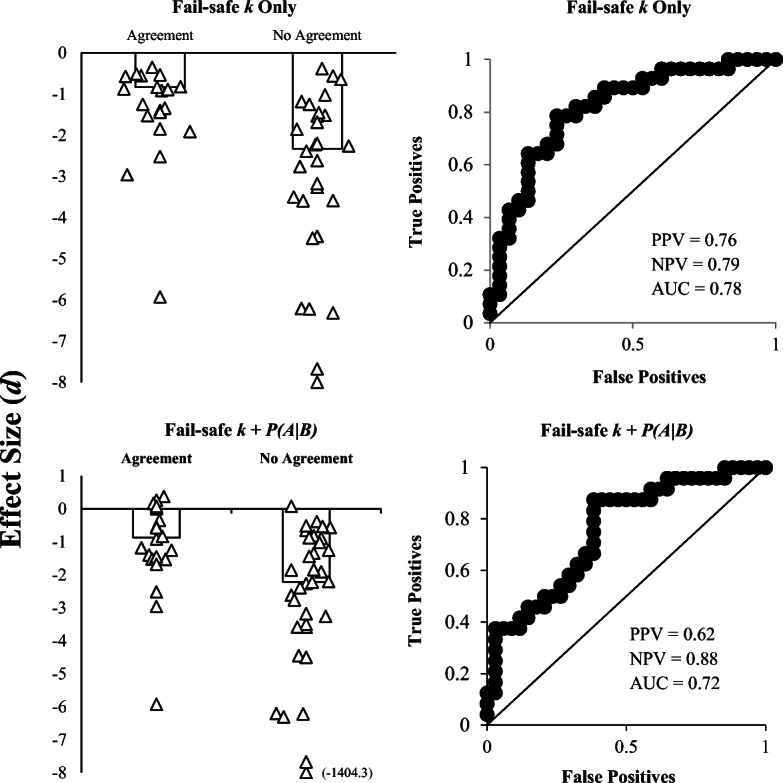
Median d₀ for cases with and without agreement across all three methods (DC, CDC, fail-safe k). Individual data points represent d₀ for individual participants. Agreement with fail-safe k was examined using the fail-safe k rule alone (i.e., k_FS ≤ k_B; top left panel) as well as fail-safe k with subsequent conditional probability analyses (bottom left panel). ROC curves depict d₀ and agreement/disagreement. Each data point represents the sensitivity and 1-specificity values obtained at each d_0. Fail-safe k was examined with (bottom right panel) and without (top right panel) examining the conditional probability of k_FS subsequently occurring if k_FS ≤ k_B

When we evaluated agreement between these methods using FSK in conjunction with conditional probability analyses, the AUC value for d_o (0.72) indicates 72% of cases were correctly identified as either having perfect agreement or disagreement across methods with the empirically derived d of -1.63. These results are consistent with outcomes from the other ROC analyses. Disagreements are more likely to occur when effect sizes are extremely large, and combining FSK with the auxiliary conditional probability analyses actually decreased the predictive value of d_o somewhat. These outcomes indicate that it may not be necessary to calculate the auxiliary conditional probability of subsequent k_FS occurring, as modifying initial decisions based on these analyses may actually decrease agreement between these methods (though the overall level of predictive accuracy is still acceptable and NPV estimates actually increased using this method). This also represents an additional step which clinicians who are using the metric would have to conduct in vivo. It is also possible that using the conditional probability calculations to inform fail-safe k decisions may have enhanced agreement with different cutoff criteria—our 5% cutoff may have been unnecessarily conservative; thus, future researchers should investigate this question.

Taken together, these results broadly suggest that there may be acceptable correspondence between FSK and the DC/CDC methods with small to relatively large effect sizes. However, there is more likely to be disagreement between these three methods when effect sizes are very large. Though this difference seems less likely to affect treatment decisions because visual inspection should lend itself well to evaluating large treatment effects, it does raise questions about why this pattern emerged. One potential explanation may involve the number of data points occurring in Phase B. At the specific probability (p = 0.5) incorporated into the binomial probability calculations, shorter treatment phases (i.e., containing three or four points) will not yield p ≤ .05 even if all points fall below both mean and trend lines due to the binomial probability constraints. This is also consistent with extant literature (Falligant et al., 2019; Lanovaz et al., 2017), which suggests that false positives are relatively probable when Phase B contains only three or four points (regardless of the number of points in Phase A). Thus, it is possible that FSK may be advantageous to use when working with shorter data series. Nonetheless, it is possible that relatively few points in Phase B could be indicative of very large treatment effects (i.e., only three or four points were conducted because the treatment effect was so evident through visual analysis), but still yield outcomes indicating more sessions should be conducted via DC and CDC (but not fail-safe k). To assess this possibility, we conducted follow-up analyses in which we interpreted DC and CDC outcomes (for B Phases containing three of four points) using a more liberal metric—if all points fell below both lines, we concluded additional sessions were not required to demonstrate an effect. It is interesting that this modification only marginally enhanced agreement between the three methods from 50% to 66% when FSK was used in conjunction with the conditional probability analyses. Agreement remained very low when FSK did not include the auxiliary conditional probability analyses (41%).

Future researchers should further examine variables that mediate the generality of the FSK metric, identifying contextual variables (e.g., number of sessions in A and B Phases, type of intervention, functional class of behavior, histories of reinforcement) that make agreement between this and other structured criteria metrics more or less likely. In addition, there may be other criteria that may be used to refine or better quantify the relation between k_fs and k_b (above and beyond evaluating if k_fs > k_b; see Barnard-Brak et al., 2018). Indeed, a ripe area of future research may be to examine how changes to different parameters of this model (e.g., different d_c values, different alpha cutoffs with the Bayesian conditional probability analyses, different criteria for evaluating the relation between K_fs and K_b) affect the utility of this model in different clinical contexts and data sources. For example, additional research should also examine how FSK estimates differ when using sample-specific d_c values (i.e., derived from the clinical dataset of interest, and/or using d_c values which correspond to a minimum 80% reduction in problem behavior) in lieu of the d_c provided by Barnard-Brak et al. Given that there are many ways to calculate effect size for SCEDs (regression-based and nonregression-based; e.g., Parker et al., 2011), it may be possible to further enhance the utility of this metric using different methods for estimating effect size. This will be an important step, because one reason for using structured criteria/statistical analyses within SCEDs is to communicate findings with clinicians and researchers from other fields. For this reason, it may also be important to formally examine if/how use of structured criteria (including DC/CDC and FSK) increase transparency and communication with other fields that are less likely to rely on visual analysis or use different estimates of effect size. In the meantime, these results provide limited support for use of this tool with nonpublished clinical data, in particular when evaluating small or medium-to-large treatment effects. However, the excellent correspondence between DC and CDC suggest these procedures should continue to be favored while FSK methodological questions continue to be examined and clarified. That said, there are also a number of potential limitations to using DC and CDC that must be considered, including the limiting impact of data series length and autocorrelation (Manolav & Solanas, 2008) that might make fail-safe k more desirable for some.

Of course, there may be exceptions to these recommendations for some clinicians and researchers. Regardless of which structured criteria are used to complement visual inspection, clinicians should rely on clinical judgement when making decisions regarding conducting additional treatment sessions or changing phases—in other words, quantitative structured criteria should be used to enhance or support clinical decision making, but not supplant it. This pertains to well-established structured criteria (i.e., dual-criteria methods) but is especially true for relatively untested tools such as FSK. Behavioral treatments are provided on an individualized basis, meaning that estimates of “clinically significant” effects derived from aggregated clinical datasets (i.e., d_c) may not correspond to effects that are meaningful on an individual level. Nonetheless, there are accepted benchmarks for behavior reduction that are commonly used in applied behavior analysis. For example, an 80% reduction in problem behavior relative to baseline is benchmark for positive response to treatment (e.g., Greer, Fisher, Saini, Owen, & Jones, 2016; Hagopian, Fisher, Sullivan, Acquisto, & LeBlanc, 1998). Of course, such measures of efficacy are only meant to capture relatively large changes in behavior and do not necessarily reflect broader behavioral changes or treatment targets. As a corollary, FSK values and the estimates of effect size from which they are derived may not perfectly reflect data series stability and clinically significant decreases in target behavior, but they may help clinicians determine how to proceed under clinical ambiguity (if future research in this area provides additional support for this approach).

Findings of the current investigation add to the limited extant FSK literature in several ways by demonstrating (1) agreement between FSK and DC/CDC was not uniformly high (or even particularly good); however, agreement was more likely to occur when effect sizes were small to moderate, which is an encouraging finding for FSK proponents; (2) the auxiliary conditional probability analyses outlined by Barnard-Brak et al. (2018) may not be necessary to conduct when calculating and interpreting FSK values; and (3) DC/CDC may be more conservative (i.e., indicate additional sessions should be conducted) relative to FSK when Phase B only contains three or four data points (consistent with Lanovaz et al., 2017). Given the aforementioned questions regarding the utility, feasibility, and methodological concerns associated with FSK, future research must examine and clarify these issues before these procedures are used within the field by practitioners. Thus, although our results provide some degree of support for use of this approach as a research tool with clinical data, in particular when evaluating small or medium treatment effect sizes, further research is needed before this is used clinically. It is hoped that the results from the current study provide multiple avenues for additional research regarding the utility and practicality of FSK (as well as DC and CDC). Within the current study, we have demonstrated that agreement between FSK and DC/CDC is generally poor, and provided a number of potential reasons why this may be the case. The next step will be to identify why this is the case, and examine specific conditions under which agreement is (or is not) enhanced. It is plausible that each method has distinct advantages and disadvantages that confer clinical utility depending on a number of clinical-contextual factors. At present, the research on FSK specifically (and other quantitative structured criteria broadly) is nascent and precludes definitive conclusions about the place of these tools within the scope of clinical application. These outcomes highlight emerging issues and area of disagreement in the field regarding the role of quantitative structured criteria in applied behavior analysis.

References

- Baer DM. Perhaps it would be better not to know everything. Journal of Applied Behavior Analysis. 1977;10:167–172. doi: 10.1901/jaba.1977.10-167. [DOI] [PMC free article] [PubMed] [Google Scholar]
- Barnard-Brak L, Richman DM, Little TD, Yang Z. Development of an in-vivo metric to aid visual inspection of single-case design data: Do we need to run more sessions? Behaviour Research and Therapy. 2018;102:8–15. doi: 10.1016/j.brat.2017.12.003. [DOI] [PubMed] [Google Scholar]
- Brossart DF, Parker RI, Olson EA, Mahadevan L. The relationship between visual analysis and five statistical analyses in a simple AB single-case research design. Behavior Modification. 2006;30:531–563. doi: 10.1177/0145445503261167. [DOI] [PubMed] [Google Scholar]
- Carr JE, Coriaty S, Wilder DA, Gaunt BT, Dozier CL, Britton LN, et al. A review of “noncontingent” reinforcement as treatment for the aberrant behavior of individuals with developmental disabilities. Research in Developmental Disabilities. 2000;21:377–391. doi: 10.1016/S0891-4222(00)00050-0. [DOI] [PubMed] [Google Scholar]
- Carr JE, Severtson JM, Lepper TL. Noncontingent reinforcement is an empirically supported treatment for problem behavior exhibited by individuals with developmental disabilities. Research in Developmental Disabilities. 2009;30:44–57. doi: 10.1016/j.ridd.2008.03.002. [DOI] [PubMed] [Google Scholar]
- Falligant, J. M., McNulty, M. K., Hausman, N. L., & Rooker, G. W. (2019). Using dual-criteria methods to supplement visual inspection: Replication and extension. Journal of Applied Behavior Analysis. [DOI] [PubMed]
- Fisher WW, Kelley ME, Lomas JE. Visual aids and structured criteria for improving visual inspection and interpretation of single-case designs. Journal of Applied Behavior Analysis. 2003;36:387–406. doi: 10.1901/jaba.2003.36-387. [DOI] [PMC free article] [PubMed] [Google Scholar]
- Fisher, W. W., & Lerman, D. C. (2014). It has been said that, “There are three degrees of falsehoods: Lies, damn lies, and statistics.” Journal of School Psychology, 52, 243–248. 10.1016/j.jsp.2014.01.001 [DOI] [PubMed]
- Gage NA, Lewis TJ. Hierarchical linear modeling meta-analysis of single-subject design research. Journal of Special Education. 2014;48:3–16. doi: 10.1177/0022466912443894. [DOI] [Google Scholar]
- Greer BD, Fisher WW, Saini V, Owen TM, Jones JK. Functional communication training during reinforcement schedule thinning: An analysis of 25 applications. Journal of Applied Behavior Analysis. 2016;49:105–121. doi: 10.1002/jaba.265. [DOI] [PMC free article] [PubMed] [Google Scholar]
- Hagopian LP, Fisher WW, Sullivan MT, Acquisto J, LeBlanc LA. Effectiveness of functional communication training with and without extinction and punishment: A summary of 21 inpatient cases. Journal of Applied Behavior Analysis. 1998;31:211–235. doi: 10.1901/jaba.1998.31-211. [DOI] [PMC free article] [PubMed] [Google Scholar]
- Hagopian LP, Fisher WW, Thompson RH, Owen-DeSchryver J, Iwata BA, Wacker DP. Toward the development of structured criteria for interpretation of functional analysis data. Journal of Applied Behavior Analysis. 1997;30:313–326. doi: 10.1901/jaba.1997.30-313. [DOI] [PMC free article] [PubMed] [Google Scholar]
- Hagopian LP, Rooker GW, Yenokyan G. Identifying predictive behavioral markers: A demonstration using automatically reinforced self-injurious behavior. Journal of Applied Behavior Analysis. 2018;51:443–465. doi: 10.1002/jaba.477. [DOI] [PMC free article] [PubMed] [Google Scholar]
- Harrington M, Velicer WF. Comparing visual and statistical analysis in single-case studies using published studies. Multivariate Behavioral Research. 2015;50:162–183. doi: 10.1080/00273171.2014.973989. [DOI] [PMC free article] [PubMed] [Google Scholar]
- Kyonka EG, Mitchell SH, Bizo LA. Beyond inference by eye: Statistical and graphing practices in JEAB, 1992-2017. Journal of the Experimental Analysis of Behavior. 2019;111:155–165. doi: 10.1002/jeab.509. [DOI] [PubMed] [Google Scholar]
- Lanovaz MJ, Huxley SC, Dufour MM. Using the dual-criteria methods to supplement visual inspection: An analysis of nonsimulated data. Journal of Applied Behavior Analysis. 2017;50:662–667. doi: 10.1002/jaba.394. [DOI] [PubMed] [Google Scholar]
- Lenz AS. Calculating effect size in single-case research: A comparison of nonoverlap methods. Measurement & Evaluation in Counseling & Development. 2013;46:64–73. doi: 10.1177/0748175612456401. [DOI] [Google Scholar]
- Manolov R, Solanas A. Comparing N = 1 effect size indices in presence of autocorrelation. Behavior Modification. 2008;32:860–875. doi: 10.1177/0145445508318866. [DOI] [PubMed] [Google Scholar]
- Ninci J, Vannest KJ, Willson V, Zhang N. Interrater agreement between visual analysts of single-case data: A meta-analysis. Behavior Modification. 2015;39:510–541. doi: 10.1177/0145445515581327. [DOI] [PubMed] [Google Scholar]
- Parker RI, Vannest KJ, Davis JL. Effect size in single-case research: A review of nine nonoverlap techniques. Behavior Modification. 2011;35:303–322. doi: 10.1177/0145445511399147. [DOI] [PubMed] [Google Scholar]
- Phillips CL, Iannaccone JA, Rooker GW, Hagopian LP. Noncontingent reinforcement for the treatment of severe problem behavior: An analysis of 27 consecutive applications. Journal of Applied Behavior Analysis. 2017;50:357–376. doi: 10.1002/jaba.376. [DOI] [PMC free article] [PubMed] [Google Scholar]
- Roane HS, Fisher WW, Kelley ME, Mevers JL, Bouxsein KJ. Using modified visual-inspection criteria to interpret functional analysis outcomes. Journal of Applied Behavior Analysis. 2013;46:130–146. doi: 10.1002/jaba.13. [DOI] [PubMed] [Google Scholar]
- Sham E, Smith T. Publication bias in studies of an applied behavior-analytic intervention: An initial analysis. Journal of Applied Behavior Analysis. 2014;47:663–678. doi: 10.1002/jaba.146. [DOI] [PubMed] [Google Scholar]
- Stewart KK, Carr JE, Brandt CW, McHenry MM. An evaluation of the conservative dual-criterion method for teaching university students to visually inspect AB-design graphs. Journal of Applied Behavior Analysis. 2007;40:713–718. doi: 10.1901/jaba.2007.713-718. [DOI] [PMC free article] [PubMed] [Google Scholar]
- Smith JD. Single-case experimental designs: A systematic review of published research and current standards. Psychological Methods. 2012;17:510–550. doi: 10.1037/a0029312. [DOI] [PMC free article] [PubMed] [Google Scholar]
- Tarlow KR, Brossart DF. A comprehensive method of single-case data analysis: Interrupted Time-Series Simulation (ITSSIM) School Psychology Quarterly. 2018;33:590–560. doi: 10.1037/spq0000273. [DOI] [PubMed] [Google Scholar]
- Thompson RH, Iwata BA, Hanley GP, Dozier CL, Samaha AL. The effects of extinction, noncontingent reinforcement, and differential reinforcement of other behavior as control procedures. Journal of Applied Behavior Analysis. 2003;36(2):221–238. doi: 10.1901/jaba.2003.36-221. [DOI] [PMC free article] [PubMed] [Google Scholar]
- Wolery M, Busick M, Reichow B, Barton EE. Comparison of overlap methods for quantitatively synthesizing single-subject data. Journal of Special Education. 2010;44:18–28. doi: 10.1177/0022466908328009. [DOI] [Google Scholar]
- Wolfe K, Seaman MA, Drasgow E, Sherlock P. An evaluation of the agreement between the conservative dual-criterion method and expert visual analysis. Journal of Applied Behavior Analysis. 2018;51:345–351. doi: 10.1002/jaba.453. [DOI] [PubMed] [Google Scholar]