

Abstract
Multi‐channel phased receive arrays have been widely adopted for magnetic resonance imaging (MRI) and spectroscopy (MRS). An important step in the use of receive arrays for MRS is the combination of spectra collected from individual coil channels. The goal of this work was to implement an improved strategy termed OpTIMUS (i.e., optimized truncation to integrate multi‐channel MRS data using rank‐R singular value decomposition) for combining data from individual channels. OpTIMUS relies on spectral windowing coupled with a rank‐R decomposition to calculate the optimal coil channel weights. MRS data acquired from a brain spectroscopy phantom and 11 healthy volunteers were first processed using a whitening transformation to remove correlated noise. Whitened spectra were then iteratively windowed or truncated, followed by a rank‐R singular value decomposition (SVD) to empirically determine the coil channel weights. Spectra combined using the vendor‐supplied method, signal/noise2 weighting, previously reported whitened SVD (rank‐1), and OpTIMUS were evaluated using the signal‐to‐noise ratio (SNR). Significant increases in SNR ranging from 6% to 33% (P ≤ 0.05) were observed for brain MRS data combined with OpTIMUS compared with the three other combination algorithms. The assumption that a rank‐1 SVD maximizes SNR was tested empirically, and a higher rank‐R decomposition, combined with spectral windowing prior to SVD, resulted in increased SNR.
Keywords: magnetic resonance spectroscopy, phased array combination, signal‐to‐noise, singular value decomposition
Optimized truncation to integrate multi‐channel MRS data using rank‐R singular value decomposition (OpTIMUS) is an improved strategy for combining MRS data collected from multi‐channel phased receive arrays that uses a rank‐R decomposition and spectral windowing prior to singular value decomposition (SVD). Spectra combined using OpTIMUS, whitened singular value decomposition (WSVD), signal/noise2 (S/N2) weighting, and the vendor‐supplied method were evaluated using SNR. In vivo spectra combined with OpTIMUS had significantly higher SNR compared with the other three methods.
Abbreviations used
- CHESS
chemical shift selective saturation
- Cho
choline
- Cr
creatine
- FDR
false discovery rate
- Glu
glutamate
- Lac
lactate
- LFWM
left frontal white matter
- mI
myo‐inositol
- MPRAGE
magnetization‐prepared rapid gradient‐echo
- MSE
mean squared error
- NAA
N‐acetylaspartate
- OpTIMUS
optimized truncation to integrate multi‐channel MRS data using rank‐R singular value decomposition
- PCA
principal component analysis
- PCC
posterior cingulate cortex
- PRESS
point‐resolved spectroscopy
- PSD
power spectral density
- RFWM
right frontal white matter
- S/N2
signal/noise2
- SD
standard deviation
- SNR
signal‐to‐noise ratio
- SVD
singular value decomposition
- SVS
single voxel spectroscopy
- Tx‐OFF
transmission pulse off
- Tx‐ON
transmission pulse on
- WSVD
whitened singular value decomposition
1. INTRODUCTION
Magnetic resonance spectroscopy (MRS) is an important noninvasive tool for quantifying local chemical and metabolic changes. However, clinical applications of MRS are often limited by the low signal‐to‐noise ratio (SNR). 1 , 2 , 3 The use of multi‐channel phased receive arrays for parallel imaging in MRS is a current strategy for addressing these challenges and accelerating acquisition times. 4 , 5 , 6 , 7 A key step in the use of multi‐channel receive arrays for MRS is properly combining individual MR spectra from each coil channel. Previously reported combination algorithms have resulted in inconsistent improvements in spectral resolution and SNR, as combining the data from phased array coils can introduce artifacts due to noise or peak distortions. 1 , 2 , 3 , 7 , 8 Spectral noise can be classified as either extrinsic or intrinsic noise. Extrinsic noise arises from correlated signal or voltage due to mutual impedance between coil elements. 9 , 10 Intrinsic noise results from thermal fluctuations in the coil elements (Johnson noise), eddy currents in the thermally conducting sample, and other sources of physiological noise. 4 , 9 , 10 , 11
Several spectral combination methods have been proposed to maximize SNR, utilizing both calculated coil sensitivity or field maps and data‐driven approaches. 7 , 12 , 13 , 14 , 15 The seminal paper by Roemer et al proposed a sum‐of‐squares combination method to remove mutual inductance (signal transfer between coupled coil channels) and mutual resistance (due to coupled hardware and resistance from the conducting sample) by quantifying the correlation of noise between the coils. 4 The sum‐of‐squares method ignores noise correlation and does not use prior knowledge to generate a coil sensitivity map as the exact position of the coils and phase of the signal are not always known.
An alternative method derived from the sum‐of‐squares approach was the use of singular value decomposition (SVD) for spectral combination. 16 Erdogmus et al demonstrated that the combination of pixel values from MRI data and prior information to derive coil sensitivities resulted in higher SNR due, in part, to the removal of noise when using a rank‐1 approximation for the measurement matrix. While the SVD method was promising initially, Bydder et al identified limitations of the implementation of SVD for coil combination. 17 In particular, many SVD formulations assume noise between coils is uncorrelated with equal variance; however, in practice this assumption is violated.
Rodgers and Robson proposed a refined SVD‐based combination referred to as whitened SVD (WSVD). 13 , 18 WSVD uses the following steps for multi‐channel signal combination: (1) decorrelating the extrinsic noise from a noise covariance matrix of the array coils and (2) applying the SVD algorithm to find suitable coil weights for combination. Improved SNR was reported for WSVD compared with the method proposed by Brown that utilizes both noise and spectral amplitude to optimize coil weights. 19 Importantly, most implementations of SVD, including WSVD, treat the final combined matrix as the first left singular vector or a rank‐1 decomposition. Theoretically, if noise whitening produces completely isotropic noise, the variance of the metabolite signal will be best represented by the direction of maximum variance (i.e., a rank‐1 SVD). However, this is in general not equivalent to maximizing the SNR of the metabolites. Moreover, in cases where noise whitening is imperfect, a portion of the signal may be present in higher order vectors. Then a rank‐R SVD combined with spectral windowing may better represent the key spectral features and improve SNR.
This motivates a novel method that seeks to maximize the SNR of the metabolites rather than the variance contained in the first component. Here, we present a new SVD‐based combination method that utilizes optimized truncation to integrate multi‐channel MRS data using rank‐R singular value decomposition (OpTIMUS). The metabolite subspace used to maximize SNR of the combined spectrum is determined by truncating or windowing the individual spectra followed by iterative rank‐R SVD. 20 Significant increases in SNR without compromising metabolite quantification were observed in the combined spectra using OpTIMUS compared with several previously reported methods, including the method used by the scanner manufacturer.
2. THEORY
2.1. Spectral noise
Let Z denote the true signal, and S denote the measured M × N matrix where M is the number of complex data points (e.g., 1024) and N is the number of coil elements in the phased array (e.g., 32). Let E denote the M × N complex‐valued extrinsic noise. Let α denote a complex vector of dimension N, where αHα = 1 denotes the coil sensitivities using the singular vector definition, and H is the Hermitian transpose. The measured data can then be described as
| (1) |
Let represent the complex noise covariance matrix and , where is a unitary matrix with eigenvectors of noise covariance and is a diagonal matrix of eigenvalues. The covariance matrix can be calculated from either a noise‐only scan or noise‐only region of the spectrum, with the caveat that enough noise samples must be acquired to precisely estimate the noise covariance matrix (Methods). 18 Using principal component analysis (PCA) to whiten the noise, 21 the eigenvalue decomposition can be used to rotate the original spectral data for noise decorrelation with , followed by scaling to whiten the data using the diagonal matrix, Starting with the unwhitened spectra containing correlated noise, S (M × N matrix), the noise whitening matrix ) can produce whitened spectra, . Using the same notation as Equation 1,
| (2) |
Note that this results in isotropic noise:
| (3) |
Define and let . Denote the whitened noise as and define (complex vector of dimension N). The covariance of the whitened spectra can then be derived as
| (4) |
In this formulation, the covariance is composed of the sum of three rank‐1 terms plus the isotropic error variance. (Here we use the term “covariance” to simplify the discussion, although in a statistical treatment, is the covariance plus the outer product of the means.) If γβH = 0, then in the eigenvalue decomposition of , the first eigenvector would be β, as this is the only direction in the complex space across N that contains additional variance. In practice, this is approximately true when , e.g., the signal and noise are uncorrelated.
2.2. Coil combination using SVD
Previous work using the SVD formulation assumed the rank‐1 decomposition. The SVD of the whitened spectral matrix, , is
| (5) |
where U is an M × M matrix of left singular vectors, Σ is a diagonal matrix containing the singular values of , and V is an N × N matrix of right singular vectors. Let V = [V1, V2, …, VN]. Assuming , β is the direction containing the largest variance according to Equation 4. Hence
| (6) |
where ‖β‖ denotes the Euclidean norm. Using the same formulation in Equation 1, the SVD for the rank‐1 projection is
| (7) |
| (8) |
| (9) |
where Equation 9 represents the scaled true signal, Z‖β‖, plus the noise that is not orthogonal to the rotated coil sensitivities, . This noise is nonzero as the whitened noise has unit variance in all directions including V1, and , so there will be nontrivial corruption of the true signal. Thus, if were known, and the same coil sensitivities apply to all frequencies as in Equation 1, the rank‐1 SVD contains the signal.
The first observation is that the equivalence between the first singular vector V1 and the rotated and scaled sensitivities β/‖β‖ in Equation 6 does not hold when the estimate of the noise covariance matrix is not equal to . In practice, the noise E is not directly observed. Instead, it is estimated from noise data using a noise‐only scan or noise‐only region of the spectrum, leading to an estimate . These approaches implicitly assume the noise data points are realizations from a population covariance matrix C. Taking more noise samples would lead to converging to C; however, it does not guarantee that is more similar to . Note that is unknowable in practice, since it is the realization of noise that occurs when the data are collected. As shown in Equation 4, it is , not or C, that perfectly allocates the signal to the first singular vector, such that the prewhitening in general cannot be perfect. In addition to sampling variation leading to differences between and , there may be more systematic differences due to different noise characteristics of . For example, noise characteristics from a noise‐only scan may differ from those calculated using a noise‐only region of the spectrum when the transmitter is on. Imperfect whitening results in anisotropy, which can result in a noise direction of variance impacting the first singular vector of the SVD. Then the rank‐1 projection in Equation 7 can result in signal in higher rank components and an unequal distribution of the noise across singular vectors. Another factor that can impact the decomposition is the assumption .
The second observation is that the rank‐1 representation from the SVD is equivalent to finding the direction that maximizes the variance. Maximizing the variance in general is not equivalent to maximizing the SNR, where SNR is defined as the reference metabolite peak divided by the standard deviation (SD) of the noise region. We propose to use SNR as the objective function, which we maximize using a combination of a rank‐R decomposition and a windowed approach to the SVD. This may improve the representation of metabolites by finding the coil combination that best represents metabolite peaks relative to the noise. The final observation is that across the spatial extent of the voxel, there may exist differences in coil sensitivities, which would lead to violations of Equation 1.
2.3. OpTIMUS implementation
In OpTIMUS, whitened spectral data points are iteratively windowed to find the optimal spectral window (L data points) and generate a new L × N matrix, , and the economy (or thin) SVD is then performed on the windowed or truncated matrix,
| (10) |
All spectral windows with a minimum matrix size or rank equal to the number of coils (i.e., 32) were considered when determining the maximum SNR from a rank‐R decomposition of the whitened windowed matrix (L × N). As L is equal to or greater than N, the economy SVD was used to reduce computational load by only calculating the first N singular values of L. 22 After SVD is performed on a spectral window, R was determined by systematically evaluating the rank decomposition (rank‐1 to rank‐N) that produces the maximum SNR value. SNR was calculated using the N‐acetylaspartate (NAA) peak as well as a weighted average of NAA (2.0 ppm), choline (Cho, 3.2 ppm), and creatine (Cr, 3.0 ppm) peaks. The coil combination matrix, , and the diagonal singular value matrix, , which produces the weights for each rank (rank‐1 to rank‐R), are then applied to the full spectrum to calculate the linearly combined rank‐1 spectrum, , using
| (11) |
3. METHODS
3.1. MR experiments
All MR experiments were performed on a whole‐body 3 T MR scanner (MAGNETOM PrismaFit, Siemens Healthcare, Erlangen, Germany) using a 32‐channel phased array head coil. A T1 weighted magnetization‐prepared rapid gradient‐echo (MPRAGE) sequence (TR/TI/TE = 2300/900/3.39 ms, flip angle = 9°, field of view = 256 mm × 256 mm, matrix size = 192 × 192, 160 slices, slice thickness = 1 mm) was used to obtain anatomical images for positioning the MRS voxel (2 × 2 × 2 cm3 nominal voxel size). Single voxel 1H spectroscopy (SVS) data were collected using the point‐resolved spectroscopy (PRESS) sequence (TR/TE = 1700/35 ms, 1024 complex data points, 1200 Hz bandwidth, 128 signal averages, and chemical shift selective saturation (CHESS)‐based water suppression with 50 Hz bandwidth). A noise‐only scan was collected by setting the amplitude of all RF transmission pulses to zero (Tx‐OFF) and the receiver gain set to high during acquisition. With the exception of the transmission pulses, all other parameters were identical. The Tx‐OFF scan was used to remove extrinsic noise via the whitening transformation.
3.1.1. Data collection in healthy human subjects
This study was approved by the Institutional Review Board of Emory University. Eleven healthy human subjects (10 males and one female; mean ± SD age = 24 ± 5 years old) were included in the study and subjects provided written informed consent prior to MR scans. Subjects were positioned head‐first and supine in the scanner with their head immobilized in the phased array coil with foam padding to minimize motion. 1H MRS was performed in the brain at three voxel positions: left frontal white matter (LFWM), right frontal white matter (RFWM), and posterior cingulate cortex (PCC) (Figure 1).
FIGURE 1.
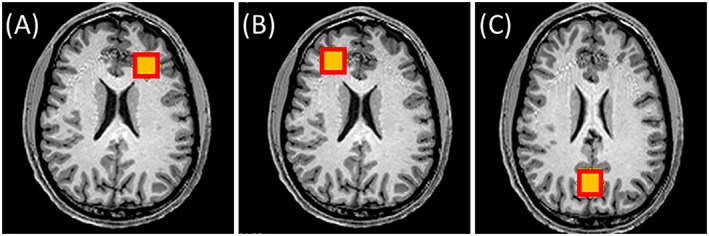
Voxel positions for 1H MRS acquired in healthy human subjects overlaid on T1‐weighted axial MPRAGE images. Images are presented in the radiological convention and spectra were collected in the (A) left frontal white matter, (B) right frontal white matter, and (C) posterior cingulate cortex
3.1.2. Data collection in a brain spectroscopy phantom
To determine the effect of the coil combination method on accurate metabolite quantification, 1H MRS data were collected from a spherical brain spectroscopy phantom (Braino phantom, #2152220, GE Healthcare, Chicago, IL) containing 12.5 mM of NAA, 10 mM of Cr, 3 mM of Cho, 7.5 mM of myo‐inositol (mI), 12.5 mM of L‐glutamic acid (Glu), 5 mM of DL‐lactic acid (Lac), sodium azide (0.1%), 50 mM of potassium phosphate monobasic, 56 mM of sodium hydroxide (NaOH), and 1 mL/L of Gd‐DPTA (Magnevist). 23 MRS data were acquired during three separate scan sessions using 5‐6 different voxel positions/session for a total of 16 unique spectra of metabolites with known concentrations that were used to determine the accuracy of metabolite quantification after combination. A multi‐compartment phantom was also constructed to test for out‐of‐volume artifacts. The phantom was composed of two nested cylinders with an inner compartment containing 5 mM NAA and an outer compartment containing only water.
3.2. Coil combination using OpTIMUS
3.2.1. Noise whitening
Noise decorrelation, or whitening, was performed on the full uncombined spectral matrix (Equation 2). In vivo data were whitened using the Tx‐OFF scan collected with 1024 complex data points and 128 averages. A total of >130 000 noise points were collected from each coil to enable precise estimation of the noise covariance matrix, based on previous simulations showing that 105 noise samples are required for convergence. 18 The whitening matrix was calculated from the complex noise covariance matrix, (Section 2.1).
3.2.2. Spectral windowing and rank‐R decomposition
A schematic illustration of the OpTIMUS method is presented in Figure 2. OpTIMUS uses a linear combination of a rank‐R decomposition, in which optimal rank size was determined for each spectral window. SNR of the final combined spectrum was used as the objective function. After the SVD is performed on the windowed spectra, as described in Section 2.3, the stored rank size is then used to sum the singular vectors from each rank using the singular value weights (Equation 11). Pseudocode detailing the iterative process to determine the rank and window size are included in the supporting information (Figure S1).
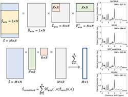
FIGURE 2.
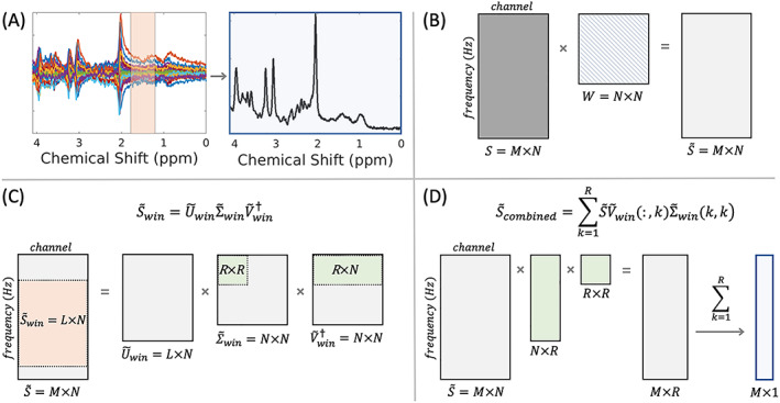
Schematic illustration of OpTIMUS. (A) Representative spectra from 32 coil channels (left) combined into a single spectrum (right) using an optimized spectral window (orange shaded region) and rank‐R SVD to determine the coil weights. The primary steps in OpTIMUS include: (B) whitening the spectral matrix, S, containing M spectral data points and N coil channels, using W (see text, Section 2.1) to produce a whitened spectral matrix, ; (C) spectral windowing of the noise‐whitened matrix to produce an L x N matrix, (orange), followed by iterative rank‐R economy SVD on the windowed matrix (green boxes); and (D) combination of the M x R low‐rank matrix using the coil combination right singular vectors determined from the rank‐R SVD of (green boxes) to generate an SNR‐optimized, rank‐1 combined spectrum, (blue)
3.3. Spectral and statistical analysis
Data analysis was performed in MATLAB (R2019a, MathWorks, Natick, MA). Values are reported as the mean ± SD, unless specified otherwise. Unprocessed raw measurement (Siemens twix) data from each coil were converted to a MATLAB structure array using the GannetLoad function in Gannet 3.0, 24 and the raw data were combined using OpTIMUS, WSVD, and S/N2 weighting. The performance of the combination methods was evaluated using the SNR of the final combined spectrum. Spectra were normalized by dividing the entire spectrum by the real value of the NAA peak. Normalization accounted for differences in the dynamic spectral range as a result of the combination method. SNR of the OpTIMUS combined spectra were compared with the vendor‐supplied method, S/N2 weighting, 25 and WSVD. 18 SNR was calculated from the NAA peak amplitude divided by the SD of the noise‐only region between 8.43‐9.34 ppm. SNR was also calculated using an amplitude‐weighted average of the SNR calculated from the NAA, Cho, and Cr peaks to determine if the results were dependent on the peak chosen for SNR optimization.
To determine the effect of the coil combination method on metabolite quantification, NAA, Cho, and Cr peaks in the combined phantom spectra were integrated following peak fitting using a Voigt lineshape. 26 The accuracy of metabolite concentration ratios, normalized to Cr, are reported as the squared difference between estimated and known concentrations (Section 3.1.2), such that the average of these differences is the mean squared error (MSE). Differences in accuracy between methods were evaluated using the Wilcoxon test.
Statistical comparisons of the combination methods were performed using linear mixed models, in which SNR was the response variable, and voxel position (LFWM, RFWM, PCC), method (OpTIMUS, WSVD, S/N2 weighting, and vendor‐supplied), and their interaction were included as main effects. The inclusion of random effects due to subject, voxel nested in subject, and method nested in subject were evaluated. The random effects account for correlations due to repeated measurements on subjects, voxels, and/or methods. Normality of residuals was assessed visually. Using Akaike information criterion corrected for small sample size, we selected a model with random intercepts for subject and the interaction between voxel and subject. P‐values were calculated using the Kenward‐Roger approach to estimate degrees of freedom. P‐values were corrected for multiple comparisons (comparing three methods with OpTIMUS for each of three voxels, or nine tests) using the false discovery rate (FDR). 27 P‐values ≤0.05 were considered significant. All statistical analyses were performed in R using the packages lme4, 28 AICcmodavg, 29 and emmeans. 30
4. RESULTS
4.1. Improved SNR of brain MRS data using OpTIMUS
Significant improvements in SNR were observed for OpTIMUS compared with WSVD, S/N2 weighting, and the vendor‐supplied method (Table 1). For each voxel position, OpTIMUS generated significantly higher SNR values compared with all three other methods. Representative brain spectra acquired in the LFWM and following combination with each algorithm are shown in Figure 3. OpTIMUS‐combined spectra (Figure 3A) had the highest SNR compared with the other three combination algorithms (Figures 3B‐D). While SNR was calculated using the NAA peak, similar improvements were observed for SNR calculated using an amplitude‐weighted average of the NAA, Cho, and Cr peaks (Table S1).
TABLE 1.
SNR of combined spectra using four different combination algorithms, as a function of voxel position, averaged across all subjects (mean ± SD)
| LFWM | RFWM | PCC | |||||||
|---|---|---|---|---|---|---|---|---|---|
| SNR | SNR change a [%] | P‐value b | SNR | SNR change [%] | P‐value | SNR | SNR change [%] | P‐value | |
| OpTIMUS | 141.88 ± 39.63 | ― | ― | 146.31 ± 35.19 | ― | ― | 180.73 ± 49.48 | ― | ― |
| WSVD | 128.11 ± 35.93 | −9.70 | 0.038* | 128.06 ± 31.38 | −12.47 | 0.004* | 159.09 ± 41.54 | −11.97 | <0.001* |
| S/N2 | 94.31 ± 17.46 | −33.53 | <0.001* | 111.32 ± 31.92 | −23.91 | <0.001* | 131.04 ± 36.05 | −27.50 | <0.001* |
| Vendor | 112.25 ± 32.60 | −20.88 | <0.001* | 126.20 ± 34.18 | −13.74 | 0.002* | 169.05 ± 34.59 | −6.47 | 0.038* |
Abbreviations: LFWM, left frontal white matter; PCC, posterior cingulate cortex; RFWM, right frontal white matter; S/N2, signal/noise2 weighting; Vendor, vendor‐supplied method; WSVD, whitened SVD.
SNR change is the % SNR decrease from OpTIMUS.
P‐values are relative to OpTIMUS and corrected for multiple comparisons using the false discovery rate.
P ≤ 0.05 is statistically significant.
FIGURE 3.
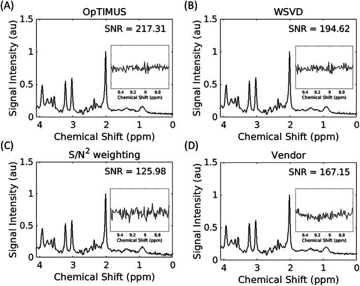
Representative in vivo brain spectra acquired in a left frontal white matter voxel and combined with four different algorithms: (A) OpTIMUS, (B) WSVD, (C) S/N2 weighting, and (D) the vendor‐supplied method. Inset is the noise region between 8.6‐9.6 ppm
4.2. Effect of spectral truncation and rank‐R decomposition
The OpTIMUS algorithm utilizes spectral windowing prior to rank‐R SVD. To identify the effect of these steps on the final spectra, the first three singular vectors for in vivo data, prior to combination, are shown in Figure 4. Using WSVD without windowing, the second and third singular vectors contain higher intensity metabolite peaks in the spectrum, supporting the use of the windowed approach to capture more signal in the first singular vector (which is weighted the highest in the final combined spectrum), as well as a rank‐R rather than rank‐1 decomposition to maximize SNR. We did not observe evidence of out‐of‐volume artifacts due to imperfect PRESS localization (Figure S2). This suggests that our improvements are not simply the result of applying different coil sensitivities to artifacts that have spatially varied receive fields.
FIGURE 4.
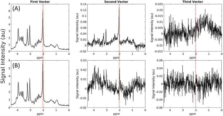
The first three left singular vectors after SVD‐based combination. Spectral rows correspond to: (A) in vivo spectra combined with SVD, without windowing, and (B) in vivo spectra combined with OpTIMUS. Each vector is weighted by the respective singular value. Red vertical lines correspond to the NAA peak (~2.0 ppm)
Previous implementations of the SVD use only the first left singular vector for the combined spectrum as, theoretically, a rank‐1 decomposition will produce the optimal spectrum if noise is decorrelated and isotropic. We observed that for combination of spectra acquired in vivo from human brain tissue, a rank‐1 decomposition was suboptimal. Iterative rank‐determination for each dataset revealed that a decomposition with rank >1 was always required to maximize SNR, with mean rank = 21 across all voxels and subjects. To examine this further, noise power spectral density (PSD) was calculated for each coil channel following noise whitening (Figure 5). While perfect whitening should result in unstructured noise, it is evident that whitening was imperfect for some coils (e.g., coils 17 and 27). As highlighted in Equation 9, nonzero noise or imperfect whitening is expected and leads to signal in higher order singular vectors, providing further support that a rank‐R decomposition may increase spectral SNR.
FIGURE 5.
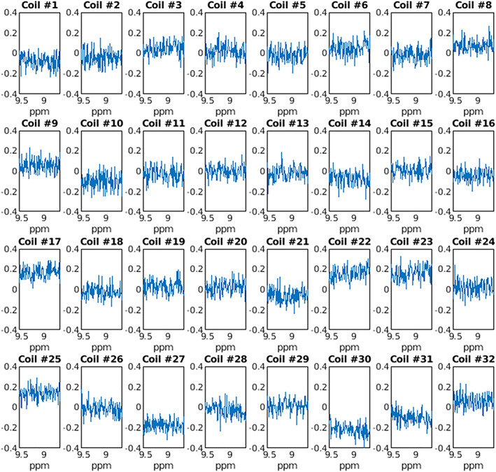
Noise PSD for each coil channel after whitening. While noise has a mean approximately equal to zero for many coil channels, several channels have nonzero means suggesting evidence of imperfect whitening (e.g., coil 17, 27, 30)
4.3. Metabolite quantification
To confirm that increased SNR after combination with OpTIMUS does not compromise metabolite quantification, calculated metabolite ratios of NAA/Cr, Cho/Cr, and mI/Cr from repeated measurements in a brain phantom were compared with the known metabolite ratios. MSE calculated from spectra combined with OpTIMUS and the vendor‐supplied method, respectively, were 0.0134 and 0.023 (NAA/Cr), 0.00020 and 0.00022 (Cho/Cr), and 0.0062 and 0.0063 (mI/Cr). The MSE for NAA/Cr was significantly reduced using OpTIMUS compared with the vendor‐supplied method (P = 0.02). MSE for other methods did not vary significantly (P > 0.05).
5. DISCUSSION
OpTIMUS is an SVD‐based combination algorithm for MR spectra acquired from multi‐channel phased array coils that relies on empirical determination of both the spectral window used to calculate coil weights and the optimal rank‐R decomposition. Compared with WSVD, 18 S/N2 weighting, 25 and the vendor‐supplied method, significant improvements in SNR were observed in the combined spectrum using OpTIMUS. Consistent results were observed when using SNR calculated from the NAA peak or using a weighted SNR calculation, supporting a robust optimization algorithm. Furthermore, OpTIMUS does not degrade metabolite quantification and, when compared with the vendor‐supplied method, results in lower MSE. Implementation of OpTIMUS includes: (1) noise whitening using a complex noise covariance matrix to remove correlated noise between individual coil channels (as previously described 13 , 18 ); (2) iterative spectral windowing to optimize the representation of metabolite variance and intrinsic noise using SVD‐based reconstruction; and (3) iterative rank‐R decomposition to generate the final combined spectrum with maximum SNR.
OpTIMUS is the first example of an empirically determined rank‐R decomposition for combination of MR spectra that does not rely on a priori estimation of model parameters. SNR is optimized in OpTIMUS by determining the rank‐R decomposition and optimal spectral window for each spectral dataset. Previously, the rank‐1 decomposition was used for SVD‐based combinations of MR spectra, and the WSVD 18 and OpTIMUS algorithms produce the same results for a rank‐1 decomposition performed on the full spectral window. However, the rank‐1 decomposition may not be optimal for SNR. We highlight in the Theory (Section 2.2) that maximizing the variance is not equivalent to maximizing SNR. Here, we demonstrate this empirically as WSVD (which maximizes the variance using a rank‐1 decomposition) and OpTIMUS (which maximizes SNR) result in combined spectra with different SNR. The rank‐1 decomposition does not maximize the signal variance if there is imperfect noise whitening. Our approach is consistent with recent reports that have demonstrated the utility of a nonrank‐1 SVD approach to reduce noise in MR images 31 and for coil combination in MRI. 32
For MR spectra, we propose two explanations for why our rank‐R decomposition of a windowed spectrum results in higher SNR. First, in the case that noise whitening is imperfect, the spectral noise cannot be perfectly isotropic (Equation 9, Figure 5). This leads to the presence of signal (metabolite peaks) in higher‐rank singular vectors (Figure 4A, second and third vectors). Windowing reduces the presence of this signal in higher vectors (Figure 4B), while the remaining signal is recovered using the rank‐R SVD. Second, we observed that in general, OpTIMUS singular values are lower than WSVD, resulting in differences in weighting for each singular vector. Lower mean noise values for the final combined spectrum in OpTIMUS were observed relative to WSVD, which may be a result of these differences in weighting and leads to a higher combined spectral SNR. The iterative process of finding the optimal window prior to SVD and optimal rank estimation takes <5 minutes of computational time per spectrum, providing a reasonable postprocessing spectral combination for SVS. We observed significant increases in SNR for all voxel positions, supporting the robust nature of the OpTIMUS method.
Previous studies have demonstrated varying results when including a noise decorrelation step. When mean noise correlation is small, whitening has produced worse SNR after combination. 7 This may be related to imperfect whitening. This could result from inaccuracies in the estimation of the noise covariance matrix. Alternatively, it may result from a violation of model assumptions. Whitening assumes the correlation matrix of the noise is constant across different frequencies. Correlated noise among phased array coils can be treated as thermal spectral noise, and spectral noise correlations, derived from the fluctuation dissipation theorem, 9 , 10 are theoretically frequency‐dependent. For true thermal noise, this should still be negligible in the classical regime at room or body temperature, where ℏω ≪ kT (ℏ is the reduced Planck constant, ω is the angular frequency, k is the Boltzmann constant, and T is temperature in Kelvin). However, extrinsic noise derived from the fluctuation‐dissipation theorem using the microscopic current fluctuations (at equilibrium) and the linear response function due to electromotive force on the coil or circuit (nonequilibrium) only considers correlations of thermal noise in the coils themselves. Noise due to shared electronic components, such as preamplifiers, and thermal eddy currents from the conductive sample may also be correlated, resulting in incomplete whitening.
We acknowledge several potential limitations of our approach. OpTIMUS was validated in a small healthy cohort with 1H MRS data. While we observed significant increases in SNR after FDR correction for nine comparisons, our combination may be most suitable for 1H metabolites in relatively homogeneous tissue. Previous reports also emphasize that optimal combination from phased array data may depend on the voxel position, MRS sequence, and metabolites of interest. 7 , 13 , 15 , 18 Experimentally, MRS data may not fully satisfy the Roemer conditions due to spatial variations in the receive field, , across the large MRS voxel or from out‐of‐volume signal contamination due to imperfect localization. In OpTIMUS, these spatial variations in receiver sensitivities are addressed by prioritizing a rank‐R decomposition, which applies different coil weights to higher order vectors to extract more signal. It is important to note that while we observed higher in vivo SNR with this approach, for some data, a rank‐R decomposition may also increase artifacts, particularly when the Roemer conditions are not met. In this case, the rank‐1 constraint may still be necessary, and this will need to be evaluated empirically for each dataset.
In summary, the OpTIMUS algorithm is demonstrated in this work for combining 1H MR spectra acquired using multi‐channel phased receive arrays. Significant improvements in SNR compared with several previous methods were observed using a rank‐R decomposition on windowed MR spectra. OpTIMUS may be well‐suited for combining in vivo 1H spectra acquired with a small number of averages to facilitate reduced acquisition times.
Supporting information
Data S1 Supporting Information
ACKNOWLEDGMENTS
This work was supported in part by the National Institutes of Health (NIH R01CA203388) and the Emory University Department of Radiology & Imaging Sciences. All MR experiments were performed at the Emory Center for Systems Imaging Core (CSIC) and the authors acknowledge the assistance of the CSIC staff, particularly Michael Larche, Sarah Basadre, and Samira Yeboah. The authors also acknowledge Kelsey Li and Ren Geryak for contributions to preliminary analysis, Isaac Tomblin for contributions to computer code, Zahra Hosseini for assistance with the vendor combination, and Christopher Rodgers for helpful discussions. Xiaodong Zhong is employed by Siemens Healthcare.
Sung D, Risk BB, Owusu‐Ansah M, Zhong X, Mao H, Fleischer CC. Optimized truncation to integrate multi‐channel MRS data using rank‐R singular value decomposition. NMR in Biomedicine. 2020;33:e4297 10.1002/nbm.4297
Funding information:
This work was supported in part by the US National Institutes of Health (NIH R01CA203388) and the Emory University Department of Radiology & Imaging Sciences.
[Correction added on 11 May 2020, after first online publication: in section 2.1, “IS (M × N matrix)” was corrected to “S (M × N matrix)” and in section 2.2, “isccc” was corrected to “is”]
REFERENCES
- 1. Burtscher IM, Holtås S. Proton MR spectroscopy in clinical routine. J Magn Reson Imaging. 2001;13(4):560‐567. [DOI] [PubMed] [Google Scholar]
- 2. Alger JR. Quantitative proton magnetic resonance spectroscopy and spectroscopic imaging of the brain: A didactic review. Top Magn Reson Imaging. 2010;21(2):115‐128. [DOI] [PMC free article] [PubMed] [Google Scholar]
- 3. Öz G, Alger JR, Barker PB, et al. Clinical proton MR spectroscopy in central nervous system disorders. Radiology. 2014;270(3):658‐679. [DOI] [PMC free article] [PubMed] [Google Scholar]
- 4. Roemer PB, Edelstein WA, Hayes CE, Souza SP, Mueller OM. The NMR phased array. Magn Reson Med. 1990;16(2):192‐225. [DOI] [PubMed] [Google Scholar]
- 5. Deshmane A, Gulani V, Griswold MA, Seiberlich N. Parallel MR imaging. J Magn Reson Imaging. 2012;36(1):55‐72. [DOI] [PMC free article] [PubMed] [Google Scholar]
- 6. Keil B, Wald LL. Massively parallel MRI detector arrays. J Magn Reson. 2013;229:75‐89. [DOI] [PMC free article] [PubMed] [Google Scholar]
- 7. Abdoli A, Maudsley AA. Phased‐array combination for MR spectroscopic imaging using a water reference. Magn Reson Med. 2016;76(3):733‐741. [DOI] [PMC free article] [PubMed] [Google Scholar]
- 8. Wright SM, Wald LL. Theory and application of array coils in MR spectroscopy. NMR Biomed. 1997;10(8):394‐410. [DOI] [PubMed] [Google Scholar]
- 9. Redpath TW. Noise correlation in multicoil receiver systems. Magn Reson Med. 1992;24(1):85‐89. [DOI] [PubMed] [Google Scholar]
- 10. Brown R, Wang Y, Spincemaille P, Lee RF. On the noise correlation matrix for multiple radio frequency coils. Magn Reson Med. 2007;58(2):218‐224. [DOI] [PubMed] [Google Scholar]
- 11. Constantinides CD, Atalar E, McVeigh ER. Signal‐to‐noise measurements in magnitude images from NMR phased arrays. Magn Reson Med. 1997;38(5):852‐857. [DOI] [PMC free article] [PubMed] [Google Scholar]
- 12. Fleischer CC, Zhong X, Mao H. Effects of proximity and noise level of phased array coil elements on overall signal‐to‐noise in parallel MR spectroscopy. Magn Reson Imaging. 2018;47:125‐130. [DOI] [PMC free article] [PubMed] [Google Scholar]
- 13. Rodgers CT, Robson MD. Coil combination for receive array spectroscopy: Are data‐driven methods superior to methods using computed field maps? Magn Reson Med. 2016;75(2):473‐487. [DOI] [PMC free article] [PubMed] [Google Scholar]
- 14. Wu M, Fang L, Ray CE Jr, Kumar A, Yang S. Adaptively optimized combination (AOC) of phased‐array MR spectroscopy data in the presence of correlated noise: Compared with noise‐decorrelated or whitened methods. Magn Reson Med. 2017;78(3):848‐859. [DOI] [PMC free article] [PubMed] [Google Scholar]
- 15. Mallikourti V, Cheung SM, Gagliardi T, Masannat Y, Heys SD, He J. Optimal phased‐array signal combination for polyunsaturated fatty acids measurement in breast cancer using multiple quantum coherence MR spectroscopy at 3T. Sci Rep. 2019;9(1):9259. [DOI] [PMC free article] [PubMed] [Google Scholar]
- 16. Erdogmus D, Yan R, Larsson EG, Principe JC, Fitzsimmons JR. Image construction methods for phased array magnetic resonance imaging. J Magn Reson Imaging. 2004;20(2):306‐314. [DOI] [PubMed] [Google Scholar]
- 17. Bydder M, Hamilton G, Yokoo T, Sirlin CB. Optimal phased‐array combination for spectroscopy. Magn Reson Imaging. 2008;26(6):847‐850. [DOI] [PMC free article] [PubMed] [Google Scholar]
- 18. Rodgers CT, Robson MD. Receive array magnetic resonance spectroscopy: Whitened singular value decomposition (WSVD) gives optimal Bayesian solution. Magn Reson Med. 2010;63(4):881‐891. [DOI] [PubMed] [Google Scholar]
- 19. Brown MA. Time‐domain combination of MR spectroscopy data acquired using phased‐array coils. Magn Reson Med. 2004;52(5):1207‐1213. [DOI] [PubMed] [Google Scholar]
- 20. Geryak R, Li K, Owusu‐Ansah M, Zhong X, Mao H, Fleischer CC. Windowed whitened singular value decomposition (wWSVD): An improved data‐driven strategy for combining MR spectra from multi‐channel phased array coils. Proc Int Soc Magn Reson Med. 2019;27:4246. [Google Scholar]
- 21. Kessy A, Lewin A, Strimmer K. Optimal whitening and decorrelation. Am Stat. 2018;72(4):309‐314. [Google Scholar]
- 22. Bunch JR, Nielsen CP. Updating the singular value decomposition. Numer Math. 1978;31(2):111‐129. [Google Scholar]
- 23. Lattanzi R, Grant AK, Polimeni JR, et al. Performance evaluation of a 32‐element head array with respect to the ultimate intrinsic SNR. NMR Biomed. 2010;23(2):142‐151. [DOI] [PMC free article] [PubMed] [Google Scholar]
- 24. Edden RAE, Puts NAJ, Harris AD, Barker PB, Evans CJ. Gannet: A batch‐processing tool for the quantitative analysis of gamma‐aminobutyric acid–edited MR spectroscopy spectra. J Magn Reson Imaging. 2014;40(6):1445‐1452. [DOI] [PMC free article] [PubMed] [Google Scholar]
- 25. Wald LL, Moyher SE, Day MR, Nelson SJ, Vigneron DB. Proton spectroscopic imaging of the human brain using phased array detectors. Magn Reson Med. 1995;34(3):440‐445. [DOI] [PubMed] [Google Scholar]
- 26. Abrarov S, Quine B. A rational approximation for efficient computation of the Voigt function in quantitative spectroscopy. J Math Res. 2015;7(2):163‐174. [Google Scholar]
- 27. Benjamini Y, Hochberg Y. Controlling the false discovery rate: A practical and powerful approach to multiple testing. J R Statist Soc B. 1995;57(1):289‐300. [Google Scholar]
- 28. Bates D, Mächler M, Bolker B, Walker S. Fitting linear mixed‐effects models using lme4. J Stat Softw. 2015;67(1):1‐48. [Google Scholar]
- 29. Mazerollem MJ. AICcmodavg: Model selection and multimodel inference based on (Q)AIC(c). 2017; https://cran.r-project.org/package=AICcmodavg.
- 30. Lenth R. emmeans: Estimated marginal means, aka least‐squares means. 2019; https://CRAN.R-project.org/package=emmeans.
- 31. Candès EJ, Sing‐Long CA, Trzasko JD. Unbiased risk estimates for singular value thresholding and spectral estimators. IEEE Trans Signal Process. 2013;61(19):4643‐4657. [Google Scholar]
- 32. Gol Gungor D, Potter LC. A subspace‐based coil combination method for phased‐array magnetic resonance imaging. Magn Reson Med. 2016;75(2):762‐774. [DOI] [PMC free article] [PubMed] [Google Scholar]
Associated Data
This section collects any data citations, data availability statements, or supplementary materials included in this article.
Supplementary Materials
Data S1 Supporting Information