

Abstract
Regulatory watershed mitigation programs typically emphasize widespread adoption of best management practices (BMPs) to meet total maximum daily load (TMDL) goals. To comply with the Chesapeake Bay TMDL, jurisdictions must develop watershed implementation plans (WIPs) to determine the number and type of BMPs to implement. However, the spatial resolution of the bay‐level model used to determine these load reduction goals is so coarse that the regulatory plan cannot consider heterogeneity in local conditions, which affects BMP effectiveness. Using the Topo‐SWAT modification of the Soil and Water Assessment Tool (SWAT), we simulated two BMP adoption scenarios in the Spring Creek watershed in central Pennsylvania to determine if leveraging fine‐scale spatial heterogeneity to place BMPs could achieve the same (or better) nutrient and sediment reduction at a lower cost than the state‐level WIP BMP adoption recommendations. Topo‐SWAT was initialized with detailed land use and management practice information, systematically calibrated, and validated against 12 yr of observed data. After determining individual BMP cost effectiveness, results were ranked to design a cost‐effective BMP adoption scenario that achieved equal or greater load reduction as the WIP scenario for 74% of the cost using eight management‐based BMPs: no‐till, manure injection, cover cropping, riparian buffers, land retirement, manure application timing, wetland restoration, and nitrogen management (15% less N input). Because watersheds of this size typically represent the smallest modeling unit in the Chesapeake Bay Model, results demonstrate the potential to use watershed models with finer inference scales to improve recommendations for BMP implementation under the Chesapeake Bay TMDL.
Abbreviations
- BMP
best management practice
- CSA
critical source area
- HRU
hydrological response unit
- SWAT
Soil and Water Assessment Tool
- TMDL
total maximum daily load
- VSA
variable source area
- WIP
watershed implementation plan
1. INTRODUCTION
An efficient and cost‐effective watershed management plan is of fundamental importance to the sustainable intensification of agricultural watersheds. Best management practices (BMPs) to lessen the impacts of agricultural activities on water quality are typically core elements of watershed management plans (Ahmadi, Arabi, Fontane, & Engel, 2015; Arabi, Frankenberger, Engel, & Arnold, 2008). Common BMPs used to mitigate water quality concerns include soil and water conservation, nutrient management, and riparian management practices. Design, implementation, placement, and maintenance of BMPs drive pollutant reduction efficiency (Ahmadi et al., 2015; Easton, Walter, & Steenhuis, 2008b; Giri, Nejadhashemi, Woznicki, & Zhang, 2014) because the water quality benefits of similarly implemented BMPs can vary considerably with the hydrological and geochemical variations that are found within and between watersheds (Arabi et al., 2008; Ghebremichael, Veith, & Hamlett, 2013; Veith, Wolfe, & Heatwole, 2003, 2004, 2010). Variability in BMP effectiveness is often due to landscape differences that lead to differences in hydrologic and biogeochemical responses. Examples of such variability include runoff mitigation practices (e.g., no‐till) that are effective in soils where infiltration excess runoff predominates but less effective where landscape controls promote saturation excess runoff; cover crops that address sediment‐bound phosphorus (P) loss in some settings but exacerbate dissolved P loss in areas where erosion is not a primary concern; and targeting of critical source areas that account for a majority of a watershed's P loss despite representing a minority of the watershed area (Bechmann, Kleinman, Sharpley, & Saporito, 2005; Buda, Kleinman, Srinivasan, Bryant, & Feyereisen, 2009; Kleinman et al., 2011). However, watershed implementation plans (WIPs) designed through top‐down decision making over large areas inherently overlook fine‐resolution spatial details, including site‐specific conditions that affect performance and the social acceptance of certain practices.
Agriculture is a significant contributor of nutrient and sediment loads to the Chesapeake Bay, which is the largest estuary in the United States and is threatened by these pollutants. The 2010 Chesapeake Bay total maximum daily load (TMDL) established bay‐level nitrogen (N), P, and sediment reduction targets of 25, 24, and 20%, respectively, to be met by 2025 (https://www.epa.gov/chesapeake-bay-tmdl/chesapeake-bay-tmdl-fact-sheet). In response, each of the seven state‐level jurisdictions within the Chesapeake Bay's 166,000‐km2 watershed has developed a series of WIPs, using the Chesapeake Bay Watershed Model to confirm that implementation strategies will meet interim and long‐term goals for reducing N, P, and sediment loads (USEPA, 2010). As of 2017, the midpoint year between the 2010 establishment of the TMDL and the 2025 target for full implementation of planned mitigation practices, progress was mixed, with Pennsylvania falling short of meeting N and P load reduction requirements in the Susquehanna River basin. Consequently, Pennsylvania was required to improve mitigation efforts in the agricultural and stormwater source sectors (USEPA, 2019). The adaptive management approach of the TMDL requires a new round of WIPs to be developed by each jurisdiction and evaluated by the Chesapeake Bay Watershed Model to ensure success (Chesapeake Bay Program, 2018a, 2018b). Once approved by the USEPA, jurisdictions use the WIPs to guide mitigation programs that, for agriculture, emphasize the BMPs that were included in the approved WIPs (CCMP, 2019; USEPA, 1997, 2004).
Simulation modeling is required to anticipate the outcome of implementing alternative watershed mitigation strategies and assess the effectiveness of agricultural BMPs. The Chesapeake Bay Watershed Model, whose extent covers the entire 166,000‐km2 Chesapeake Bay watershed, uses a relatively coarse spatial resolution, with the smallest level of detail being the land‐river segments (an average area of 171 km2). As jurisdictions in the Chesapeake Bay watershed refine their WIPs, the intent is that this unprecedented investment in mitigation activities will promote practices that are best suited to local conditions and are most cost effective in meeting the water quality goals of the TMDL. The application of finer‐resolution models to areas within the Chesapeake Bay watershed has the potential to complement and inform strategies developed with the Chesapeake Bay Watershed Model, even though application of these models is substantially more time and data intensive to implement.
Core Ideas
Locally relevant assessments of BMP impacts are needed for the Chesapeake Bay.
Topo‐SWAT enabled evaluation of water quality benefits for two BMP scenarios.
A cost‐effective scenario was developed from state‐level adoption recommendations.
The cost‐effective scenario promoted effective spatial adoption of eight low‐cost BMPs.
The cost‐effective scenario outperformed the state‐level one for 74% of the cost.
Nonuniform spatial arrangement of runoff generation processes, or variable source area (VSA) hydrology, becomes a primary driver of surface runoff generation and nutrient loss throughout the uplands of the Chesapeake Bay watershed (Easton et al., 2008a). The Topo‐SWAT model, initially termed SWAT‐VSA by Easton et al. (2008a), is a modification of the Soil and Water Assessment Tool (SWAT) (Arnold, Srinivasan, Muttiah, & Williams, 1998; Neitsch, Arnold, Kiniry, & Williams, 2011) that is well suited for landscapes exhibiting VSA hydrology. In particular, the Topo‐SWAT model with the built‐in topographic wetness index (Beven & Kirkby, 1979) has been shown beneficial in identifying critical source areas due to its ability to capture spatial differences in recharge–infiltration and runoff generation throughout the basin (Amin, Veith, Collick, Karsten, & Buda, 2017; Collick et al., 2015; White et al., 2011; Winchell et al., 2015; Woodbury, Shoemaker, Easton, & Cowan, 2014). Various studies have demonstrated that watershed planning efforts to reduce nutrient loadings can be improved by using topographic wetness classes to target BMPs to critical source areas of nutrients like N and P (Ghebremichael, Veith, & Watzin, 2010; Yang & Weersink, 2004).
Estimating the cost effectiveness of BMPs, or the amount of load reduction for each monetary unit (US$) spent on BMP implementation, can be very helpful in designing an efficient watershed management plan. Cost effectiveness calculation in kilograms per dollar facilitates estimation of the amounts of BMP implementation and money needed to reach a TMDL target or other planning goal. A number of studies have estimated various scenarios to minimize targeted pollution loads at minimum cost (Ahmadi et al., 2015; Gitau, Veith, Gburek, & Jarrett, 2006; Kieser & Associates, 2008; Liu et al., 2014; Panagopoulos, Makropoulos, & Mimikou, 2012; Rabotyagov et al., 2010; Veith, Wolfe, & Heatwole, 2004) using strategies and BMP sets most appropriate to their study regions and objectives.
We hypothesized that leveraging the fine‐resolution temporal and spatial capabilities of Topo‐SWAT would enable us to more meaningfully implement the agricultural BMPs specified within the WIP for a given bay‐modeled land–river segment. That is, for a given watershed represented in the Chesapeake Bay Model by a single land–river segment, we hypothesized we could use a fine‐resolution simulation scenario in Topo‐SWAT to apply that watershed's WIP‐specified BMPs in a manner that would provide a more cost‐effective, locally customized management plan while still meeting the Chesapeake Bay TMDL goals. Specific objectives were (i) to evaluate the nutrient water quality benefits of the TMDL‐derived regulatory WIP scenario using finer‐resolution BMP implementation modeling than possible with the Chesapeake Bay Model; (ii) to estimate the individual cost effectiveness of suggested agricultural BMPs for reducing nutrient and sediment loads; and (iii) to create a more locally relevant, cost‐effective scenario than the TMDL‐derived regulatory WIP scenario.
2. MATERIALS AND METHODS
2.1. Study watershed
Spring Creek watershed (40°40′–40°59′ N, 77°38′–78°00′ W; Hydrologic Unit Code 02050204), located in Centre County, Pennsylvania, in the northeastern United States (Figure 1), drains a surface area of 370 km2 and a groundwater area of 450 km2 into Bald Eagle Creek (USGS gauge no. 01547200) near Milesburg. Prominent northeast–southwest steep‐sided narrow Appalachian ridges and valleys are the major topographical features. Spring Creek watershed represents a typical karst geology within the Chesapeake Bay watershed (Brooks et al., 2011; Buda & DeWalle, 2009; Fulton, Koerkle, McAuley, Hoffman, & Zarr, 2005; Piechnik, Goslee, Veith, Bishop, & Brooks, 2012). Perched and losing streams are regularly seen in the karst valleys, especially in headwater regions during dry periods (O'Driscoll & DeWalle, 2006). The soils in the watershed were mainly derived from sandstone (Vanderlip), limestone (Opequon and Hagerstown), shale (Weikert), and interbedded carbonate and sandstone (Morrison) (https://www.springcreekwatershedatlas.org/). Climate is temperate with hot, humid summers and cold winters; monthly temperatures generally average 3.9–21.1°C. For the 1985–2014 time period, average annual precipitation was 1058 mm, average annual relative humidity was 77.5%, and average annual wind speed was 27.9 km h−1 (PSC, 2015). Although urban areas have increased in density, overall land‐use categories have remained reasonably steady during last decade at 34% agriculture, 21% developed, 43% forest, and 2% water and barren area. Agricultural land use consists of corn (Zea mays L., 33%), soybean [Glycine max (L.) Merr., 12%], other small grains (8%), alfalfa (Medicago sativa L., 7%), and hay and pasture (40%) (USDA, 2015).
FIGURE 1.
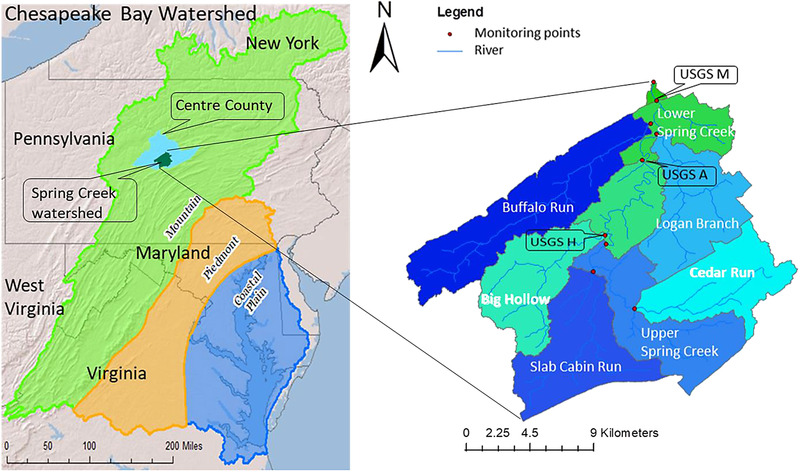
Spring Creek watershed, Centre County, Pennsylvania, USA, showing major subbasins and USGS gauging stations: M = Milesburg, A = Axemann, and H = Houserville. Source: USGS and the Chesapeake Bay Program website (http://www.chesapeakebay.net)
2.2. Model descriptions
2.2.1. The Chesapeake Bay model
The watershed component of the Chesapeake Bay Model was developed to simulate runoff from landscapes upstream of the bay and the associated transport and fate of in‐stream nutrients and sediment that contribute to Chesapeake Bay water quality degradation (CCMP, 2019). Different versions of the model have been operational for more than two decades. Here, we used Phase (5.3) information, which simulates a thousand model segments within the Chesapeake Bay watershed, with an average segment size of 171 km2 and a 21‐yr simulation period. Land‐use categories within the Chesapeake Bay Model include 13 types of cropland, two types of woodland, three types of pasture, and four types of urban land (CCMP, 2019). The model tracks nutrient inputs in manures, fertilizers, and atmospheric deposition on an annual time series, based on a mass balance of county‐level Agricultural Census data such as animal populations, crop yields, area planted, and fertilizer sales.
2.2.2. The Topo‐SWAT model
The SWAT model (Arnold et al., 1998; Neitsch et al., 2011) simulates the impact of changes in land use and management and climate on hydrology and water quality within a watershed (Jeong et al., 2013; Kaini, Artita, & Nicklow, 2012; Veith, Van Liew, Bosch, & Arnold, 2010). Topo‐SWAT, a modified version of the SWAT model that incorporates the topographic wetness index into the input data, can effectively simulate hydrologically active areas, as well as crop growth and agricultural management at the scale of individual fields when detailed data are provided. Topo‐SWAT is therefore capable of capturing temporal and spatial variations in different physicochemical processes resulting from geophysical, management‐related, and climatic differences throughout an agricultural watershed. For the Spring Creek watershed, Amin et al. (2017, 2018) demonstrated the ability of the Topo‐SWAT model to successfully represent karst hydrologic processes and simulate the effects of different conservation dairy cropping scenarios on water and nutrient balances.
2.2.3. Spring Creek baseline setup and validation
Ground‐truthed baseline conditions were represented in Topo‐SWAT, as described by Amin et al. (2017), by incorporating all actual spatial and temporal field‐level details of crop type, crop rotation, and agricultural management practices for each spatially distinct land‐use polygon (i.e., individual agricultural field or set of contiguous, identically managed fields). Each spatially distinct land‐use polygon was further divided by soils, and then into 10 topographic wetness index classes. The intersected results of these layers (land use, soils, topographic index class) form the spatially explicit layer of hydrological response units (HRUs) for the watershed. The HRUs in the wetter topographic index classes indicate the VSAs within the watershed. The HRUs in this project (i.e., Topo‐SWAT's smallest spatial unit) are, thus, smaller than an individual agricultural field (up to several ha), whereas the Chesapeake Bay Model operates on land–river segments (each several hundred km2). Therefore, the Chesapeake Bay Model inputs for the Spring Creek land–river segment supplied, to the extent possible, the inputs and model parameters for the Topo‐SWAT simulations. However, additional details needed for Topo‐SWAT were derived from local information to accurately inform the model's spatial and temporal representation of current agricultural management throughout the watershed. These additional details were found to be consistent, as a whole, with the Chesapeake Bay Model details. In particular, crop types and crop rotations were derived from the cropland data layers of 2008–2014 (USDA, 2015). Farmers’ practices in harvested forage management, such as depth of cut and amount left on field, plus other information on agricultural operations, such as tillage, manure or fertilizer application, cover crop, sowing, harvesting and killing or end of growing season, were collected from the Local Agronomy Guide of Pennsylvania, the USDA National Agricultural Statistics Service (https://www.nass.usda.gov/), stakeholder meetings, and local extension agents.
The Topo‐SWAT model was calibrated and validated for hydrology and water quality at a daily time scale using daily stream flow and bimonthly water quality monitoring data collected at the three USGS gauges obtained from the USGS website (http://waterdata.usgs.gov/pa/nwis/rt), CCMP (2019), and SCWA (2013). A detailed description of input data, model parameters, model assessment, and results of calibration (2002–2007) and validation (2008–2013) of this model can be found in Amin et al. (2017). Values of model performance indicators (R 2, Nash–Sutcliffe efficiencies, and percentage bias) are supplied in the supplemental materials.
2.3. Development and simulation of scenarios
2.3.1. Watershed Implementation Plan (WIP‐2025) scenario
The Chesapeake Bay Program Office provided details and assistance in interpreting the WIP information for the Spring Creek watershed. Accordingly, an updated WIP‐2025 scenario for Spring Creek watershed was developed by shortlisting the official BMP list from the watershed's WIP plan based on expert opinion on local agroecology, locally known information on land use and natural resources, available data and communication with the local farmers, and appropriateness for simulation in the nonpoint source, agriculturally focused Topo‐SWAT model. The Topo‐SWAT WIP‐2025 scenario followed the general WIP guidelines of ranking, design, and implementation hectares for eight BMP categories that are relevant to the Spring Creek watershed and are simulated well in SWAT (Table 1).
TABLE 1.
Description of the best management practices (BMPs) as they were represented in Spring Creek watershed, Centre County, Pennsylvania, using a Topo‐SWAT model with field‐level management data
| BMP category | Description |
|---|---|
| No‐till | No tillage was used on any crop in the multicrop, multiyear rotation, and all crops were planted using no‐till methods. |
| Manure injection | Liquid manure was injected at shallow soil depth. About 90% manure was placed below the top 10‐mm soil layer. A custom‐made mixing device in the Soil and Water Assessment Tool (SWAT) (mixing efficiency = 15%, mixing depth = 100 mm, and random roughness = 10 mm) was added to correctly simulate the manure injection. |
| Spring manure | Manure was applied in the spring instead of fall season. |
| Cover crop | A winter wheat crop was sown at least 2 wk prior to the average frost date without nutrient amendments and was not harvested. |
| 15% less N input | 15% less nitrogen was applied. Nitrogen application rates are often set at, or possibly above, estimated crop requirements to ensure adequate nitrogen availability. |
| Land retirement | Low‐lying croplands were converted to hay or pasture without nutrient amendments. |
| Permanent grass | Croplands were converted to permanent warm‐season grasses without nutrient amendments. |
| Wetland restoration | Agricultural land was reclaimed or converted into wetlands, including forested and nonforested wetlands and emergent marsh. |
| Buffer strip | A 30‐m grassed or forested strip was implemented on each side of the stream. All croplands near hay in the buffer strip area were converted to hay without nutrient, and all croplands near forest were converted to forest. |
The spatially distributed results of nutrient and sediment loss in the baseline Topo‐SWAT scenario were used to identify agriculturally related critical source areas (CSAs), where highly concentrated nutrient source areas and localized hydrologic transport areas (VSAs) coincided in the watershed (Amin et al., 2017). Then, in the Topo‐SWAT WIP‐2025 scenario, BMPs were placed spatially and temporally according to feasibility within the rotation and to vulnerability of the land use to nutrient loss. The land‐use‐altering BMPs were placed first on appropriate land until either no more land was available or the WIP guidelines for implementation quantity of each BMP were met, whichever came first. For example, a 30‐m strip on each side of the stream was recommended for the buffer strip based on the WIP guidelines. About 54% area (732 ha) of the recommended buffer strip was already either grassed or forested (USDA, 2015), so the rest of the area (623 ha) was converted to grass or forest in the simulation. Next, cropland conversion into hay or pasture with no nutrient application was preferentially performed on the cropland most vulnerable to runoff and nutrient loss until the WIP suggested implementation quantity was met. After placing the buffer and other land‐use‐altering BMPs, the management‐related BMPs were applied similarly.
2.3.2. Calculating watershed‐specific best management practice efficiencies for Spring Creek with Topo‐SWAT
The Chesapeake Bay Model uses efficiency based on expert opinion and literature reviews to estimate BMP performance, whereas SWAT primarily simulates BMPs through modification of management processes. To calculate the efficiency of individual BMPs, individualized scenarios were created in Topo‐SWAT in which all study BMPs were singularly applied to all feasible times and places of the baseline scenario. All the scenarios were run for a 10‐yr period. Average N, P, and sediment reduction percentages for the watershed were then calculated from the differences between the BMP and baseline scenario results.
2.3.3. Cost‐effective scenario
Recognizing that final installation costs may vary widely among localities and that some farmers adopt BMPs even without incentive, the final implementation costs per BMP were based on the averages of various literature values. Reported costs ranged from $6.7 to $8.1 ha−1 yr−1 for conservation till or no‐till (Kurkalova, Kling, & Zhao, 2006), −$74 to $34 ha−1 yr−1 (averaging $6.9 ha−1 yr−1) for nutrient management plans (USEPA, 2003a), and $10 to $100 ha−1 yr−1 for cover crops (Mannering, Griffith, & Johnson, 2000; USEPA, 2003b). Land‐use alteration from row crop to permanent grass was estimated to cost $247 ha−1 yr−1 in establishment cost and $250 ha−1 yr−1 in land retirement (Wittenberg & Harsh, 2006). Applying manure via injection can cost 6% more than broadcasting followed by tillage incorporation, and 28% more than broadcast application without incorporation (Hadrich, Harrigan, & Wolf, 2010). Thus, manure injection costs were calculated at $7.5 ha−1 yr−1 when replacing broadcast application with incorporation, and at $29 ha−1 yr−1 when replacing broadcast application without incorporation. Providing sufficient manure storage for farms in this watershed to hold their fall manure application until spring was estimated to cost $0.6 to 0.7 Mg−1 or, on average, $30 ha−1 yr−1 (NRCS, 2015).
Nitrogen has been identified as the priority nutrient needing to be addressed to achieve the TMDL goals for this karst watershed as well as for the Chesapeake Bay (Chesapeake Bay Program, 2019; SCWA, 2013). Thus, to evaluate the lower cost alternative, a cost‐effective ranking of BMPs was performed based on the amount of N load reduction for each monetary unit ($) spent on BMP implementation. Suitable land for implementation of each BMP was identified based on the availability of BMP‐feasible land within each given year of the various cropping rotations. For example, 1980 ha (33% of total cropland) was available to convert into no‐till practices in the watershed in any given year.
A selection of the top most cost‐effective BMPs was then sequentially added to the Topo‐SWAT baseline scenario based on their cost effectiveness rank, as well as the percentage of appropriate land for each BMP that was available, within the top 10% most nutrient‐prone agricultural hectares of the watershed, and then within increasingly less nutrient‐prone agricultural hectares by 10% segments. With each addition of land or BMP, the Topo‐SWAT simulation was rerun and evaluated. This iterative process was continued until the results of the Topo‐SWAT cost‐effective simulation, as compared with the baseline simulation, for N loadings at the Spring Creek watershed outlet showed percentage reductions equal to or greater than those of the bay‐level TMDL goal. The total BMP implementation cost for the watershed was then estimated. Because the BMP rankings, relative differences in cost effectiveness, and implemented areas for this process all vary by watershed and by cost effectiveness goal, the solution for this study will be detailed further in the results section.
3. RESULTS AND DISCUSSION
3.1. Topo‐SWAT model performance for baseline scenario
The ground‐truthed baseline Topo‐SWAT scenario described hydrologic processes in the watershed reasonably well. Specifically, simulated and observed daily streamflow at all three USGS gauging stations of Spring Creek watershed (Milesburg, Axemann, and Houserville; Figure 1) matched for the calibration period of January 2002 to December 2007 and corroboration period of January 2008 to December 2013 (Amin et al., 2017), with daily Nash–Sutcliffe efficiencies of 0.72–0.81 (scale −∞ to 1), percentage bias of 3.5 to −9.8%, and R 2 of .61–.80 (R of .78–.89). Topo‐SWAT predicted that baseflow contributed 83% of the total streamflow during the simulation period, as compared with a baseflow contribution of 87% from measured flow records. A visual comparison of the hydrographs confirmed systematic similarities in timing, duration, and peak height of the majority of storm events. Simulated and observed distributions of water quality variables (N, P, and sediment) were comparable, with a consistently negative percent bias in Topo‐SWAT: −12.9% for N, −9.1% for P, and −4.0% for sediment (Amin et al., 2017). Due to the sparsity of observed water quality data, other model performance indicators were not calculated. However, nutrient and sediment loading rates for individual land‐use types and crop fields were also within ranges of literature values (Amin et al., 2018, 2017). Annual total N, P, and sediment loads for the baseline scenario were 518, 45, and 13,600 Mg yr−1 as predicted by Topo‐SWAT and 570, 42, and 12,900 Mg yr−1 as estimated by the Chesapeake Bay Model (CCMP, 2019).
3.2. Topo‐SWAT simulation of WIP‐2025 scenario
The “15% less N” BMP was the most widely applied BMP in the WIP‐2025 scenario, followed by cover cropping (Table 2). The WIP‐2025 scenario reduced the average annual watershed loadings of N, P, and sediment by 23, 30, and 34%, respectively, as compared with the baseline scenario (Table 2). Thus, the WIP‐2025 scenario simulated in Topo‐SWAT predicted a 2% lower reduction in N than the 25% N reduction target for the Chesapeake Bay‐level TMDL but exceeded both the P and sediment Chesapeake Bay‐level TMDL targets of 24 and 20%, respectively. The WIP‐2025 scenario BMPs, simulated by Topo‐SWAT, were less effective at reducing N loss than at reducing P and sediment loss in the watershed because the major pathways of N loss were leaching (78% of total loss) and subsequent groundwater contribution to the streams. The manure injection BMP used in this scenario was considerably effective at reducing surface runoff losses of N but not subsurface N losses in this karst watershed.
TABLE 2.
Watershed implementation plan (WIP)‐suggested area for the study watershed plus areas, cost involvement, and load reduction, as simulated in Topo‐SWAT, of the best management practices (BMPs) incorporated in the regulatory‐driven, watershed implementation plan scenario, WIP‐2025
| Cumulative load reduction | ||||||
|---|---|---|---|---|---|---|
| WIP suggested area for the watershed | Area of BMP | Cost | Total N | Total P | Sediment | |
| BMPa | ha | ha | US$ | % | ||
| Buffer strip | 695 | 623 | 39,268 | 1.7 | 2.7 | 3.8 |
| Land retirement | 998 | 994 | 297,604 | 7.7 | 18.4 | 17.8 |
| Cover crop | 1,520 | 1,520 | 83,600 | 11.7 | 25.2 | 27.8 |
| No‐till | 261 | 646 | 4,780 | 12.0 | 23.2 | 29.9 |
| Permanent grass | 500 | 315 | 94,311 | 12.5 | 24.5 | 30.8 |
| Wetland restoration | 197 | 181 | 72,219 | 13.8 | 29.0 | 34.6 |
| Manure injection | 97 | 94 | 2,726 | 13.9 | 30.0 | 34.6 |
| 15% less N input | 5,942 | 6,000 | 41,400 | 23.0 | 29.8 | 34.2 |
| Total cost | 635,908 | |||||
Refer to Table 1 for BMP definitions as applied in this study.
Overall, the Topo‐SWAT results are consistent with recent historical water quality trends observed through monitoring in the Spring Creek watershed: P loads in stream discharge have considerably decreased over the last two to three decades, but less so for N, based on the observed nutrient concentration and stream flow data available at http://waterdata.usgs.gov/pa/nwis/rt. Between 2009 and 2017, for the whole Chesapeake Bay watershed, P load was reduced by 21.5% against the target of 15% for this period, whereas N load was only reduced 2.9% as compared with a target of 16% (Chesapeake Bay Program, 2019). Reduction of N loading is clearly proceeding more slowly than the reduction of P in Spring Creek and in the whole Chesapeake Bay watershed, and it is likely the limiting factor in jointly meeting the bay‐level N, P, and sediment TMDLs. Accordingly, the BMPs that were more efficient in N load reduction were identified and incorporated on a priority basis for developing a better management plan, as shown in the sections below.
3.3. Topo‐SWAT estimation of best management practice effectiveness
Each BMP, as predicted by Topo‐SWAT, showed a wide range of impact on nutrient and sediment load reduction and crop yield (Figures 2 and 3), which was expected due to the diversity of soil types, topographic soil wetness classes, land uses, and complex soil–water–plant relationships throughout the watershed. Combined with broadcast manure, no‐till practices reduced denitrification (4.6 kg ha−1, 8.9%), N leaching (1.1 kg ha−1, 8.5%), and soil loss (0.28 Mg ha−1, 16.3%) but increased total N runoff (1.7 kg ha−1, −7.8%) and total P loss (3.0 kg ha−1, −38.1%) because of less manure incorporation into the soil. The results agree with the findings of Garcia, Veith, Kleinman, Rotz, and Saporito (2008) and Wilson, Dalzell, Mulla, Dogwiler, and Porter (2014) showing that lack of manure incorporation with no‐till enhanced total P loss (0.43 kg ha−1 in clay loam soil) but reduced soil loss. Compared with manure incorporation, surface manure application without tillage typically increases losses of ammonia N through volatilization (Nathan & Malzer, 1994), and this likely reduces manure N available for other N‐loss pathways such as leaching and denitrification (Velthof, Kuikman, & Oenema, 2003). Decreased soil erosion under no‐till limited the sediment‐bound transport of nutrients, as also reported by Legge et al. (2013), but the absence of tillage and associated incorporation increased surface loss of manure constituents during subsequent storm events.
FIGURE 2.
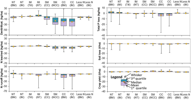
Changes in nutrient (N and P) losses, sediment (soil) loss, and crop yield (note different scales in the graph) by different efficiency‐type best management practices (BMPs) in Spring Creek watershed, Centre County, Pennsylvania. Dotted lines indicate‐no change (zero) lines, NT = no‐till, BM = broadcast manure, IM = injected manure, SM = spring applied manure, CC = cover crop, NCC = no cover crop, less N = 15% less N input (BMP descriptions in Table 1)
FIGURE 3.
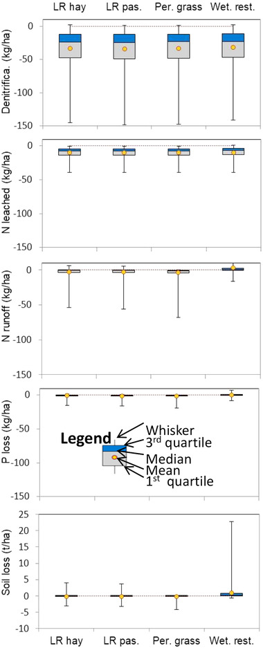
Changes in nutrient (N and P) losses, sediment (soil) loss, and crop yield by different land‐use‐altering best management practices (BMPs) in Spring Creek watershed, Centre County, Pennsylvania. Dotted lines indicate no‐change (zero) lines, LR hay = land retirement into hay, LR pas. = land retirement into pasture, Per. grass = permanent grass, Wet. rest. = wetland restoration (BMP descriptions in Table 1)
In contrast, when combined with manure injection, no‐till reduced denitrification less (0.68 kg ha−1), reduced N runoff more (4.7 kg ha−1), and increased P loss less (1.4 kg ha−1) than broadcast manure application. The reported effectiveness of no‐till practices and conservation tillage varies substantially. For example, Folle, Dalzell, and Mulla (2007) found that conservation tillage reduced P loss by 15–25%, but that P loss range expands to 10–95% in a comprehensive literature review by Gitau, Gburek, and Jarret (2005) of northeastern US studies. Douglas‐Mankin, Daggupati, Sheshukov, and Barnes (2013) observed soil loss reduction by 58–83% due to no‐till. The overall effectiveness of no‐till management in reducing overland pollutant losses in the Spring Creek watershed is diminished, as compared with areas dominated by overland‐flow hydrology, because the karst hydrology is dominated by minimal surface runoff and high infiltration (Taylor, 1997).
Subsurface injection of liquid manure also reduced N volatilization (90%) and surface runoff‐mediated nutrient losses (6.7 kg N ha−1 and 1.05 kg P ha−1) (Figure 2). The effectiveness of this practice is dependent on the technology used for injection. Manure injection with conventional tillage offered minimal environmental benefit compared with injection with no‐till (Figure 2). Because conventional tillage after manure broadcasting incorporates manure into the soil, injection does not provide considerable additional benefit over broadcasting immediately before conventional tillage. Disturbance due to injection can slightly increase the erosion risks, but the subsurface injection also impedes the runoff loss of nutrients (Jahanzad, Saporito, Karsten, & Kleinman, 2019). Average reductions of N runoff (0.1 kg ha−1, 0.5%) and P loss (0.2 kg ha−1, 3.6%), and average increases of N leaching (0.1 kg ha−1) were predicted in this study. In contrast, manure injection was much more effective with no‐till management, reducing both N runoff (7.8 kg ha−1, 36.1%) and P loss (1.24 kg ha−1, 15.6%) and increasing crop yield (0.17 Mg ha−1). Disturbance during manure injection increased soil loss (0.04 Mg ha−1). Decreased runoff loss enhanced nutrient availability in the root zone and thus increased crop yield. Some of the persisting N in soil was subsequently denitrified or leached, so the manure injection resulted in more N leaching (8.0%) and denitrification (8.1%) as compared with broadcast manure. Amin et al. (2013) observed statistically insignificant changes in N leaching for manure injection under similar weather conditions. In the Spring Creek watershed, Jahanzad et al. (2019) compared manure injection and surface broadcast over 4 yr, and although P losses were variable and did not differ in 3 yr, P accumulated over time, and when P losses in runoff were greatest, manure injection reduced total P loss by 60% compared with surface broadcast application.
In the current study area, manure was usually applied either in spring or fall. When combined with cover crops, broadcast spring manure application was found beneficial over the broadcast fall application. Broadcast spring manure application reduced N runoff (0.7 kg ha−1), N leaching (5.5 kg ha−1), denitrification (18.0 kg ha−1), P loss (0.4 kg ha−1), and soil loss (0.18 Mg ha−1) compared with fall manure application. The crop yield was also larger (36.6%) with spring application because the nutrients of fall‐applied manure partly diminished before the following spring crop. The benefit of spring manure application over fall application was 83% less for N leaching and 13% less for P loss (Figure 2) when the cover crop was incorporated because nutrients consumed by the cover crop became unavailable for loss, and the cover crop vegetation reduced erosion. Cover cropping was the most effective efficiency‐type BMP regardless of manure application method (Figure 2). With manure injection, cover cropping reduced N runoff (6.1 kg ha−1, 44.1%), N leaching (6.1 kg ha−1, 43.7%), denitrification (22.3 kg ha−1, 39.8%), P loss (3.1 kg ha−1, 46.1%), and soil loss (1.05 Mg ha−1, 63.2%). Cover cropping has proven its effectiveness in controlling nonpoint‐source pollution across a wide range of watersheds. In a midwestern watershed, Hanrahan et al. (2018) quantified 69–90% less nitrate N loss in tile drains from fields planted to cover crops than from fields without cover crops. Further, in a meta‐analysis of 77 N leachate studies, Tonitto, David, and Drinkwater (2006) found that nonlegume cover crops reduced N leaching, on average, by 70% relative to bare fallow, without negative impacts on the subsequent crop, and legume cover crops reduced nitrate leaching by 40% relative to bare fallow. Arabi et al. (2008) observed that cover crops reduced N, P, and sediment loading by 14, 10, and 3%, respectively. Folle et al. (2007) found 16% N and 29% P loss reduction by introducing rye (Secale cereale L.) cover crop.
In the current study, adopting cover crops also increased average crop yield by 18.9 and 17.6% under broadcast and injected manure, respectively. A 65‐study meta‐analysis of corn yield response to cover crops across the United States found that legume cover crops increased corn yields by 30–33% (Marcillo & Miguez, 2017). When fall‐applied manure was combined with rye cover crop in a 2‐yr field study in the Spring Creek watershed, Milliron, Karsten, and Beegle (2019) found that corn yields following a rye cover crop were 23% greater after injected manure than after broadcast manure.
Application of 15% less N reduced N loss in all pathways as expected, including N in runoff (0.3 kg ha−1, 2.1%), leaching (1.2 kg ha−1, 8.3%), and denitrification (3.9 kg ha−1, 7.6%). However, total P (0.05 kg ha−1, 0.8%) and sediment load (0.02 Mg ha−1) increased slightly. Applying 15% less N also reduced average crop yield by 8.0–9.2%. The associated reductions in biomass production and vegetative coverage might have accounted for increases in soil erosion and sediment‐bound P transport. Indeed, Folle et al. (2007) reported that 20% less N application in fall reduced N loss by 20%, whereas the same N rate reduction in spring caused only a 6.8% reduction in N loss. Notably, 34% less P application reduced total P loss by ∼28%. Cerro et al. (2014) stated that 20% less fertilizer application reduced N leaching by 34% and yield by 3%.
Land‐use‐altering BMPs were nearly all equally effective for reducing nutrient loss (Figure 3), as modeled in Topo‐SWAT. Land retirement as hay or pasture without nutrient application and establishing perennial orchard grass reduced N runoff (6.6 kg ha−1, 85.5%), N leaching (6.2 kg ha−1, 79.5%), and denitrification (26.1 kg ha−1, 77.3%). These land‐use‐altering BMPs also reduced P loss by 3.4 kg ha−1 (92.7%) and soil loss by 0.53 Mg ha−1 (87.6%). The predictions are in agreement with the findings of Wilson et al. (2014), who obtained >85% reduction of P and sediment loss by changing land use from row crop to pasture in a karst watershed. Restored wetland, via conversion of cropland to forested wetland, had much lower N leaching and denitrification than cropland. It was unexpected that restoring wetlands would increase soil loss. This finding may be due to limitations in how SWAT was used to simulate wetlands. However, the scenario results were not affected by any minor error in simulating soil loss from wetlands, since effectiveness in soil loss reduction was not considered when ranking the BMPs for N reduction, and since the wetland restoration BMP was determined too costly to be used in the Topo‐SWAT cost‐effective scenario for this study. Grassed and forested buffer strips reduced both nutrient (13.9 kg N ha−1 and 3.36 kg P ha−1) and sediment (0.82 Mg ha−1) loss substantially.
3.4. Topo‐SWAT estimation of best management practice cost effectiveness
No‐till ranked highest among the BMPs studied based on cost effectiveness of N loss reduction (0.83 kg $−1) (Table 3). Cost effectiveness among manure injection, cover crop, grass buffer strip, and 15% less N input was similar (0.21–0.23 kg $−1) and about four times less than for no‐till. Similar results were obtained by Kieser & Associates (2008) who found no‐till as the most cost‐effective (1.47 kg $−1) BMP to reduce N loss in the Paw Paw River watershed in Michigan. The cost effectiveness ranking of the other BMPs they studied was as follows: combination of edge‐of‐field filter strips and no‐till (0.45 kg $−1) > edge‐of‐field filter strip (0.41 kg $−1) > rye cover crop (0.30 kg $−1) > 25% less fertilizer application (0.08 kg $−1). The ranking of BMPs in Kansas was no‐till (1.2 kg $−1) > buffers and vegetative filters (0.91 kg $−1) > cover crop (0.32–0.8 kg $−1), and 32% less N rate was slightly more cost effective than avoiding fall N application (Wortmann et al., 2011). There are ranking similarities in those studies, but the cost effectiveness varied across farming systems, environmental conditions, and time. Liu et al. (2014) obtained higher cost–benefit ratio of no‐till (114%) compared with fertilizer management (96 and 89%) for reducing nutrient load in a large tributary of the Three Gorges Reservoir in China. Ahmadi et al. (2015) found fertilizer management more effective than grassed waterways and tillage management for nitrate load reduction in the Eagle Creek watershed, Indiana.
TABLE 3.
Estimated watershed average cost effectiveness of the best management practices (BMPs) in reducing nutrient and sediment loads in Spring Creek watershed
| Load reduction | ||||||
|---|---|---|---|---|---|---|
| N loss | P loss | Soil loss | BMP application cost | N loss reduction per unit cost | ||
| BMPa | kg ha−1 yr−1 | kg ha−1 yr−1 | Mg ha−1 yr−1 | US$ ha−1 yr−1 | kg US$−1 | N‐based BMP rank |
| No‐till | 6.2 | −1.62 | 0.31 | 7.4 | 0.83 | 1 |
| Manure injection | 6.8 | 1.24 | 0.04 | 29 | 0.23 | 2 |
| Cover crop | 12.2 | 3.10 | 1.05 | 55 | 0.22 | 3 |
| Grass buffer | 13.9 | 3.36 | 0.82 | 63 | 0.22 | 4 |
| 15% less N input | 1.4 | −0.05 | −0.02 | 6.9 | 0.21 | 5 |
| Land retirement | 12.8 | 3.36 | 0.53 | 299 | 0.04 | 6 |
| Spring manure | 0.8 | 0.35 | 0.00 | 30 | 0.03 | 7 |
| Wetland restoration | 6.6 | 0.41 | 0.00 | 392 | 0.02 | 8 |
Refer to Table 1 for BMP definitions as applied in this study.
In the current study, N‐reduction cost effectiveness of land retirement and wetland restoration (0.02 and 0.04 kg $−1, respectively) was negligible due to the BMPs’ relatively large implementation costs (Table 3). On the other hand, the low cost effectiveness (0.03 kg $−1) of spring manure application was attributed to its low performance in N loss reduction. Cost effectiveness of a BMP also varies with the scale of implementation; for example, large‐scale filter strip installation can diminish its cost effectiveness (Kieser & Associates, 2008). Similar BMP cost effectiveness rankings can be conducted for other watersheds in the upper Chesapeake Bay region.
3.5. Topo‐SWAT simulation of cost‐effective scenario
Results from the N‐based cost effectiveness ranking in the previous section show that no‐till was four times more cost effective than any other BMP considered in this watershed. Thus, no‐till implementation was prioritized on all appropriate land when creating the Topo‐SWAT cost‐effective scenario from the Topo‐SWAT baseline. Second, the next four highest‐ranked BMPs (cover cropping, manure injection, 15% less N input, and grass buffer), which were ranked almost equally cost effective in reducing N, were added as a group to the 10% most nutrient‐loss‐prone fields within the Topo‐SWAT cost‐effective scenario and evaluated. As with the Topo‐SWAT WIP‐2025 scenario, the Topo‐SWAT cost‐effective scenario was updated and reevaluated iteratively as the allowable hectares for implementation gradually were increased. The process continued until the percentage reduction in N at the Spring Creek watershed outlet, as simulated in Topo‐SWAT, equaled the bay‐level TMDL goal for N loadings into the bay.
Ultimately, for the Spring Creek watershed, Topo‐SWAT simulations required implementation of no‐till, manure injection, cover crop, grass buffer, and 15% less N input in all suitable agricultural land to achieve the same level of reduction in N loadings at the watershed outlet as the bay‐level TMDL goal (Table 4). The final Topo‐SWAT cost‐effectiveness scenario resulted in implementing no‐till and cover cropping on three times more hectares than in the Topo‐SWAT WIP‐2025 scenario. However, these BMPs can help reduce denitrification, increase soil health by retaining organic matter to slowly degrade on the field, and enhance plant uptake of nutrients.
TABLE 4.
Areas, cost involvement, and load reduction, as simulated in Topo‐SWAT, of the best management practices (BMPs) incorporated in the cost‐effective scenario based on N as a limiting factor
| Cumulative load reduction | |||||
|---|---|---|---|---|---|
| BMP area | Cost | Total N | Total P | Sediment | |
| BMPa | ha | US$ | % | ||
| No‐till | 1,980 | 14,652 | 3 | −5 | 4 |
| Manure injection | 6,000 | 174,000 | 11 | 6 | 6 |
| Cover crop | 4,200 | 231,000 | 22 | 26 | 34 |
| Grass buffer | 176 | 11,097 | 23 | 27 | 35 |
| 15% less N input | 6,000 | 41,400 | 25 | 26 | 34 |
| Total cost | 472,149 | ||||
Refer to Table 1 for BMP definitions as applied in this study.
Both simulation scenarios essentially met the bay‐level TMDL goals for N, P, and sediment using only a portion of the BMPs suggestion on the WIP guidelines for the watershed. The Topo‐SWAT cost‐effective scenario we identified reduced N and P loads almost equally (25 and 26%, respectively) and sediment by 34%, whereas the Topo‐SWAT WIP‐2025 scenario reduced N and P by 23 and 30%, respectively, and sediment by 34%. Both scenarios reduced N loss elsewhere in the N cycle, such as denitrification, volatilization, and leaching. However, total implementation costs for the Topo‐SWAT cost‐effective scenario were 26% less than for the Topo‐SWAT WIP‐2025 scenario because the cost‐effective scenario requires the most cost‐effective BMPs to be implemented first. By design, the cost‐effective scenario spreads costs for BMP implementation throughout the watershed at smaller amounts per person than scenarios that incorporate larger‐cost restoration‐type BMPs.
It is important to note that BMP performance uncertainty can be intensified in extreme climate scenarios (Woznicki & Nejadhashemi, 2014), and possible impacts of climate change on the processes simulated in the study need to be investigated. Average ambient temperatures in the region are projected to increase by 3°C by 2050 (Karmalkar & Bradley, 2017), and the number of heavy precipitation and extreme runoff events is expected to increase as climate change continues to accelerate (IPCC, 2014). Agronomic management practices may need to be altered to offset the climate change impacts (Prasad et al., 2018).
4. CONCLUSIONS
We leveraged the fine‐resolution temporal and spatial capabilities of Topo‐SWAT to inform localized selection and placement of the agricultural BMPs that had been specified as necessary, within the Pennsylvania WIP for Spring Creek watershed, in order for all watersheds in Pennsylvania to jointly meet Pennsylvania's portion of the Chesapeake Bay TMDL goals for N, P, and sediment. Working from a baseline Topo‐SWAT simulation that is representative of current land management practices, WIP‐suggested BMPs were individually simulated throughout the watershed. Average annual BMP pollution reduction efficiencies and cost‐effectiveness values were calculated. Best management practices were ranked based on cost effectiveness in reducing N load, which has been determined limiting factor toward fully meeting the bay‐level TMDL goals for N, P, and sediment. Individual BMP cost effectiveness for reducing nutrient and sediment loading varied, with no‐till ranking the most cost effective and implementation‐intensive BMPs such as wetland restoration ranking the least cost effective. Topo‐SWAT simulations of two scenarios with the WIP‐suggested BMPs were evaluated. These scenarios were derived from the Topo‐SWAT baseline scenario based on (i) WIP implementation guidelines for quantities of BMP hectares within Spring Creek, and (ii) selection of the most cost‐effective BMPs for reducing N loadings to the streams. Both scenarios nearly met or exceeded, at the watershed outlet, the bay‐level TMDL target load reductions for N, P, and sediment entering the bay. The WIP‐2025 Topo‐SWAT simulation implemented only eight major categories of BMPs listed in the Spring Creek WIP, whereas the Topo‐SWAT cost‐effective model implemented even fewer BMPs and with 26% less cost, but on more land. By incorporating fine‐resolution spatial data and modeling the region's VSA hydrology, Topo‐SWAT identified high‐risk, nutrient transport areas. By additionally using localized field‐level management data for the agricultural cropping rotations, Topo‐SWAT highlighted agricultural fields within CSAs for nutrient and sediment mitigation. Regional‐level modeling, such as the Chesapeake Bay watershed model, can provide general BMP suggestions for land–river segment watersheds, which are the Chesapeake Bay model's smallest spatial unit. The use of Topo‐SWAT to simulate the land–river segment watershed at a much finer resolution, as done in this study, can then provide a localized selection and placement of WIP‐suggested and other BMPs that jointly achieve the same or greater pollution reduction at a lower cost. The resulting scenario contributes to a more locally relevant, cost‐effective scenario than the TMDL‐derived regulatory WIP scenario and, in doing so, encourages and supports local involvement and stewardship.
CONFLICT OF INTEREST
The authors declare no conflict of interest.
Supporting information
Supplemental Fig. S1. Land cover map of Spring Creek watershed. (Source: Amin et al., 2017)
Supplemental Fig. S2. Simulated and observed daily streamflow at USGS guaging stations (Milesburg, Axemann, and Houserville) of Spring Creek watershed for a calibration period of Jan 2002–Dec 2007 and validation period of Jan 2008–Dec 2013.
Supplemental Fig. S3. Simulated (number of data points = 2920) and observed (number of observations = 57) sediment, total nitrogen (N), and total phosphorous (P) concentration at USGS Axemann gage station of Spring Creek watershed for the period of 2000–2008 (Solid circles in the figure indicate mean value).
Supplemental Fig. S4. Nutrient and sediment loadings from Spring Creek watershed outlet as estimated from the observations by the Chesapeake Bay Program (CCMP, 2015) and the Topo‐SWAT model.
Supplemental Table S1 Eight crop rotations incorporated in SWAT model to represent the annual crop cover over the watershed.
Supplemental Table S2 Performance indicators of SWAT streamflow predictions of Spring Creek watershed (Source: Amin et al., 2017).
ACKNOWLEDGMENTS
This publication was developed under USEPA Assistance Agreement RD 83556801‐0. It has not been formally reviewed by the USEPA. We also acknowledge support from the Department of Plant Science, Pennsylvania State University, and the USDA‐ARS Pasture Systems and Watershed Management Research Unit. We are grateful to the Chesapeake Community Modeling Program, particularly Gary Shenk and Jeff Sweeney, for assistance interpreting Chesapeake Bay Model inputs and outputs. Mention of trade names or commercial products is solely for providing specific information and does not imply recommendation or endorsement by the USDA, USEPA, or Pennsylvania State University. All entities involved are equal opportunity providers and employers.
Amin MGM, Veith TL, Shortle JS, Karsten HD, Kleinman PJA. Addressing the spatial disconnect between national‐scale total maximum daily loads and localized land management decisions. J. Environ. Qual 2020;49:613–627. 10.1002/jeq2.20051
Assigned to Associate Editor Anthony Buda.
REFERENCES
- Ahmadi, M. , Arabi, M. , Fontane, D. , & Engel, B. (2015). Application of multicriteria decision analysis with a priori knowledge to identify optimal nonpoint source pollution control plans. Journal of Water Resources Planning and Management, 141, 04014054 10.1061/(ASCE)WR.1943-5452.0000455 [DOI] [Google Scholar]
- Amin, M. G. M. , Forslund, A. , Bui, X. Z. , Juhler, R. K. , Petersen, S. O. , & Lægdsmand, M. (2013). Persistence and leaching potential of microorganisms and mineral N in animal manure applied to intact soil columns. Applied and Environmental Microbiology, 79, 535–542. 10.1128/AEM.02506-12 [DOI] [PMC free article] [PubMed] [Google Scholar]
- Amin, M. G. M. , Karsten, H. D. , Veith, T. L. , Beegle, D. B. , & Kleinman, P. J. A. (2018). Conservation dairy farming impact on water quality in a karst watershed in northeastern US. Agricultural Systems, 165, 187–196. 10.1016/j.agsy.2018.06.010 [DOI] [Google Scholar]
- Amin, M. G. M. , Veith, T. L. , Collick, A. S. , Karsten, H. D. , & Buda, A. R. (2017). Simulating hydrological and nonpoint source pollution processes in a karst watershed: A variable source area hydrology model evaluation. Agricultural Water Management, 180, 212–223. 10.1016/j.agwat.2016.07.011 [DOI] [Google Scholar]
- Arabi, M. , Frankenberger, J. R. , Engel, B. A. , & Arnold, J. G. (2008). Representation of agricultural conservation practices with SWAT. Hydrological Processes, 22, 3042–3055. 10.1002/hyp.6890 [DOI] [Google Scholar]
- Arnold, J. G. , Srinivasan, R. , Muttiah, R. S. , & Williams, J. R. (1998). Large area hydrologic modeling and assessment. Part I: Model development. Journal of the American Water Resources Association, 34, 73–89. 10.1111/j.1752-1688.1998.tb05961.x [DOI] [Google Scholar]
- Bechmann, M. E. , Kleinman, P. J. A. , Sharpley, A. N. , & Saporito, L. S. (2005). Freeze–thaw effects on phosphorus loss in runoff from manured and catch‐cropped soils. Journal of Environmental Quality, 34, 2301–2309. 10.2134/jeq2004.0415 [DOI] [PubMed] [Google Scholar]
- Beven, K. J. , & Kirkby, M. J. (1979). A physically‐based, variable contributing area model of basin hydrology. Hydrological Sciences Bulletin, 24, 43–69. 10.1080/02626667909491834 [DOI] [Google Scholar]
- Brooks, R. P. , Yetter, S. E. , Carline, R. F. , Shortle, J. S. , Bishop, J. A. , Ingram, H. , … Piechnik, D. (2011). Analysis of BMP implementation performance and maintenance in Spring Creek, an agriculturally‐influenced watershed in Pennsylvania (Final Report). Washington, DC: USDA CEAP. [Google Scholar]
- Buda, A. R. , & DeWalle, D. R. (2009). Dynamics of stream nitrate sources and flow pathways during storm flows on urban, forest and agricultural watersheds in central Pennsylvania, USA. Hydrological Processes, 23, 3292–3305. 10.1002/hyp.7423 [DOI] [Google Scholar]
- Buda, A. R. , Kleinman, P. J. A. , Srinivasan, M. S. , Bryant, R. B. , & Feyereisen, G. W. (2009). Effects of hydrology and field management on phosphorus transport in surface runoff. Journal of Environmental Quality, 38, 2273–2284. 10.2134/jeq2008.0501 [DOI] [PubMed] [Google Scholar]
- Chesapeake Bay Program . (2018a). Chesapeake Bay Program partnership exceeds 2017 targets for reducing phosphorus, sediment pollution . Retrieved from https://www.chesapeakebay.net/images/press_release_pdf/CBP_Media_Release_Reducing_Pollution_FINAL.pdf
- Chesapeake Bay Program . (2018b). Phase III WIP planning targets . Retrieved from https://www.chesapeakebay.net/documents/Phase_III_WIP_Planning_Targets.pdf
- Chesapeake Bay Program . (2019). Chesapeake progress: 2017 and 2025 watershed implementation plans (WIPs) . Retrieved from http://www.chesapeakeprogress.com/clean-water/water-quality/watershed-implementation-plans
- CCMP (Chesapeake Community Modeling Program) . (2019). CCMP navigation: Models & data . Retrieved from http://ches.communitymodeling.org/models/CBPhase5/index.php
- Cerro, I. , Antiguedad, I. , Srinivasan, R. , Sauvage, S. , Volk, M. , & Sanchez‐Perez, J. M. (2014). Simulating land management options to reduce nitrate pollution in an agricultural watershed dominated by an alluvial aquifer. Journal of Environmental Quality, 43, 67–74. 10.2134/jeq2011.0393 [DOI] [PubMed] [Google Scholar]
- Collick, A. S. , Fuka, D. R. , Kleinman, P. J. A. , Buda, A. R. , Weld, J. L. , White, M. J. , … Easton, Z. M. (2015). Predicting phosphorus dynamics in complex terrains using a variable source area hydrology model. Hydrological Processes, 29, 588–601. 10.1002/hyp.10178 [DOI] [Google Scholar]
- Douglas‐Mankin, K. R. , Daggupati, P. , Sheshukov, A. Y. , & Barnes, P. L. (2013). Paying for sediment: Field‐scale conservation practice targeting, funding, and assessment using the Soil and Water Assessment Tool. Journal of Soil and Water Conservation, 68, 41–51. 10.2489/jswc.68.1.41 [DOI] [Google Scholar]
- Easton, Z. M. , Fuka, D. R. , Walter, M. T. , Cowan, D. M. , Schneiderman, E. M. , & Steenhuis, T. S. (2008a). Re‐conceptualizing the Soil and Water Assessment Tool (SWAT) model to predict runoff from variable source areas. Journal of Hydrology, 348, 279–291. 10.1016/j.jhydrol.2007.10.008 [DOI] [Google Scholar]
- Easton, Z. M. , Walter, M. T. , & Steenhuis, T. S. (2008b). Combined monitoring and modeling indicate the most effective agricultural best management practices. Journal of Environmental Quality, 37, 1798–1809. 10.2134/jeq2007.0522 [DOI] [PubMed] [Google Scholar]
- Folle, S. , Dalzell, B. , & Mulla, D. (2007). Evaluation of best management practices (BMPs) in impaired watersheds using the SWAT model. St. Paul: University of Minnesota. [Google Scholar]
- Fulton, J. W. , Koerkle, E. H. , McAuley, S. D. , Hoffman, S. A. , & Zarr, L. F. (2005). Hydrogeologic setting and conceptual hydrologic model of the Spring Creek basin, Centre County, Pennsylvania (Scientific Investigations Report 2005‐5091). Reston, VA: USGS. [Google Scholar]
- Garcia, A. M. , Veith, T. L. , Kleinman, P. J. A. , Rotz, C. A. , & Saporito, L. S. (2008). Assessing manure management strategies through small‐plot research and whole‐farm modeling. Journal of Soil and Water Conservation, 63, 204–211. 10.2489/jswc.63.4.204 [DOI] [Google Scholar]
- Ghebremichael, L. T. , Veith, T. L. , & Hamlett, J. M. (2013). Integrated watershed‐ and farm‐scale modeling framework for targeting critical source areas while maintaining farm economic viability. Journal of Environmental Management, 114, 381–394. 10.1016/j.jenvman.2012.10.034 [DOI] [PubMed] [Google Scholar]
- Ghebremichael, L. T. , Veith, T. L. , & Watzin, M. C. (2010). Determination of critical source areas for phosphorus loss: Lake Champlain basin, Vermont. Transactions of the ASABE, 53, 1595–1604. 10.13031/2013.34898 [DOI] [Google Scholar]
- Giri, S. , Nejadhashemi, A. P. , Woznicki, S. A. , & Zhang, Z. (2014). Analysis of best management practice effectiveness and spatiotemporal variability based on different targeting strategies. Hydrological Processes, 28, 431–445. 10.1002/hyp.9577 [DOI] [Google Scholar]
- Gitau, M. W. , Gburek, W. J. , & Jarret, A. R. (2005). A tool for estimating best management practice effectiveness for phosphorus pollution control. Journal of Soil and Water Conservation, 60, 1–10. [Google Scholar]
- Gitau, M. W. , Veith, T. L. , Gburek, W. J. , & Jarrett, A. R. (2006). Watershed‐level best management practice selection and placement in the Town Brook watershed, New York. Journal of the American Water Resources Association, 42, 1565–1581. 10.1111/j.1752-1688.2006.tb06021.x [DOI] [Google Scholar]
- Hadrich, J. C. , Harrigan, T. M. , & Wolf, C. A. (2010). Economic comparison of liquid manure transport and land application. Applied Engineering in Agriculture, 26, 743–758. 10.13031/2013.34939 [DOI] [Google Scholar]
- Hanrahan, B. R. , Tank, J. L. , Christopher, S. F. , Mahl, U. H. , Trentman, M. T. , & Royer, T. V. (2018). Winter cover crops reduce nitrate loss in an agricultural watershed in the central U.S. Agriculture, Ecosystems & Environment, 265, 513–523. 10.1016/j.agee.2018.07.004 [DOI] [Google Scholar]
- IPCC . (2014). IPCC summary for policymakers In Pachauri R. K., & Meyer L. A. (Eds.), Climate change 2014 synthesis report: Contribution of Working Groups I, II and III to the Fifth Assessment Report of the Intergovernmental Panel on Climate Change (pp. 2–26). Geneva: IPCC. [Google Scholar]
- Jahanzad, E. , Saporito, L. S. , Karsten, H. D. , & Kleinman, P. J. A. (2019). Varying influence of dairy manure injection on phosphorus loss in runoff over four years. Journal of Environmental Quality, 48, 450–458. 10.2134/jeq2018.05.0206 [DOI] [PubMed] [Google Scholar]
- Jeong, J. , Kannan, N. , Arnold, J. , Glick, R. , Gosselink, L. , Srinivasan, R. , & Barrett, M. (2013). Modeling sedimentation‐filtration basins for urban watersheds using Soil and Water Assessment Tool. Journal of Environmental Engineering, 139, 838–848. 10.1061/(ASCE)EE.1943-7870.0000691 [DOI] [Google Scholar]
- Kaini, P. , Artita, K. , & Nicklow, J. (2012). Optimizing structural best management practices using SWAT and genetic algorithm to improve water quality goals. Water Resources Management, 26, 1827–1845. [Google Scholar]
- Karmalkar, A. V. , & Bradley, R. S. (2017). Consequences of global warming of 1.5°C and 2°C for regional temperature and precipitation changes in the contiguous United States. PLOS ONE, 12, e0168697 10.1371/journal.pone.0168697 [DOI] [PMC free article] [PubMed] [Google Scholar]
- Kieser & Associates . (2008). Modeling of agricultural BMP scenarios in the Paw Paw River watershed using the Soil and Water Assessment Tool (SWAT) . Retrieved from http://kieser-associates.com/uploaded/pawpaw_swat_modeling_report_final_v4.pdf
- Kleinman, P. J. A. , Sharpley, A. N. , McDowell, R. W. , Flaten, D. , Buda, A. R. , Tao, L. , … Zhu, Q. (2011). Managing agricultural phosphorus for water quality protection: Principles for progress. Plant and Soil, 349, 169–182. 10.1007/s11104-011-0832-9 [DOI] [Google Scholar]
- Kurkalova, L. , Kling, C. , & Zhao, J. (2006). Green subsidies in agriculture: Estimating the adoption costs of conservation tillage from observed behavior. Canadian Journal of Agricultural Economics, 54, 247–267. 10.1111/j.1744-7976.2006.00048.x [DOI] [Google Scholar]
- Legge, J. T. , Doran, P. J. , Herbert, M. E. , Asher, J. , O'Neil, G. , Mysorekar, S. , … Hall, K. R. (2013). From model outputs to conservation action: Prioritizing locations for implementing agricultural best management practices in a midwestern watershed. Journal of Soil and Water Conservation, 68, 22–33. 10.2489/jswc.68.1.22 [DOI] [Google Scholar]
- Liu, R. , Zhang, P. , Wang, X. , Wang, J. , Yu, W. , & Shen, Z. (2014). Cost‐effectiveness and cost‐benefit analysis of BMPs in controlling agricultural nonpoint source pollution in China based on the SWAT model. Environmental Monitoring and Assessment, 186, 9011–9022. 10.1007/s10661-014-4061-6 [DOI] [PubMed] [Google Scholar]
- Mannering, J. V. , Griffith, D. R. , & Johnson, K. D. (2000). Winter cover crops: Their value and management . Purdue University. Retrieved from http://www.browncountyswcd.com/wp-content/uploads/2018/06/winter-cover-crops.pdf
- Marcillo, G. S. , & Miguez, F. E. (2017). Corn yield response to winter cover crops: An updated meta‐analysis. Journal of Soil and Water Conservation, 72, 226–239. 10.2489/jswc.72.3.226 [DOI] [Google Scholar]
- Milliron, R. A. , Karsten, H. D. , & Beegle, D. B. (2019). Influence of dairy slurry manure application method, fall application‐timing, and winter rye management on nitrogen conservation. Agronomy Journal, 111, 995–1009. 10.2134/agronj2017.12.0743 [DOI] [Google Scholar]
- Nathan, M. V. , & Malzer, G. L. (1994). Dynamics of ammonia volatilization from turkey manure and urea applied to soil. Soil Science Society of America Journal, 58, 985–990. 10.2136/sssaj1994.03615995005800030050x [DOI] [Google Scholar]
- Neitsch, S. L. , Arnold, J. G. , Kiniry, J. R. , & Williams, J. R. (2011). Soil and Water Assessment Tool theoretical documentation, version 2009. College Station: Texas A&M University System. [Google Scholar]
- NRCS . (2015). Costs associated with development and implementation of comprehensive nutrient management plans Part I: Nutrient management, land treatment, manure and wastewater handling and storage, and recordkeeping. USDA‐NRCS; Retrieved from https://www.nrcs.usda.gov/Internet/FSE_DOCUMENTS/nrcs143_012131.pdf [Google Scholar]
- O'Driscoll, M. A. , & DeWalle, D. R. (2006). Stream‐air temperature relations to classify stream‐ground water interactions in a karst setting, central Pennsylvania, USA. Journal of Hydrology, 329, 140–153. 10.1016/j.jhydrol.2006.02.010 [DOI] [Google Scholar]
- Panagopoulos, Y. , Makropoulos, C. , & Mimikou, M. (2012). Decision support for diffuse pollution management. Environmental Modelling & Software, 30, 57–70. 10.1016/j.envsoft.2011.11.006 [DOI] [Google Scholar]
- Piechnik, D. A. , Goslee, S. C. , Veith, T. L. , Bishop, J. A. , & Brooks, R. P. (2012). Topographic placement of management practices in riparian zones to reduce water quality impacts from pastures. Landscape Ecology, 27, 1307–1319. 10.1007/s10980-012-9783-7 [DOI] [Google Scholar]
- Prasad, R. , Gunn, S. K. , Rotz, C. A. , Karsten, H. D. , Roth, G. , Buda, A. , & Stoner, A. M. K. (2018). Projected climate and agronomic implications for corn production in the northeastern United States. PLOS ONE, 3, e0198623 10.1371/journal.pone.0198623 [DOI] [PMC free article] [PubMed] [Google Scholar]
- PSC . (2015). Pennsylvania State Climatologist homepage. Retrieved from http://climate.psu.edu
- Rabotyagov, S. , Campbell, T. , Jha, M. , Gassman, P. , Arnold, J. , Kurkalova, L. , … Kling, C. L. (2010). Least‐cost control of agricultural nutrient contributions to the Gulf of Mexico hypoxic zone. Ecological Applications, 20, 1542–1555. 10.1890/08-0680.1 [DOI] [PubMed] [Google Scholar]
- SCWA (Spring Creek Watershed Association) . (2013). Monitoring of nitrate in the Spring Creek watershed. State of the water resources monitoring project. SCWA; Retrieved from http://www.springcreekmonitoring.org/documents.html [Google Scholar]
- Taylor, L. E. (1997). Water budget for the Spring Creek basin. Susquehanna River Basin Commission. Retrieved from http://refhub.elsevier.com/S0378-3774(16)30257-8/sbref0265
- Tonitto, C. , David, M. B. , & Drinkwater, L. E. (2006). Replacing bare fallows with cover crops in fertilizer‐intensive cropping systems: A meta‐analysis of crop yield and dynamics. Agriculture, Ecosystems & Environment, 112, 58–72. 10.1016/j.agee.2005.07.003 [DOI] [Google Scholar]
- USDA . (2015). Published crop‐specific data layer. USDA National Agricultural Statistics Service; Retrieved from https://nassgeodata.gmu.edu/CropScape/ [Google Scholar]
- USEPA . (1997). Compendium of tools for watershed assessment and TMDL development (EPA 841‐B‐97‐006). Washington, DC: USEPA Office of Water. [Google Scholar]
- USEPA . (2003a). Economic analyses of nutrient and sediment reduction actions to restore Chesapeake Bay water quality. Annapolis, MD: USEPA Region III Chesapeake Bay Program Office. [Google Scholar]
- USEPA . (2003b). National management measures for the control of nonpoint pollution from agriculture (EPA‐841‐B‐03_004). Washington, DC: USEPA Office of Water. [Google Scholar]
- USEPA . (2004). Stormwater best management practice design guide. Volume 1. General considerations. Cincinnati, OH: USEPA National Risk Management Research Laboratory. [Google Scholar]
- USEPA . (2010). Chesapeake Bay total maximum daily load for nitrogen, phosphorus, and sediment. USEPA; Retrieved from http://www.epa.gov/chesapeake-bay-tmdl/chesapeake-bay-tmdl-document [Google Scholar]
- USEPA . (2019). Evaluation of Pennsylvania's draft Phase III watershed implementation plan. USEPA Region III Chesapeake Bay Program Office; Retrieved from https://www.epa.gov/sites/production/files/2019‐06/documents/epa_evaluation_pennsylvania_draft_phase_iii_wip.pdf [Google Scholar]
- Veith, T. L. , Van Liew, M. W. , Bosch, D. D. , & Arnold, J. G. (2010). Parameter sensitivity and uncertainty in SWAT: A comparison across five USDA‐ARS watersheds. Transactions of the ASABE, 53, 1477–1486. 10.13031/2013.34906 [DOI] [Google Scholar]
- Veith, T. L. , Wolfe, M. L. , & Heatwole, C. D. (2003). Development of optimization procedure for cost‐effective BMP placement. Journal of the American Water Resources Association, 39, 1331–1343. 10.1111/j.1752-1688.2003.tb04421.x [DOI] [Google Scholar]
- Veith, T. L. , Wolfe, M. L. , & Heatwole, C. D. (2004). Cost‐effective BMP placement: Optimization versus targeting. Transactions of the ASAE, 47, 1585–1594. 10.13031/2013.17636 [DOI] [Google Scholar]
- Velthof, G. L. , Kuikman, P. J. , & Oenema, O. (2003). Nitrous oxide emission from animal manures applied to soil under controlled conditions. Biology and Fertility of Soils, 37, 221–230. [Google Scholar]
- White, E. D. , Easton, Z. M. , Fuka, D. R. , Collick, A. S. , Adgo, E. , McCartney, M. , … Steenhuis, T. S. (2011). Development and application of a physically based landscape water balance in the SWAT model. Hydrological Processes, 25, 915–925. 10.1002/hyp.7876 [DOI] [Google Scholar]
- Wilson, G. L. , Dalzell, B. J. , Mulla, D. J. , Dogwiler, T. , & Porter, P. M. (2014). Estimating water quality effects of conservation practices and grazing land use scenarios. Journal of Soil and Water Conservation, 69, 330–342. 10.2489/jswc.69.4.330 [DOI] [Google Scholar]
- Winchell, M. F. , Folle, S. , Meals, D. , Moore, J. , Srinivasan, R. , & Howe, E. A. (2015). Using SWAT for sub‐field identification of phosphorus critical source areas in a saturation excess runoff region. Hydrological Sciences Journal, 60, 844–862. [Google Scholar]
- Wittenberg, E. , & Harsh, S. (2006). Michigan land values and leasing rates (Report 625). East Lansing: Michigan State University. [Google Scholar]
- Woodbury, J. D. , Shoemaker, C. A. , Easton, Z. M. , & Cowan, D. M. (2014). Application of SWAT with and without variable source area hydrology to a large watershed. Journal of the American Water Resources Association, 50, 42–56. 10.1111/jawr.12116 [DOI] [Google Scholar]
- Wortmann, C. , Morton, L. W. , Helmers, M. , Ingels, C. , Devlin, D. , Roe, J. … Van Liew, M. (2011). Cost‐effective water quality protection in the Midwest. Heartland Regional Water Coordination Initiative. Retrieved from http://extensionpublications.unl.edu/assets/pdf/rp197.pdf
- Woznicki, S. A. , & Nejadhashemi, A. P. (2014). Assessing uncertainty in best management practice effectiveness under future climate scenarios. Hydrological Processes, 28, 2550–2566. 10.1002/hyp.9804 [DOI] [Google Scholar]
- Yang, W. , & Weersink, A. (2004). Cost‐effective targeting of riparian buffers. Canadian Journal of Agricultural Economics, 52, 17–34. 10.1111/j.1744-7976.2004.tb00092.x [DOI] [Google Scholar]
Associated Data
This section collects any data citations, data availability statements, or supplementary materials included in this article.
Supplementary Materials
Supplemental Fig. S1. Land cover map of Spring Creek watershed. (Source: Amin et al., 2017)
Supplemental Fig. S2. Simulated and observed daily streamflow at USGS guaging stations (Milesburg, Axemann, and Houserville) of Spring Creek watershed for a calibration period of Jan 2002–Dec 2007 and validation period of Jan 2008–Dec 2013.
Supplemental Fig. S3. Simulated (number of data points = 2920) and observed (number of observations = 57) sediment, total nitrogen (N), and total phosphorous (P) concentration at USGS Axemann gage station of Spring Creek watershed for the period of 2000–2008 (Solid circles in the figure indicate mean value).
Supplemental Fig. S4. Nutrient and sediment loadings from Spring Creek watershed outlet as estimated from the observations by the Chesapeake Bay Program (CCMP, 2015) and the Topo‐SWAT model.
Supplemental Table S1 Eight crop rotations incorporated in SWAT model to represent the annual crop cover over the watershed.
Supplemental Table S2 Performance indicators of SWAT streamflow predictions of Spring Creek watershed (Source: Amin et al., 2017).