Comparing the performance of air pollution models for nitrogen dioxide and ozone in the context of a multilevel epidemiological analysis

Supplemental Digital Content is available in the text.

Background:

Using modeled air pollutant predictions as exposure variables in epidemiological analyses can produce bias in health effect estimation. We used statistical simulation to estimate these biases and compare different air pollution models for London.

Methods:

Our simulations were based on a sample of 1,000 small geographical areas within London, United Kingdom. “True” pollutant data (daily mean nitrogen dioxide [NO₂] and ozone [O₃]) were simulated to include spatio-temporal variation and spatial covariance. All-cause mortality and cardiovascular hospital admissions were simulated from “true” pollution data using prespecified effect parameters for short and long-term exposure within a multilevel Poisson model. We compared: land use regression (LUR) models, dispersion models, LUR models including dispersion output as a spline (hybrid1), and generalized additive models combining splines in LUR and dispersion outputs (hybrid2). Validation datasets (model versus fixed-site monitor) were used to define simulation scenarios.

Results:

For the LUR models, bias estimates ranged from −56% to +7% for short-term exposure and −98% to −68% for long-term exposure and for the dispersion models from −33% to −15% and −52% to +0.5%, respectively. Hybrid1 provided little if any additional benefit, but hybrid2 appeared optimal in terms of bias estimates for short-term (−17% to +11%) and long-term (−28% to +11%) exposure and in preserving coverage probability and statistical power.

Conclusions:

Although exposure error can produce substantial negative bias (i.e., towards the null), combining outputs from different air pollution modeling approaches may reduce bias in health effect estimation leading to improved impact evaluation of abatement policies.

What this study adds.

This study demonstrates how statistical simulation methodology can be employed to compare the performance of different air pollution models in terms of their use in providing exposure variables for complex epidemiological analyses of air pollution and health. It illustrates that combining outputs from different models, such as those based on land use regression or dispersion, maybe a way forward in reducing bias in health effect estimation and preserving coverage probability and statistical power. It also highlights the potential benefits of combining such outputs using generalized additive models (GAM).

INTRODUCTION

Exposure estimates from spatio-temporal air pollution models are commonly used as exposure variables in epidemiological analyses of air pollution and health. However, measurement error may be introduced into model predictions due to oversmoothing the pollutant surface (i.e., Berkson-like error), and classical-like error may be introduced due to model parameter prediction.¹ The magnitude of these errors is generally assessed using data from validation studies comparing monitor and model outputs and calculating standard metrics such as the residual mean square error.^2–4 These metrics are informative about the level of bias in individual exposure estimates, but less informative when trying to assess the total adverse impact of measurement error on effect estimation in epidemiological analyses of air pollution and health.

This has led to the use of statistical simulation as an alternative approach to assessing pollution model performance.^1,5–9 Although some of these studies have observed marked negative bias (i.e., towards the null) in health effect estimation due to additive classical error in model outputs,^5–9 others have observed some positive bias (i.e., away from the null) if the Berkson component of error is additive on a log scale.^5–7 However, a simulation study by Szpiro et al,¹ investigating the use of exposure predictions from a land use regression (LUR) model in a linear regression analysis, observed little difference in health effect bias when the accuracy of exposure predictions was compromised by dropping an important geographic variable from the LUR. Although this suggests that improving the accuracy of exposure prediction may not improve health effect estimation, whether we would observe similar results under newly proposed approaches to pollution modeling or more complex outcome analyses is unclear and merits investigation.

As part of the project entitled, “Comparative evaluation of Spatio-Temporal Exposure Assessment Methods for estimating health effects of air pollution” (STEAM), we use statistical simulation methods, described in our previous article,⁵ to assess the impact of measurement error introduced by using model outputs as exposures in a single pollutant multilevel epidemiological analysis. Our aim is to compare the performance of different London based pollutant models for NO₂ and O₃. The models were developed using 4 different modeling approaches, namely LUR, dispersion, and two hybrid models combining both techniques (hybrid1 and hybrid2).

Methods

The context of our simulations is a sample of 1,000 Lower Super Output Areas (LSOA) within the London M25 orbital motorway and a spatio-temporal epidemiological analysis conducted at the LSOA level, over the period 2009–2013, and facilitating the joint estimation of health effects from both short-term (daily mean) and long-term (5-year mean) pollutant exposures.¹⁰ An LSOA is a small geographic area, with an average population of approximately 1,500 residents.¹¹ Our simulations consider scenarios each defined by a combination of outcome measure (all-cause mortality or cardiovascular hospital admissions), pollutant (NO₂, O₃), error type (additional, proportional), pollution model (LUR, dispersion, hybrid1, and hybrid2), and site type (urban/suburban background or roadside/kerbside). The inclusion of two outcome measures allowed us to investigate the effect of changing the baseline disease rate and the underlying concentration-response functions.

Monitor data

Daily measurements of the gaseous pollutants were obtained for 2009–2013 from NO₂ monitoring sites within the M25 London road network and O₃ monitoring sites within the wider southeast region. NO₂, data were available from 72 roadside/kerbside sites and 47 urban/suburban background sites. For O₃, the corresponding figures were 10 and 36. These data were obtained from the London Air Quality Network,¹² and Air Quality England,¹³ and include data from the Automatic Urban and Rural Network (AURN).¹⁴

Meteorological data

Meteorological related variables used to inform pollutant models were obtained from the UK Met Office through the Centre for Environmental Data Analysis (CEDA).¹⁵

Pollutant modeling

Land use regression

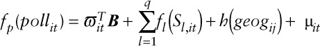
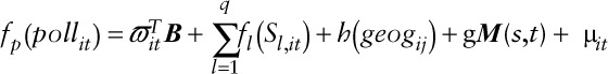
We developed spatio-temporal semiparametric models, of the form:

where is the measurement of the air pollutant at location on day , is an unspecified smooth function reflecting the nonlinear effect of covariate on the transformed pollutant concentration , stands for the smoothed covariate; is a bivariate smooth function of geographical coordinates (latitude and longitude) accounting for residual correlation between locations and ; ϖ_it is the vector of covariates that have a linear effect on ; B is the corresponding vector of regression coefficients; and 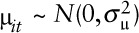. For NO₂, 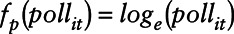and for O₃,

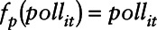
Dispersion

The Community Multiscale Air Quality (CMAQ-urban) model^16,17 combines emissions data with the Weather Research and Forecasting (WRF) meteorological model v3.6.1 (National Centre for Atmospheric Research, Boulder, CO),¹⁸ and the Community Multiscale Air Quality (CMAQ) model v5.0.2 (U.S. Environmental Protection Agency, Washington, DC),¹⁹ which has been coupled to the Atmospheric Dispersion Modeling System (ADMS) roads model v4 (Cambridge Environmental Research Consultants, Cambridge, UK).²⁰ For this study, the anthropogenic emissions data were obtained by combining the UK National Atmospheric Emissions Inventory (NAEI),²¹ the London Atmospheric Emissions Inventory,²² King’s road transport emissions model,²³ and the European Monitoring and Evaluation Programme European emissions.²⁴ The biogenic emissions from vegetation and soils were estimated using the Biogenic Emission Inventory System version 3 (BEIS3) model (U.S. Environmental Protection Agency).²⁵ Sea-salt emissions were calculated in line in CMAQ. The CMAQ-urban model outputs hourly air pollution concentrations at 20 m grid resolution across study domain. The model provides nitrogen oxides (NO_X), NO₂ and O_3, with the ADMS roads model used to describe the near field dispersion from roadways and NO₂ and O₃, using a simple chemical scheme.²⁶

Hybrid models

Hybrid1: For each pollutant, we constructed a combined LUR-dispersion model by incorporating into the LUR, daily predicted air pollutant values estimated from the CMAQ-urban dispersion model at fixed-site air pollution monitoring locations, as a nonlinear covariate. The resulting models took the form:

where is a spatio-temporal spline representing the CTM model predictions with coefficient, .

Hybrid2: For each pollutant, using R version 3.3.3 (R Foundation for Statistical Computing, Vienna, Austria),²⁷ and library mgcv with generalized cross-validation smoothing,²⁸ a generalized additive model (GAM) approach was applied to combine predicted pollutant concentrations at fixed-site monitoring locations from the developed spatio-temporal LUR and CMAQ-urban dispersion models. The GAM was developed by fitting two corresponding splines of the predicted variables to measurements at fixed monitoring sites. For the LUR, we used 10-fold cross-validated predictions.

Validation data

For dispersion modeling, validation data consisted of model NO₂ and O₃ predictions for 2009–2013 for all monitoring sites, linked to their corresponding monitor measurements, which played no role in the modeling. For models that included monitoring data in the modeling process (i.e., LUR, hybrid1, and hybrid2), a 10% leave-out rule was used by which 10% of monitors were omitted, the model recalibrated, and used to predict pollutant outputs at the left-out sites. This process was repeated until a full model-monitor dataset was achieved, predicting values for the complete set of monitors.

Simulation strategy

Following the same general approach as detailed in our previous article,⁵ our simulation strategy consisted of 4 basic steps:

Step1: Simulating “true” daily mean outdoor air pollutant data for the geographic centroid of each LSOA using a simple pollutant site-type specific spatio-temporal model developed from monitor measurements in our validation datasets. As in our previous article,⁵ the model incorporated spatio-temporal variances and covariances as well as adjusting for instrument error in the monitor measurements.

Step2: Simulating “true” outcome data from the “true” pollutant data, incorporating a relationship between the two based on a multilevel Poisson regression model,¹⁰ with three prespecified regression coefficients representing: baseline disease rate ; the short-term concentration-response function (CRF) per 1 µg/m³ change in pollutant (); and the long-term CRF per 1 µg/m³ change in pollutant (). The values of these coefficients used for each pollutant and outcome combination are listed in eTable 1; http://links.lww.com/EE/A86.

Step3: Simulating pseudo-modeled daily pollutant data from the “true” pollutant data prespecifying both the temporal () and spatial () Pearson correlation coefficients between the two and their temporal () and spatial () variance ratios (model versus “true”). For each pollution model, pollutant, and site type, these parameters were estimated from an analysis of validation data with correction for instrument error in monitor measurements as described in ePage 3; http://links.lww.com/EE/A86.

Step4: Refitting the multilevel Poisson regression model, replacing “true” pollutant data with the corresponding pseudo-modeled data. This provides us with estimates of and (i.e., expressed per 10 µg/m³) and their corresponding standard errors.

For NO₂, we considered not only additive measurement error but proportional error (i.e., additive on a log scale). Proportional error scenarios use log_e(NO₂) as the pollutant leading to the simulation of “true” log_e(NO₂) data and pseudo-modeled log_e(NO₂) data. Simulated “true” and pseudo-modeled log_e(NO₂) data are back-transformed to NO₂ for simulating “true” outcome data and refitting the Poisson regression model, respectively.

Simulations were run in R version 3.4.3,²⁷ using libraries Hmisc,²⁹ lme4,³⁰ MASS,³¹ and foreign.³²

Performance assessment

For each combination of pollutant (NO₂ [with additive or proportional error], O₃ [with additive error]), site type, pollution model, and outcome, we ran 1,000 simulations and obtained 1,000 estimates of: , from which we calculated, for both long and short-term exposure, the average health effect estimate, average standard error, percent bias in health effect estimation, coverage probability as the percentage of 95% confidence intervals containing the true concentration-response function, and power as the percentage of significance tests that were statistically significant at the 5% level.³³ Using our simulated health effect estimates, we tested for differences from their respective “true” values by calculating simple one-sample t-tests.

Standard performance metrics

For each pollutant, pollution model, and site type, we also calculated: mean bias; normalized mean bias; normalized mean gross error; root mean square error; and FAC2 (i.e., fraction of estimates within a factor of 2).^2,3

Results

Table 1 contains estimated correlation coefficients and variance ratios obtained from the validation datasets and used to define our scenarios. It illustrates that in a real-world example, the spatial and temporal variance ratios may differ quite markedly as can the spatial and temporal correlation coefficients. The hybrid1 model provided out-of-plausible range predictions for one roadside/kerbside O₃ monitoring site, resulting in a large spatial variance ratio and a small negative spatial correlation coefficient (Table 1).

Table 1.

Estimates of correlation coefficients and variance ratios^a comparing model and “true” data within sites and between sites, respectively.

Simulation results

Simulation findings for all-cause mortality are summarized in Tables 2–4. For all pollutant-site-type scenarios, the LUR exposure estimates produced a sizeable downward bias in the estimated health effect of long-term exposure ranging from −91% for roadside/kerbside NO₂ to −68% for roadside/kerbside O₃. For short-term exposure, bias also tended to be negative though not as large (i.e., −56% to −23%), although for urban/suburban O₃, bias was small and positive (4%). When dispersion exposure estimates were used, negative biases were generally smaller, substantially in some cases, and the previously positive bias for short-term exposure to urban/suburban O₃ became negative (−18%). Including dispersion outputs as an additional covariate in the LUR model produced out-of-plausible exposure range predictions for one roadside/kerbside O₃ monitoring site and only marginal improvements in health effect estimation for other pollutant site-type combinations. However, combining both LUR and dispersion predictions in a generalized additive model tended to minimize bias in health effect estimates, which ranged from −28% to 11% for long-term exposure and −17% to 11% for short-term exposure.

Table 2.

All-cause mortality and NO₂ (measurement error: additive): .

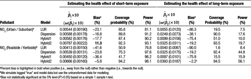
Table 4.

All-cause mortality and O₃ (measurement error: additive): .

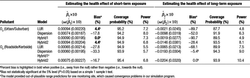
The hybrid2 model also appeared optimal for coverage probability and statistical power, with values of the former ranging from 92.3% to 95.4% and values of the latter for short-term exposure to NO₂ ranging from 84.2% to 98.1%. For long-term exposure, due to smaller sample size, and for short-term exposure to O₃, due to a very small CRF, statistical power was much lower but was nevertheless, with one exception, (short-term exposure to urban/suburban O₃) higher for the hybrid2 model than for the other modeling approaches. For the dispersion model, the lowest (worst) coverage probability was 75.3% observed for short-term exposure to roadside/kerbside NO₂ (proportional error), although the corresponding figure for long-term exposure was 92.4%. For LUR, coverage probabilities for O₃ scenarios were greater than 87%. However, this was not the case for NO₂, especially for long-term exposure at roadside/kerbside sites, where a coverage probability of 0% was obtained.

Results from our simulations based on hospital admissions for cardiovascular disease can be found in eTables 2–4; http://links.lww.com/EE/A86; and exhibit similar patterns to mortality.

Standard performance metrics

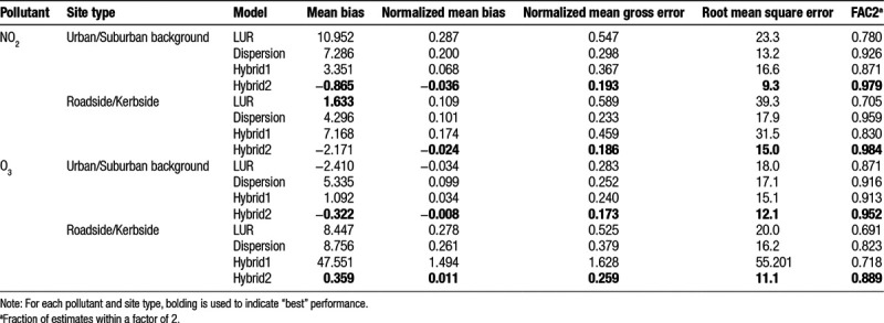
Validation statistics of mean bias, normalized mean bias, normalized gross mean error, root mean square error, and FAC2 (Table 5) also favored the hybrid2 model. Nevertheless, it is noteworthy that the LUR model produced the lowest mean bias for roadside/kerbside NO₂ (i.e., the smallest absolute difference between modeled and measured daily mean NO₂ concentrations averaged across roadside/kerbside sites).

Table 5.

Standard validation statistics calculated for each monitoring site and then averaged over sites.

Discussion

Summary of findings and context

We find that with either additive or multiplicative error, the bias induced in health studies is negative (i.e., towards the null) and generally substantially negative. From our simulation results and standard performance metrics, the hybrid2 model combining LUR and dispersion predictions was the preferred choice for use in a multilevel analyses of air pollution and health within the London area, in terms of minimizing the downward bias.

Standard measurement error theory considers two error types, that is, classical and Berkson.³⁴ Additive classical error is evidenced by a high variance ratio (model versus “true”) and generally leads to downward bias in health effect estimates, underestimation of standard errors and reduced coverage of 95% confidence intervals, whereas pure additive Berkson error is evidenced by a low variance ratio (model versus “true”) and results in inflated standard errors and reduced statistical power.^34,35 However, measurement error introduced into modeled air pollution data may be more complex. This has led Szpiro et al,¹ in the context of LUR modeling, to describe classical-like error (i.e., behaving like classical error) introduced by parameter estimation and Berkson-like error introduced by oversmoothing. Given that total measurement error depends not only on the variances of both modeled and “true” data but also on their covariance, it is important to consider not only the variance ratio (model versus “true”) but also the correlation coefficient (model versus “true”) when assessing the impact of both classical/classical-like and Berkson/Berkson-like error in an epidemiological analysis.⁵ Here and in line with the findings of our previous simulation work,⁵ we observed some small bias away from the null when a high correlation was paired with a low variance ratio and substantial bias towards the null when a high variance ratio was paired with a low correlation coefficient (Tables 1–4).

Based on our simulations, the LUR model predictions performed well for short-term exposure to urban/suburban O₃, producing only a small positive bias in the health effect estimate, although for long-term exposure bias was large and negative. For scenarios involving NO₂, the dispersion model rather than the LUR model consistently produced lower bias, higher coverage probability, and higher statistical power.

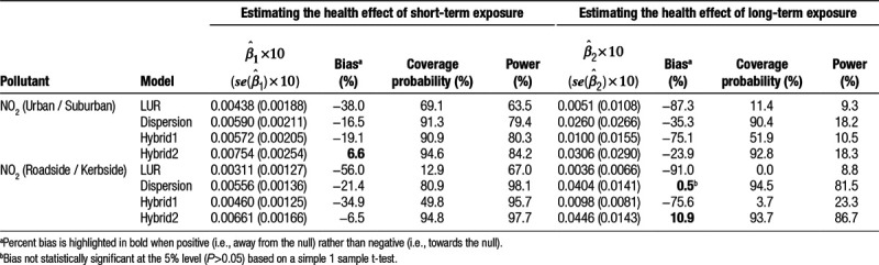
For NO₂, which is often found to have a positive skew distribution, we explored the effects of both additive and proportional measurement error, but contrary to some other simulation studies,^6,7 observed few differences in our results (see Tables 2 and 3). However, when we plotted histograms of site-mean corrected NO₂ measurements by site type, we observed little positive skew, which may explain these findings.

Table 3.

All-cause mortality and NO₂ (measurement error: proportional): .

Some writers have argued that substantial upward bias can result from measurement error in air pollution studies. For example, Crump³⁶ conducted simulation studies in linear regression and reported upward bias with proportional measurement error, whereas we generally observed downward bias in our simulations with proportional error. We think this likely reflects his focus on a restricted set of dose-response relationships (Y~bXⁿ), whereas our analysis examines the more usual case of a log-linear relationship.

Standard metrics of exposure error, such as mean bias, which address the issue of how closely the model predicts true exposure on a daily basis, provide limited insight into the magnitude of biases introduced into a complex epidemiological analysis and may, in some instances, be misleading. For example, in Table 5, for roadside/kerbside NO₂, the LUR model produced the smallest mean bias, and yet, our simulations indicate that its use in a multilevel analysis of air pollution and health, leads to substantial underestimation of health effect estimates for both short-term and long-term exposure, poor coverage probabilities, and low statistical power. Nevertheless, when various standard metrics were viewed as a whole, they supported our overall conclusion.

Possible explanations

Given our validation data compares modeled output to monitoring data and is, therefore, focused on a point (i.e., the coordinates of the monitoring station), we might expect the LUR model to have an advantage. However, the LUR is trained at monitoring sites whose distribution is not random, and this may provide a disadvantage for predictions at other locations, including held out monitoring stations. Further, the dispersion model predicts to a high level of spatial resolution (i.e., 20 m) and then estimates pollutant exposure at a point using bilinear interpolation. The high spatial resolution of the dispersion model and the use of the 10% leave-out method for the LUR model may explain part of our findings, although the fact that the dispersion model performed better overall especially with respect to the traffic-related pollutant (NO₂) may suggest that the LUR is simply missing some potentially important covariates or more complex associations between those considered. Nevertheless, as Szpiro et al¹ found in their simulation study, simply dropping an important variable from a correctly specified LUR may have little impact on health effect bias, as any loss of prediction accuracy may be counter-balanced by a reduction in the amount of classical measurement error introduced through model parameter estimation.

When a spline in the dispersion output was added to the LUR model as a covariate, the overall improvement in performance was marginal. The superiority of hybrid2, therefore, suggests that the performance of both LUR and dispersion outputs may not be uniform across the range of pollutant exposures and that combining them using penalized splines within a GAM facilitates better compensation of one for the deficiencies of the other. Di et al³⁷ has recently reported that using penalized splines to ensemble average different predictors for particulate matter of diameter <2.5 μm also reduced error precisely because the relative fit between models changed with concentration.

Study strengths and limitations

The statistical model used within our simulations enabled us to estimate the within-LSOA effect of short-term exposure and the between-LSOA effect of long-term exposure. Details of the model and a consideration of its strengths and limitations can be found in the original article by Kloog et al.¹⁰

It is possible that some bias observed in our health effect estimates is an artifact of random error introduced by the simulation procedure itself. However, this bias is likely to be small, as evidenced from our one-sample t-tests for all-cause mortality (Tables 2–4), which were significant for all bias estimates >4.4% away from the null or >5.4% towards the null.

One advantage of our study is that we tried to evaluate and correct for classical measurement error in the day to day monitored data so that the variance ratios and correlation coefficients used in our simulations better-reflected comparisons between modeled and “true” data as opposed to modeled and monitored data.^5,7,8 Having generated “true” data with given spatio-temporal variation and spatial covariance, we then simulated pseudo-modeled data from the “true” by using these metrics (i.e., the correlation coefficients and variance ratios) to introduce measurement error (see ePage 7; http://links.lww.com/EE/A86 for checks on simulations). This approach did not specifically allow for the fact that measurement error introduced by spatio-temporal modeling maybe both heteroscedastic and spatially correlated.³⁸ Nevertheless, some of the variance ratio / correlation coefficient combinations obtained from the validation study naturally introduced a lack of independence between the Berkson component and pseudo-modeled data and / or the classical component and “true” data. One limitation of our approach is that it does not provide insight into the effects of including covariates in the analysis, which, if correlated with the pollutant of interest, may lead to additional bias in health effect estimation. The nature of this bias depends on many factors, including the type of error in the pollution data (i.e., classical, Berkson, additive, proportional), whether the covariates are themselves measured with error, the relationship between the pollutant data and the covariates, and whether their respective measurement errors are correlated.³⁹ Thus, although some of these issues have been considered by other simulation studies,⁹ they are very specific to the covariates or combinations of covariates to be included and whether the same covariates have been used in developing the air pollution model e.g. temporal covariates in LUR models.

Conclusions

Although our study is confined to the London area and four examples of different modeling approaches, it illustrates how the choice of air pollution model or combination thereof can be informed by using simulation as well as more conventional validation metrics.

Conflict of interest statement

The authors declare that they have no conflicts of interest with regard to the content of this report.

ACKNOWLEDGMENTS

We are grateful to the UK Met Office for provision of meteorological data, accessed through the Centre for Environmental Data Analysis (CEDA). We are also grateful to the UK Government and Local Authorities providing air pollution measurements used in this study, managed by King’s College London and Ricardo Energy and Environment. B.K.B. analyzed the validation data, conducted the simulations, and took the lead in designing the simulations and drafting the article. E.S. contributed to the simulation design. B.B. constructed the monitoring dataset. S.D.B. and N.K. constructed the dispersion model, and K.D. constructed the LUR and hybrid models. S.D.B., N.K., and K.D. used their respective models to produce pollutant predictions at fixed monitoring sites. K.K., R.W.A., B.B., S.D.B., E.S., J.W.S., and B.K.B. were involved in the study design. All authors contributed to the drafting of the article, read and approved the final version.

References

- 1.Szpiro AA, Paciorek CJ, Sheppard L. Does more accurate exposure prediction necessarily improve health effect estimates? Epidemiology. 2011;22:680–685. [DOI] [PMC free article] [PubMed] [Google Scholar]
- 2.Thunis P, Pernigotti D, Gerboles M. Model quality objectives based on measurement uncertainty. Part I: ozone. Atmos Environ. 2013;79:861–868. [Google Scholar]
- 3.Thunis P, Pederzoli A, Pernigotti D. Performance criteria to evaluate air quality modelling applications. Atmos Environ. 2012;59:476–482. [Google Scholar]
- 4.Lin C, Heal MR, Vieno M, et al. Spatiotemporal evaluation of EMEP4UK-WRF v4.3 atmospheric chemistry transport simulations of health-related metrics for NO2, O3, PM10 and PM2.5 for 2001-2010. Geosci Model Dev. 2017;10:1767–1787. [Google Scholar]
- 5.Butland BK, Samoli E, Atkinson RW, Barratt B, Katsouyanni K. Measurement error in a multi-level analysis of air pollution and health: a simulation study. Environ Health. 2019;18:13. [DOI] [PMC free article] [PubMed] [Google Scholar]
- 6.Strickland MJ, Gass KM, Goldman GT, Mulholland JA. Effects of ambient air pollution measurement error on health effect estimates in time series studies: a simulation-based analysis. J Expo Sci Environ Epidemiol. 2015;25:160–166. [DOI] [PMC free article] [PubMed] [Google Scholar]
- 7.Goldman GT, Mulholland JA, Russell AG, et al. Impact of exposure measurement error in air pollution epidemiology: effect of error type in time-series studies. Environ Health. 2011;10:61. [DOI] [PMC free article] [PubMed] [Google Scholar]
- 8.Butland BK, Armstrong B, Atkinson RW, et al. Measurement error in time-series analysis: a simulation study comparing modelled and monitored data. BMC Med Res Methodol. 2013;13:136. [DOI] [PMC free article] [PubMed] [Google Scholar]
- 9.Dionisio KL, Chang HH, Baxter LK. A simulation study to quantify the impacts of exposure measurement error on air pollution health risk estimates in copollutant time-series models. Environ Health. 2016;15:114. [DOI] [PMC free article] [PubMed] [Google Scholar]
- 10.Kloog I, Coull BA, Zanobetti A, Koutrakis P, Schwartz JD. Acute and chronic effects of particles on hospital admissions in New-England. PLoS One. 2012;7:e34664. [DOI] [PMC free article] [PubMed] [Google Scholar]
- 11.Department of Communities and Local Government. English Indices of Deprivation - LSOA level. Available at: https://data.gov.uk/dataset/english-indices-of-deprivation-2015-lsoa-level. Accessed 25 September 2017. Licenced under the Open Government Licence (OGL) v3.0. Available at: http://www.nationalarchives.gov.uk/doc/open-government-licence/version/3/.
- 12.London Air Quality Network. King’s College, London. Available at: http://www.londonair.org.uk/. Accessed 1 March 2017.
- 13.Air Quality England. Ricardo Energy and Environment. Available at: http://www.airqualityengland.co.uk/. Accessed 1 March 2017.
- 14.Automatic Urban and Rural Network (AURN) Data Archive. © Crown 2017 copyright Defra via uk-air.defra.gov.uk, licenced under the Open Government Licence (OGL) v2.0. Available at: http://www.nationalarchives.gov.uk/doc/open-government-licence/version/2/. Accessed 1 March 2017.
- 15.Met Office (2012): Met Office Integrated Data Archive System (MIDAS) Land and Marine Surface Stations Data (1853-current). NCAS British Atmospheric Data Centre. Available at: http://catalogue.ceda.ac.uk/uuid/220a65615218d5c9cc9e4785a3234bd0. Accessed 1 May 2018. [Google Scholar]
- 16.Beevers SD, Kitwiroon N, Williams ML, Carslaw DC. One way coupling of CMAQ and a road source dispersion model for fine scale air pollution predictions. Atmos Environ. 2012;59:47–58. [DOI] [PMC free article] [PubMed] [Google Scholar]
- 17.Williams ML, Lott MC, Kitwiroon N, et al. The Lancet Countdown on health benefits from the UK Climate Change Act: a modelling study for Great Britain. Lancet Planet Health. 2018;2:e202–e213. [DOI] [PubMed] [Google Scholar]
- 18.Skamarock WC, Klemp JB, Dudhia J, et al. A Description of the Advanced Research WRF Version 3 (No. NCAR/TN–475+STR). 2008.Boulder, USA: University Corporation for Atmospheric Research. [Google Scholar]
- 19.Byun DW, Ching JKS. Science Algorithms of the EPA Models-3 Community Multiscale Air Qualty (CMAQ) Modelling System EPA/600/R-99/030 (NTIS PB2000-10561). 1999.Washington, DC: U.S. Environmental Protection Agency. [Google Scholar]
- 20.CERC. ADMS roads v4 User Guide. Available at: http://www.cerc.co.uk/environmental-software/assets/data/doc_userguides/CERC_ADMS-Roads4.1.1_User_Guide.pdf. Accessed February 2018.
- 21.Defra. Emissions of Air Quality Pollutants 1990-2014. 2016. Defra, UK. Available at: https://uk-air.defra.gov.uk/assets/documents/reports/cat07/1609130906_NAEI_AQPI_Summary_Report_1990-2014_Issue1.1.pdf. Accessed February 2018. The Data are © Crown 2019 copyright Defra & BEIS via naei.beis.gov.uk, licenced under the Open Government License version 2.0. Available at: http://www.nationalarchives.gov.uk/doc/open-government-licence/version/2/. [Google Scholar]
- 22.Greater London Authority (GLA). The London Atmospheric Emissions Inventory 2013. 2016. Available at: https://data.london.gov.uk/dataset/london-atmospheric-emissions-inventory-2013. Accessed February 2018.
- 23.Beevers SD, Westmoreland E, de Jong MC, Williams ML, Carslaw DC. Trends in NOX and NO2 emissions from road traffic in Great Britain. Atmos Environ. 2012;54:107–116. [Google Scholar]
- 24.EMEP/CEIP. Present state of emission data. 2014. Available at: https://www.ceip.at/webdab_emepdatabase/reported_emissiondata/. Accessed 21 October 2019.
- 25.Vukovich JM, Pierce TE. The Implementation of BEIS3 within the SMOKE modeling framework. Available at: https://www3.epa.gov/ttn/chief/conference/ei11/modeling/vukovich.pdf. Accessed 9 December 2019.
- 26.Carslaw DC, Beevers SD. Estimations of road vehicle primary NO2 exhaust emission fractions using monitoring data in London. Atmos Environ. 200539:167–177. [Google Scholar]
- 27.R Core Team. R: A language and environment for statistical computing. 2017. Vienna Austria: R Foundation for Statistical Computing. Available at: https://www.R-project.org/. Accessed 14 April 2020. [Google Scholar]
- 28.Wood S. mgcv: Mixed GAM computation vehicle with automatic smoothness estimation. 2017. R package version 1.8-17. Available at: https://CRAN.R-project.org/package=mgcv. Accessed 14 April 2020.
- 29.Harrell FE, Jr; with contributions from Dupont C and many others. Hmisc: Harrell miscellaneous. 2016. R package version 4.0-2. Available at: http://CRAN.R-project.org/package=Hmisc. Accessed 14 April 2020.
- 30.Bates D, Maechler M, Bolker B, Walkers S. Fitting linear mixed-effects models using lme4. J Statist Software. 2015;67:1–48. [Google Scholar]
- 31.Venables WN, Ripley BD. Modern Applied Statistics with S. 2002.4th edNew York: Springer. [Google Scholar]
- 32.R Core Team. Foreign: Read data stored by Minitab, S, SAS, SPSS, Stata, Systat, Weka, dBase … Rpackage version 0.8-63. 2015. Available at: https://CRAN.R-project.org/package=foreign. Accessed 14 April 2020.
- 33.Burton A, Altman DG, Royston P, Holder RL. The design of simulation studies in medical statistics. Stat Med. 2006;25:4279–4292. [DOI] [PubMed] [Google Scholar]
- 34.Armstrong BG. Effect of measurement error on epidemiological studies of environmental and occupational exposures. Occup Environ Med. 1998;55:651–656. [DOI] [PMC free article] [PubMed] [Google Scholar]
- 35.Sheppard L, Burnett RT, Szpiro AA, et al. Confounding and exposure measurement error in air pollution epidemiology. Air Qual Atmos Health. 2012;5:203–216. [DOI] [PMC free article] [PubMed] [Google Scholar]
- 36.Crump KS. The effect of random error in exposure measurement upon the shape of the exposure response. Dose Response. 2006;3:456–464. [DOI] [PMC free article] [PubMed] [Google Scholar]
- 37.Di Q, Amini H, Shi L, et al. An ensemble-based model of PM2.5 concentration across the contiguous United States with high spatiotemporal resolution. Environ Int. 2019;130:104909. [DOI] [PMC free article] [PubMed] [Google Scholar]
- 38.Szpiro AA, Sheppard L, Lumley T. Efficient measurement error correction with spatially misaligned data. Biostatistics. 2011;12:610–623. [DOI] [PMC free article] [PubMed] [Google Scholar]
- 39.Carroll RJ, Ruppert D, Stefanski LA, Crainiceanu CM. Measurement Error in Nonlinear Models: A Modern Perspective. 2006:2nd ed. Chapman & Hall/CRC Taylor & Frances Group, Boca Raton. 52– 63–55, 64. [Google Scholar]
Associated Data
This section collects any data citations, data availability statements, or supplementary materials included in this article.