Daily surveillance of COVID-19 using the prospective space-time scan statistic in the United States

Highlights

• •Prospective space-time statistics are particularly useful for COVID-19 surveillance.
• •Daily cluster detection can track the evolution of key hotspots of COVID-19.
• •Temporal trend towards smaller but more numerous clusters.
• •Time-periodic surveillance of COVID-19 facilitates decision-making in public health.
• •Web application for live results http://covid19scan.net.

Graphical abstract

Abstract

The severe acute respiratory syndrome coronavirus 2 (SARS-CoV-2) was first discovered in late 2019 in Wuhan City, China. The virus may cause novel coronavirus disease 2019 (COVID-19) in symptomatic individuals. Since December of 2019, there have been over 7,000,000 confirmed cases and over 400,000 confirmed deaths worldwide. In the United States (U.S.), there have been over 2,000,000 confirmed cases and over 110,000 confirmed deaths. COVID-19 case data in the United States has been updated daily at the county level since the first case was reported in January of 2020. There currently lacks a study that showcases the novelty of daily COVID-19 surveillance using space-time cluster detection techniques. In this paper, we utilize a prospective Poisson space-time scan statistic to detect daily clusters of COVID-19 at the county level in the contiguous 48 U.S. and Washington D.C. As the pandemic progresses, we generally find an increase of smaller clusters of remarkably steady relative risk. Daily tracking of significant space-time clusters can facilitate decision-making and public health resource allocation by evaluating and visualizing the size, relative risk, and locations that are identified as COVID-19 hotspots.

1. Introduction

First discovered in late 2019 in Wuhan City, China  (Huang, Wang, Li, Ren, Zhao, Hu, Zhang, Fan, Xu, Gu, et al., 2020, Li, Guan, Wu, Wang, Zhou, Tong, Ren, Leung, Lau, Wong, et al., 2020), the severe acute respiratory syndrome coronavirus 2 (SARS-CoV-2), may cause novel coronavirus disease 2019 (COVID-19) in symptomatic individuals. There have been over 7,000,000 confirmed cases and over 400,000 confirmed deaths globally since December of 2019; and in the United States (U.S.), over 2,000,000 cases were confirmed and over 110,000 confirmed deaths counted  (Dong et al., 2020). Due to the challenges of developing a vaccine for SARS-CoV-2, it will likely take another year or more until the public is sufficiently protected from COVID-19  (Lurie et al., 2020). Therefore, it is important to monitor the spread of the disease systematically, anticipate or detect new outbreaks early, analyze past and existing clusters to gain insights about spatiotemporal trends, and facilitate response efforts.

An efficient and effective public health response to disease outbreaks, including stay-at-home orders, testing, and the allocation of hospital resources, relies on the collection and timely analysis of case data, which is commonly referred to as disease surveillance  (Yang, 2017). It is an integral part of health emergency work and has contributed to saving lives during the COVID-19 pandemic by slowing and preventing transmission, optimizing care, and minimizing the impact on health care delivery systems  (WHO, 2020). Space-time scan statistics  (Kulldorff, 1997, Kulldorff, Athas, Feurer, Miller, Key, 1998, Kulldorff, Huang, Pickle, Duczmal, 2006) are a family of popular and extensively utilized techniques for disease surveillance and early detection, as they identify geographic and temporal clusters of elevated disease risk while quantifying cluster strength and statistical significance. Space-time scan statistics have been applied for analyzing chikungunya and dengue fever in Colombia and Panama  (Desjardins, Whiteman, Casas, Delmelle, 2018, Whiteman, Desjardins, Eskildsen, Loaiza, 2018), detecting West Nile Virus infection hot spots in Italy  (Mulatti et al., 2015), identifying areas of increased crime activity  (Han et al., 2019), and for rapid surveillance of COVID-19 cases in the United States  (Desjardins et al., 2020), among others.

During a pandemic, surveillance may require analyzing data streams of daily updated case counts for dynamic disease risk mapping  (Hay et al., 2013). In such a scenario, periodic (e.g. daily) application of the prospective space-time scan statistic is beneficial  (Kulldorff, 2001), as it detects active or emerging clusters of the current day, while disregarding past clusters that may have ceased to pose a public health threat  (Greene et al., 2016). It therefore allows for tracking of existing clusters while detecting new ones as the phenomenon of interest unfolds. Time-periodic surveillance using the prospective space-time scan statistic has been carried out for early detection of terrorism outbreaks  (Gao et al., 2013), thyroid cancer among men,  (Kulldorff, 2001), and syndromic surveillance in Massachusetts  (Takahashi et al., 2008), among others. Time-periodic surveillance is especially suitable to monitor the development of COVID-19 daily case counts in the United States, as lockdown measures are currently being relaxed, businesses reopen, and people start engaging in social activities again.

Effectively disseminating the results of the abovementioned disease surveillance efforts is critical and should inform both researchers and the general public to improve the understanding of the spread and risk of COVID-19. As such, the COVID-19 pandemic has resulted in a wide variety of online dashboards that display the power of geographic information coupled with information regarding the pandemic at various levels of aggregation. For example, the Johns Hopkins coronavirus dashboard is the most followed and utilized online resource for daily updates about cases, deaths, and hospitalizations, and other key information about COVID-19 in the United States and across the globe  (Dong et al., 2020). COVID Control1 is another Johns Hopkins dashboard that uses volunteered geographic information  (Goodchild, 2007) for syndromic surveillance of COVID-19 related symptoms at the county level in the U.S. Additional examples of COVID-19 dashboards include the World Health Organization, HealthMap, China’s close contact detector geosocial app, WorldPop  (Boulos and Geraghty, 2020), among a plethora of other local, regional, national, and global platforms. Since the objective of this paper is to conduct daily surveillance of COVID-19 cases, we developed our own interactive dashboard to examine the evolution of significant space-time clusters that can be viewed and utilized by both researchers and public audiences.

This study continues and improves upon previous and ongoing COVID-19 surveillance efforts that use the prospective space-time scan statistic on confirmed cases at the county level in the United States  (Amin, Hall, Church, Schlierf, Kulldorff, 2020, Desjardins, Hohl, Delmelle, 2020). To our knowledge, this study is the first to detect clusters of COVID-19 on a daily basis using the time-periodic prospective space-time scan statistic, tracks their characteristics through time, and offers a web application for live results. In addition, this article includes innovative figures and graphs that aid identifying spatiotemporal patterns of COVID-19. This approach is especially useful because it allows for daily identification and characterization of active and emerging clusters of COVID-19 to inform public health authorities, decision-makers and the general public about optimal locations and times to put in place measures to slow disease transmission (”flatten-the-curve”). We rerun our prospective analysis each day as case counts are updated for early detection of emerging clusters, monitoring of existing ones, and to locate counties where disease transmission is slowing down, and COVID-19 may no longer pose a threat to public health.

2. Data and methods

2.1. COVID-19 case counts

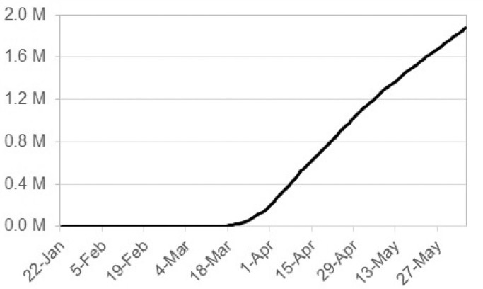
We obtained daily case counts from the COVID-19 Data Repository by the Center for Systems Science and Engineering (CSSE) at Johns Hopkins University. The repository contains case counts at the county level for the U.S., which are updated daily in tabular format. We collected daily case counts for counties within the contiguous U.S. from the day of the first confirmed case to the day of carrying out the analysis (January 22nd–June 5th, 2020). From the U.S. census website, we gathered 2018 ACS 5-year estimates of the total population at the county level and assigned them to geographic information systems (GIS) compatible county geometries. To maintain integrity of our analysis, we disregarded confirmed cases from the ”Diamond Princess” and ”Grand Princess” cruise ships, as well as cases which were designated to administrative units other than counties (states, cities, hospital districts). Because the COVID-19 case counts are cumulative for each day (Fig. 1 ), we obtained the number of new cases each day (a requirement for the space-time scan statistic) by subtracting the previous day’s count.

Fig. 1.

Cumulative number of cases between January 22nd and June 5th, 2020.

2.2. Prospective space-time scan statistic

To achieve our objective of daily COVID-19 surveillance, we utilize a Poisson prospective space-time scan statistic, which was implemented in SaTScan^TM  (Kulldorff, 2001, Kulldorff, Kulldorff, Athas, Feurer, Miller, Key, 1998). This method finds the most likely clusters from a number of cylindrical candidate clusters. The cylinders are determined by a circular base (the spatial scanning window) which is centered on a candidate location (county centroids) and that has a radius r. The height of the cylinder is determined by the temporal scanning window t. Therefore, each county centroid is the center of a number of candidate clusters of differing radii and heights. We restricted the spatial and temporal scanning windows to include 10% or less of the population at-risk and 50% or less of the study period, respectively. In addition, each candidate must contain at least 5 cases and have a minimum duration of 2 days. This parameterization is consistent with previous analyses of COVID-19 within the contiguous United States  (Desjardins, Hohl, Delmelle, 2020, Hohl, Delmelle, Desjardins, 2020).

We compute the expected and observed numbers of cases for each cylinder and perform a maximum likelihood test with null hypothesis H ₀: “There is no difference in risk of COVID-19 between the inside and outside of the cylinder”, and alternative hypothesis H_A: “There is a higher risk of COVID-19 inside the cylinder.” We compute the number of expected cases μ using Eq. (1):

$$\mu =p*\frac{C}{P}$$ (1)

with the population inside the cylinder p, the total number of cases C, and the total population P. Clusters of elevated disease risk are identified using the likelihood ratio (LR) test in Eq. (2):

$$\frac{L\left(Z\right)}{L_0}=\frac{{\left(\frac{n_Z}{\mu \left(Z\right)}\right)}^{n_Z}{\left(\frac{N-n_Z}{N-{\mu }_{\left(Z\right)}}\right)}^{N-n_Z}}{{\left(\frac{N}{\mu \left(T\right)}\right)}^N}$$ (2)

with likelihood function L(Z) for candidate cylinder Z, likelihood function L ₀ for H ₀; the number of cases inside the cylinder n_z; the expected number of cases μ(Z) in cylinder Z; the number of observed cases for the entire study area during the entire study period N; and the total number of expected cases in the study area across all time periods μ(T). Elevated risk is indicated by a likelihood ratio greater than 1, which is the case if $\frac{n_Z}{\mu \left(Z\right)}>\frac{N-n_Z}{N-{\mu }_{\left(Z\right)}}$. The cylinder with the highest likelihood ratio is the most likely cluster. The LR is a measure of how risk within a cylinder differs from risk outside, and typically its logarithmic transformation is reported as the log likelihood ratio (LLR).

We run 999 Monte Carlo simulations for significance testing, where we randomize the locations and times of the cases to obtain a likelihood ratio for each run and candidate cluster that form a distribution under H ₀. Furthermore, we include statistically significant (p < .05) secondary clusters in our reporting. Lastly, to illustrate the distribution of risk inside clusters, we report choropleth maps that contain relative risk (RR), which is the risk within a county divided by the risk outside.

Therefore, we compute Eq. (3) for each within-cluster county:

$$R{R}_{cty}=\frac{c/e}{(C-c)/(C-e)}$$ (3)

with the total number of cases c for a given county, the number of expected cases in a county e, and C the number of observed cases in the U.S. e is computed analogous to μ in Eq. (1), but using the population inside the county instead of population within a cylinder. Similarly, we compute the overall relative risk for the reported clusters (RR_{c lu}).

As opposed to its retrospective variant, the prospective space-time scan statistic finds clusters that are “active” or “emerging” at the end of the study period. While the procedure of selecting the most likely clusters from a set of candidate cylinders is the same as discussed previously, the prospective analysis only evaluates cylinders that have a “current” ending time. Therefore, the set of candidate cylinders is reduced to only include “active” cylinders at the end of the study period  (Kulldorff, 2001). In other words, only those cylinders with an end date equal to the end of the study period are considered by prospective analyses. Computation of likelihood ratio tests is the same as in retrospective scan analyses (Eq. 2).

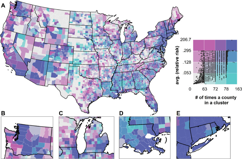
We conduct time-periodic disease surveillance, therefore we ran the prospective Poisson space-time scan statistic every day since the start of the study period (January 22nd, 2020) until the day of writing (June 5th, 2020). Each daily run of the prospective space-time scan statistic produced a most likely cluster, as well as a set of secondary clusters. Rather than examining these clusters in isolation, we are interested in how their characteristics change in space and time. Therefore we create various visuals to illustrate the dynamics of the process: (1) a series of small multiples, which tracks the change of cluster locations, their size, and their spatial relationships through time2 , (2) time series graphs that include various characteristics of the clusters for each day of the study period (Table 1 ) and (3) a bivariate map that illustrates the relationship between average relative risk across the entire study period (RR_T) and the number of days each county was part of a cluster (N_C), as observed when the prospective Poisson space-time scan statistic was computed. The latter is particularly useful to more effectively reveal relationships between two variables than a side-by-side comparison of the corresponding variables. We also (4) build a covid19scan web application where we report maps in daily increments.

Table 1.

Cluster characteristics.

Abbrev.	Characteristic
nClus	The number of clusters resulting from prospective Poisson space-time scan statistic.
nCty	Number of counties that are part of a cluster.
avgDur	Average duration of clusters.
avgRad	Average cluster radius.
cluPop	Total population within the clusters of a given day.
cluObs	Number of observed cases within clusters.
cluExp	Number of expected cases within clusters.
LLR	Log likelihood ratio.
RRclu	Cluster Relative risk.

2.3. Web application: covid19scan

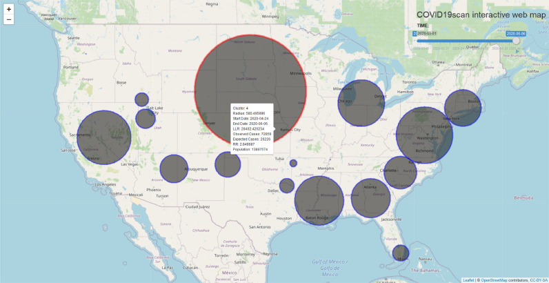
We conduct automated daily surveillance of COVID-19 for the contiguous U.S. and create a web application to report live results from the prospective space-time scan statistic3 . The application is updated daily and contains significant clusters for every day from January 22nd, 2020 to the current day overlaid on a standard OpenStreetMap4 basemap. covid19scan features standard map controls, such as zoom and pan. In addition, the map has a time slider, which allows for selecting a specific day for which clusters are displayed. The time slider also allows for animating the display of daily clusters. Lastly, the cluster characteristics mentioned previously are displayed within popup boxes that appear upon hovering over the clusters. The application is written in R  (Team, 2019) and leverages the R Shiny library  (Chang et al., 2018) for web capability and leaflet  (Cheng et al., 2018) for mobile-friendly interactive maps. We host the application using shinyapps.io5 , a service to deploy web applications through RStudio  (Team et al., 2015).

3. Results

3.1. Space-time clusters of COVID-19

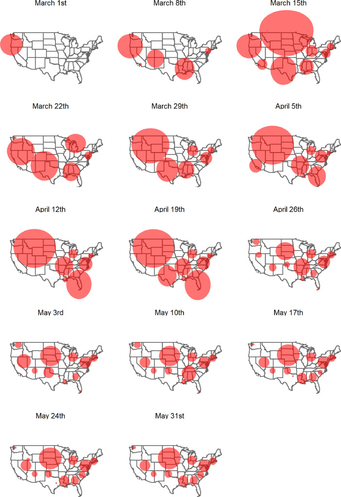
The prospective space-time Poisson scan statistic detected no significant clusters for the first 38 days of analysis. Therefore, the first cluster for the contiguous U.S. was identified in the Pacific Northwest region on March 1st, 2020 (Fig. 2 ). A week later, we observed clusters in New York, the Gulf Coast area, and the Southwestern U.S. New York and surrounding areas are part of a cluster for every day since Westchester County had an outbreak on March 5th. The following period of approximately one month is characterized by clusters of very large size, especially in the Midwest. Starting April 26th, clusters become smaller and seemingly more numerous. In the following time period, we also observe clusters that are localized to specific urban areas (Miami, FL; New Orleans, LA; Dallas, TX). Clusters are observed in each of the 5 major regions of the contiguous U.S. (West, Midwest, Northeast, Southeast, Southwest).

Fig. 2.

Weekly clusters resulting from the prospective Poisson space-time scan statistic.

Execution time of the prospective Poisson space-time scan statistic using SaTScan^TM software was 384 s for generating clusters on June 5th, 2020. Note that execution time at the beginning of the study period was shorter because of the decreased search space for the scan statistic, i.e. the number of candidate clusters to evaluate was smaller because the study period was shorter. We used a dedicated Windows 10 machine with Intel Core i3-8100 CPU at 3.6 GHz clock speed and 16 GB RAM.

3.2. Cluster characteristics

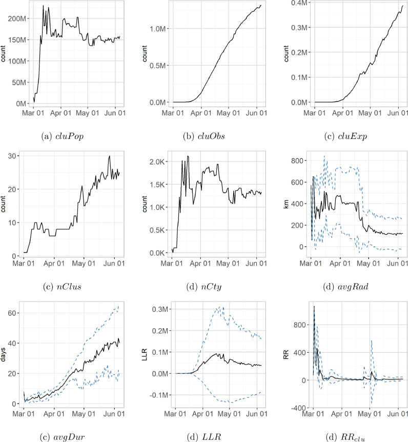
After a steep incline followed by a period of considerable variation, the total population found within the clusters produced by the prospective Poisson space-time scan statistic for a given day (cluPop) levels at around 150,000,000 (Fig. 3 a). As expected, the within-cluster number of observed cases (cluObs) exhibits a steady linear increase starting around April 19^th (Fig. 3b), with a maximum of  1,200,000 cases at the end of the study period. Similarly, the number of expected cases (cluExp) shows a linear increase, but this increase is interrupted by brief periods of decline (Fig. 3c). The periods of decline can be explained by the total cluster area, a function of the number of clusters and their radii. If the total cluster area shrinks, i.e. by a “contraction” of clusters, the within-cluster population decreases, and which causes cluExp to decrease as well (see Eq. 1).The number of clusters (nClus) varies between 6–10 clusters during the first half of the study period (after an initial increase from 0), but then increases rapidly to around 23–24 clusters towards the end of the study period (Fig. 3d). The within-cluster number of counties (nCty) exhibits a similar curve like the population: After an initial increase to around 2100, the number of counties levels in at around 1250 in the second half of the study period (Fig. 3e). The clusters vary in size and duration: Average cluster radii (avgRad) vary from 60–650 km, and we see a marked decline in size, as well as in variation of size (standard deviation), after April 26^th (Fig. 3f). Expectedly, the cluster duration (avgDur) increases during the course of the pandemic to an average duration of 39 days at the end of the study period. Interestingly, the avgDur standard deviation increases considerably during the second half of the study period to a maximum of 17 days at the end of the study period (Fig. 3g). The average log-likelihood ratio (LLR) peaks halfway through the study period at around 93,000, meaning clusters are strongest in the week of April 16th - April 23rd. This period is followed by a decline and a leveling at an LLR of 50,000 towards the end of the study period (Fig. 3h). The second half of the study period is also characterized by a peak of the LLR standard deviation, indicating clusters of substantially different strength. Lastly, average cluster relative risk (RR_{c lu}) peaks at the beginning of the study period, then sharply declines with a smaller spike in RR during the first two weeks of May.

Fig. 3.

Cluster characteristics over time. Solid black lines - summary statistic (sum or mean), dashed blue lines - standard deviation.

3.3. County-level relative risk and duration in a cluster

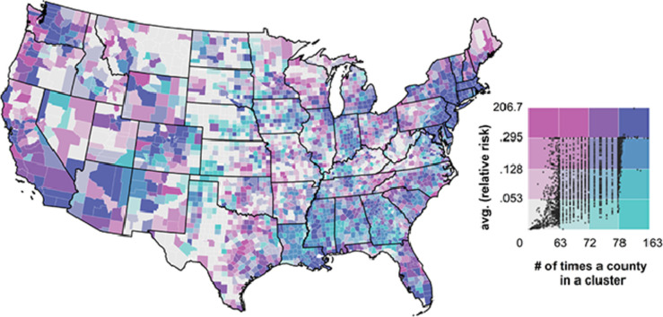
For each county, we computed the average relative risk throughout the study period (RR_T). Additionally, we recorded the number of times each county was part of a cluster (N_C), as observed when the prospective Poisson space-time scan statistic was computed. These two metrics are illustrated in a bivariate map in Fig. 4 , where variation along the green gradient corresponds to an increase of cluster membership, while variation along the pink gradient denotes a higher relative risk. The general trend is that populated counties (especially the ones encompassing and surrounding large metropolitan regions) were characterized by high average relative risk, and several times reported in clusters throughout the study period. A few illustrative examples include Seattle (inset B), Chicago and Detroit (inset C), New Orleans (inset D) and the New York City area (inset E), and also Atlanta, Miami, Salt Lake City and Denver among others.

Fig. 4.

County-level average relative risk (RR_T, natural logarithm) and duration in a cluster throughout the study period (N_C). Inset maps B,C,D, and E denote Washington state, the Chicago-Detroit area, the New Orleans region and surrounding of New York City, respectively.

Noteworthy are several counties in Louisiana, Mississippi, Alabama and Southwest Georgia which had a somewhat average relative risk yet were reported many times as clusters. Counties in Maine, western Pennsylvania (with the exception of Pittsburgh), eastern Tennessee, the western section of Virginia, West Virginia, southern Illinois, Minnesota, northern Wisconsin, Missouri, Iowa, North and South Dakota, Nebraska, Oklahoma, northern and western Texas, eastern Montana, norther Idaho, eastern Oregon, rural Nevada and Utah ranked relatively low on both metrics.

3.4. covid19scan

The covid19scan application is accessed through http://covid19scan.net and allows exploring up-to-date clusters, as well as their characteristics from an internet browser (Fig. 5 ). Temporal dynamics of clusters can be analyzed using the animation, which can be manually controlled through the time slider. Clusters of interest can be further explored by hovering over, which prompts a pop-up box that contains detailed characteristics.

Fig. 5.

The covid19scan web application.

4. Discussion

In this study, we perform time-periodic surveillance of COVID-19 in the contiguous United States using a prospective space-time scan statistic. We detect emerging clusters of COVID-19 in the United States at the county level, and provide daily results during the study period of January 22nd, 2020 - June 5th, 2020. To our knowledge, this is the first effort of conducting daily surveillance of COVID-19 utilizing the prospective space-time scan statistic to detect and characterize emerging clusters within the United States. Our work is an improvement on previous work  (Desjardins, Hohl, Delmelle, 2020, Hohl, Delmelle, Desjardins, 2020), as we apply the same methodology, but in a refined analysis using daily increments. In addition, we include informative figures that illustrate the changing cluster characteristics as the COVID-19 pandemic unfolds. Lastly, we created a web application that allows tracking the spatiotemporal distribution of significant clusters within the United States, further enhancing our existing analysis as we allow discovery of COVID-19 clusters at an increased temporal resolution (daily vs. 2–3 temporal snapshots) during a longer study period (136 days).

The time-periodic application of the prospective space-time scan statistic is attractive because of its ability to consider updated COVID-19 case counts every day while tracking existing clusters of previous days. While it identifies emerging areas of concern, it also allows for tracking the characteristics of the previously detected clusters, e.g. to determine whether they are growing or shrinking in magnitude, or whether relative risk is increasing or not. These capabilities allow for evaluating current strategies for controlling the spread of COVID-19, and offer a basis for anticipating future development of hot spots. We illustrate the benefits of the prospective approach and present a study of confirmed COVID-19 cases, which showcases the evolution of hot spots in the U.S. As a result, the number of clusters rose from 0 to 23 during our study period. At the end of our study period (June 5^th, 2020), the strongest clusters are found in the New York - Connecticut-Rhode Island region, southern Michigan and the DMV area (Washington D.C., Maryland, Virginia).

Despite the contributions of our study, there are a number of limitations and assumptions. First, we applied the prospective space-time scan statistic in its basic form, which generates clusters of circular shape. Circles may be a poor choice in a study area that exhibits substantial spatial heterogeneity. This is evident as many of the clusters we detect extend far into the oceans, which is unrealistic. Many research efforts have focused on addressing the circular dictate to allow for clusters of arbitrary shape: Elliptic scan statistics perform well if the true cluster has an elongated shape  (Kulldorff et al., 2006). Flexibly shaped scan statistics  (Tango and Takahashi, 2005) define the scanning window by connecting the k-nearest neighbors to the focus region (i.e. counties), and work particularly well for detecting clusters of irregular shape. This approach was further refined using a genetic algorithm with a penalty for geometric non-compactness  (Duczmal et al., 2007). Lastly, the spatial scan statistic was adapted to network space  (De Oliveira et al., 2011), therefore further relaxing the circular assumption. Second, like many other statistics, the prospective spatial scan statistic suffers from the multiple testing problem  (Noble, 2009), which may lead false positive clusters  (Correa et al., 2015). It is possible to correct for multiple testing, e.g. by using Bonferroni adjustment  (Shaffer, 1995), but SaTScan^TM offers a recurrence interval measurement instead, which quantifies the likelihood of observing a cluster by chance. We checked the recurrence intervals for our analyses and found that they closely follow the p-values we used for identifying clusters. The prospective space-time scan statistic has undeniable benefits for disease surveillance and is utilized by many public health authorities across the globe. Its use is recommended under consideration of the recurrence intervals available in SaTScan^TM  (Kulldorff and Kleinman, 2015). Third, the number of confirmed cases is largely a function of testing efforts and therefore, might not represent the true magnitude and spatial distribution of the virus. This concern is nourished by reports of asymptotic carriers, which might not appear in our statistics  (Bai et al., 2020). Implementing large-scale testing is the only way to address this issue. Fourth, some of the clusters we identified are very large and of limited value for disease mitigation. As a result, they may exhibit considerable variation of risk within. Performing local analyses of such areas can help identifying communities and regions in danger of COVID-19 outbreaks. Fifth, because we chose the small multiples approach for illustrating the distribution of clusters (Fig. 2), we were forced to show clusters in weekly instead of daily increments due to space limitations. Illustrating the clusters within a space-time cube framework can address this issue  (Nakaya and Yano, 2010).

5. Conclusions

Using public COVID-19 case data of the contiguous United States, provided by Johns Hopkins University’s Center for Systems Science and Engineering, we performed daily surveillance of emerging space-time clusters at the county level. We track clusters and their characteristics through space and time, and create a web application for continued COVID-19 surveillance. We find that the number of clusters is stable at the end of our study period, and that clusters decrease in size over time. In addition, within-cluster relative risk is very stable after an initial period of fluctuation at the beginning of our study period, with the exception of a spike at the beginning of May. Counties that belong to an emerging cluster can be prioritized for resource allocation and isolation measures to “flatten the curve”. The automated time-periodic use of the prospective space-time scan statistic is beneficial for monitoring COVID-19, as outbreaks can be monitored as they unfold and case counts are updated. Focusing on active clusters is important during the course of an epidemic, as previous clusters are dismissed because they may no longer pose a public health threat. Overall, geographic studies are critical for pandemic response, providing a set of methods and tools to promptly inform decision-makers about the spatiotemporal development of disease outbreaks.

Declaration of Competing Interest

None.

References

- Amin R., Hall T., Church J., Schlierf D., Kulldorff M. Geographical surveillance of covid-19: diagnosed cases and death in the united states. medRxiv. 2020 [Google Scholar]
- Bai Y., Yao L., Wei T., Tian F., Jin D.-Y., Chen L., Wang M. Presumed asymptomatic carrier transmission of covid-19. JAMA. 2020;323(14):1406–1407. doi: 10.1001/jama.2020.2565. [DOI] [PMC free article] [PubMed] [Google Scholar]
- Boulos, M. N. K., Geraghty, E. M., 2020. Geographical tracking and mapping of coronavirus disease COVID-19/severe acute respiratory syndrome coronavirus 2 (sars-cov-2) epidemic and associated events around the world: how 21st century gis technologies are supporting the global fight against outbreaks and epidemics. [DOI] [PMC free article] [PubMed]
- Chang W., Cheng J., Allaire J., Xie Y., McPherson J. Shiny: web application framework for r, 2015. R Pckage Version. 2018;1(0):14. [Google Scholar]
- Cheng J., Karambelkar B., Xie Y. Leaflet: create interactive web maps with the javascriptleafletlibrary. R Package Version. 2018;2(1) [Google Scholar]
- Correa T.R., Assunção R.M., Costa M.A. A critical look at prospective surveillance using a scan statistic. Stat. Med. 2015;34(7):1081–1093. doi: 10.1002/sim.6400. [DOI] [PubMed] [Google Scholar]
- De Oliveira D.P., Neill D.B., Garrett Jr J.H., Soibelman L. Detection of patterns in water distribution pipe breakage using spatial scan statistics for point events in a physical network. J. Comput. Civil Eng. 2011;25(1):21–30. [Google Scholar]
- Desjardins M., Hohl A., Delmelle E. Rapid surveillance of COVID-19 in the united states using a prospective space-time scan statistic: detecting and evaluating emerging clusters. Appl. Geogr. 2020:102202. doi: 10.1016/j.apgeog.2020.102202. [DOI] [PMC free article] [PubMed] [Google Scholar]
- Desjardins M., Whiteman A., Casas I., Delmelle E. Space-time clusters and co-occurrence of chikungunya and dengue fever in colombia from 2015 to 2016. Acta Trop. 2018;185:77–85. doi: 10.1016/j.actatropica.2018.04.023. [DOI] [PubMed] [Google Scholar]
- Dong E., Du H., Gardner L. An interactive web-based dashboard to track covid-19 in real time. Lancet Infect. Dis. 2020;20(5):533–534. doi: 10.1016/S1473-3099(20)30120-1. [DOI] [PMC free article] [PubMed] [Google Scholar]
- Duczmal L., Cançado A.L., Takahashi R.H., Bessegato L.F. A genetic algorithm for irregularly shaped spatial scan statistics. Computat. Stat. Data Anal. 2007;52(1):43–52. [Google Scholar]
- Gao P., Guo D., Liao K., Webb J.J., Cutter S.L. Early detection of terrorism outbreaks using prospective space–time scan statistics. Prof. Geogr. 2013;65(4):676–691. [Google Scholar]
- Goodchild M.F. Citizens as sensors: the world of volunteered geography. GeoJournal. 2007;69(4):211–221. [Google Scholar]
- Greene S.K., Peterson E.R., Kapell D., Fine A.D., Kulldorff M. Daily reportable disease spatiotemporal cluster detection, new york city, new york, usa, 2014–2015. Emerging Infect. Dis. 2016;22(10):1808. doi: 10.3201/eid2210.160097. [DOI] [PMC free article] [PubMed] [Google Scholar]
- Han M., Matheny M., Phillips J.M. Proceedings of the 27th ACM SIGSPATIAL International Conference on Advances in Geographic Information Systems. 2019. The kernel spatial scan statistic; pp. 349–358. [Google Scholar]
- Hay S.I., George D.B., Moyes C.L., Brownstein J.S. Big data opportunities for global infectious disease surveillance. PLoS Med. 2013;10(4) doi: 10.1371/journal.pmed.1001413. [DOI] [PMC free article] [PubMed] [Google Scholar]
- Hohl A., Delmelle E., Desjardins M. Rapid detection of covid-19 clusters in the united states using a prospective space-time scan statistic: an update. SIGSPATIAL Special. 2020;12(1):2733. doi: 10.1145/3404111.3404116. [DOI] [Google Scholar]
- Huang C., Wang Y., Li X., Ren L., Zhao J., Hu Y., Zhang L., Fan G., Xu J., Gu X. Clinical features of patients infected with 2019 novel coronavirus in wuhan, china. Lancet. 2020;395(10223):497–506. doi: 10.1016/S0140-6736(20)30183-5. [DOI] [PMC free article] [PubMed] [Google Scholar]
- Kulldorff M. A spatial scan statistic. Commun. Stat.-Theory Methods. 1997;26(6):1481–1496. [Google Scholar]
- Kulldorff M. Prospective time periodic geographical disease surveillance using a scan statistic. J. R. Stat. Soc.) 2001;164(1):61–72. [Google Scholar]
- Kulldorff, M., 2018. SatscanTM user guide for version 9.6, 2018.
- Kulldorff M., Athas W.F., Feurer E.J., Miller B.A., Key C.R. Evaluating cluster alarms: a space-time scan statistic and brain cancer in los alamos, new mexico. Am. J. Public Health. 1998;88(9):1377–1380. doi: 10.2105/ajph.88.9.1377. [DOI] [PMC free article] [PubMed] [Google Scholar]
- Kulldorff M., Huang L., Pickle L., Duczmal L. An elliptic spatial scan statistic. Stat. Med. 2006;25(22):3929–3943. doi: 10.1002/sim.2490. [DOI] [PubMed] [Google Scholar]
- Kulldorff M., Kleinman K. Comments on a critical look at prospective surveillance using a scan statisticby t. correa, m. costa, and r. assunção. Stat. Med. 2015;34(7):1094. doi: 10.1002/sim.6430. [DOI] [PMC free article] [PubMed] [Google Scholar]
- Li Q., Guan X., Wu P., Wang X., Zhou L., Tong Y., Ren R., Leung K.S., Lau E.H., Wong J.Y. Early transmission dynamics in wuhan, china, of novel coronavirus–infected pneumonia. N top N. Engl. J. Med. 2020 doi: 10.1056/NEJMoa2001316. [DOI] [PMC free article] [PubMed] [Google Scholar]
- Lurie N., Saville M., Hatchett R., Halton J. Developing covid-19 vaccines at pandemic speed. N top N. Engl. J. Med. 2020;382(21):1969–1973. doi: 10.1056/NEJMp2005630. [DOI] [PubMed] [Google Scholar]
- Mulatti P., Mazzucato M., Montarsi F., Ciocchetta S., Capelli G., Bonfanti L., Marangon S. Retrospective space–time analysis methods to support west nile virus surveillance activities. Epidemiol. Infect. 2015;143(1):202–213. doi: 10.1017/S0950268814000442. [DOI] [PMC free article] [PubMed] [Google Scholar]
- Nakaya T., Yano K. Visualising crime clusters in a space-time cube: an exploratory data-analysis approach using space-time kernel density estimation and scan statistics. Trans. GIS. 2010;14(3):223–239. [Google Scholar]
- Noble W.S. How does multiple testing correction work? Nat. Biotechnol. 2009;27(12):1135–1137. doi: 10.1038/nbt1209-1135. [DOI] [PMC free article] [PubMed] [Google Scholar]
- Shaffer J.P. Multiple hypothesis testing. Annu Rev Psychol. 1995;46(1):561–584. [Google Scholar]
- Takahashi K., Kulldorff M., Tango T., Yih K. A flexibly shaped space-time scan statistic for disease outbreak detection and monitoring. Int J Health Geogr. 2008;7(1):14. doi: 10.1186/1476-072X-7-14. [DOI] [PMC free article] [PubMed] [Google Scholar]
- Tango T., Takahashi K. A flexibly shaped spatial scan statistic for detecting clusters. Int J Health Geogr. 2005;4(1):11. doi: 10.1186/1476-072X-4-11. [DOI] [PMC free article] [PubMed] [Google Scholar]
- Team R. Rstudio: integrated development for r. RStudio, Inc., Boston, MA URL http://www. rstudio. com. 2015;42:14. [Google Scholar]
- Team R.C. R: a language and environment for statistical computing. dim (ca533) 2019;1(1358):34. [Google Scholar]
- Whiteman A., Desjardins M., Eskildsen G., Loaiza J. Detecting space-time clusters of dengue fever in panama after adjusting for vector surveillance data. PLoS Negl Trop Dis. 2018;13(9):e0007266. doi: 10.1371/journal.pntd.0007266. [DOI] [PMC free article] [PubMed] [Google Scholar]
- WHO . Technical Report. World Health Organization; 2020. Critical Preparedness, Readiness and Response Actions for COVID-19: Interim Guidance, 22 March 2020. [Google Scholar]
- Yang W. Academic Press; 2017. Early Warning for Infectious Disease Outbreak: theory and practice. [Google Scholar]