Y-Net: Hybrid deep learning image reconstruction for photoacoustic tomography in vivo

Abstract

Conventional reconstruction algorithms (e.g., delay-and-sum) used in photoacoustic imaging (PAI) provide a fast solution while many artifacts remain, especially for limited-view with ill-posed problem. In this paper, we propose a new convolutional neural network (CNN) framework Y-Net: a CNN architecture to reconstruct the initial PA pressure distribution by optimizing both raw data and beamformed images once. The network combines two encoders with one decoder path, which optimally utilizes more information from raw data and beamformed image. We compared our result with some ablation studies, and the results of the test set show better performance compared with conventional reconstruction algorithms and other deep learning method (U-Net). Both in-vitro and in-vivo experiments are used to validated our method, which still performs better than other existing methods. The proposed Y-Net architecture also has high potential in medical image reconstruction for other imaging modalities beyond PAI.

1. Introduction

Photoacoustic tomography (PAT) is a kind of hybrid imaging modalities that combines both optical and ultrasonic imaging advantages. In PAT, ultrasonic wave is excited by a pulsed laser, which has embodied both optical absorption contrast and ultrasonic deep penetration [[1], [2], [3], [4], [5]]. Many practical applications have been investigated to show its great potential in both preclinical and clinical imaging, such as small animal whole body imaging and breast cancer diagnostics [[6], [7], [8], [9], [10], [11], [12], [13], [14], [15]]. Additionally, multispectral PAT has unique advantages in monitoring the functional information of biological tissues, such as blood oxygen saturation (sO₂) and metabolism. Specifically, photoacoustic computed tomography (PACT) enables real-time imaging performance, which reveals enormous potential for clinical applications. To obtain the image from the PA signals, image reconstruction algorithm plays an important role. Conventional non-iterative reconstruction algorithms, e.g., filtered back-projection (FBP), delay-and-sum (DAS), are prevalent due to their fast speed. However, the imperfection of conventional algorithms exists some artifacts, which results in distorted images, especially in limited view configuration. In this case, the iterative approaches are well adapted with applicable regularization.

In recent years, deep learning has been rapidly developed in computer vision area, and has begun to attract intensive research interest in image reconstruction problems for medical imaging [[16], [17], [18]]. The most non-iterative schemes are convolutional neural network (CNN) to directly reconstruct from raw data or post-process the low-quality results from conventional reconstruction [[19], [20], [21], [22], [23], [24]], which has shown satisfactory results. For example, Reiter. et al. used pre-beamformed PA data to identify point source by CNN [25]; Anas et al. proposed a new architecture that takes a low quality PA image as input restrains the noise from low power LED-based PA imaging system [26,27]; Allman et al. employed PA raw data to classify the point target from artifacts [28]; Antholzer et al. using a three-layers CNN to post process the reconstructed PA image [29]. Generally, deep learning based non-iterative methods can be divided into two categories: direct processing and post-processing. The difference between them is the format of input data: the former method feeds the raw data and converts into the image at the output of the network; the latter method feeds a poor quality image and converts the feature of the image into the final image. In addition, some learned iterative schemes train a regularization to optimize the inverse problem [[30], [31], [32]], instead of solving an optimization problem, some literatures take a well-known optimization method as basis, but by learning parts of the methods, they deviate from this method. The resulting end-to-end process mimics an optimization procedure, while they do not optimize a function containing an explicit learned regularization [[33], [34], [35]]. However, they still have to compute forward and adjoint model alternatingly. The number of iterations is restricted by GPUs with limited resources in the training phase.

The direct processing takes raw PA data as input, which only perform well in some simple target (e.g. point, line) [22,28]; the latter method takes an artifacts-distorted PA image as input, and this scheme converts reconstruction to an image processing problem [21,29]. However, both existing schemes have their disadvantages: direct processing method is difficult to map the inverse model for a complicated target (e.g. vessel) even though raw data contains more physical information of target. Besides, post-processing method has a poor generalization performance due to limited information in input and various artifacts (caused by system setup or reconstruction algorithm). To utilize the merits of both methods to enhanced performance, in this paper, we propose one possible solution combining these two schemes, a CNN-based architecture, named Y-Net, to solve the initial PA pressure reconstruction problem for PACT. It simultaneously has two inputs (measured raw PA signals and rough solution by conventional algorithm) and one output. This approach fills the gap between existing direct-processing and post-processing methods, which can be called hybrid processing method: both the measured raw data and a beamformed (BF) image are used as inputs. These two inputs contain different types of information respectively: rich details and overall textures. It has some difference from multi-model network: (1). We cannot divide it into two independent sub-networks and keep them working on this task. (2). Y-Net did not have two respective decoders (two independent U-Net models respectively fed by both reconstructed image and raw data as input), but has only a shared decoder. Moreover, it has less parameters so that Y-Net exhibits a faster running time compared with two-models network. In this work, the measured PA signals are acquired by linear array probe, which suffers limited-view problem.

The overview of this paper is arranged as follows. Firstly, we review the physical model of PAT and inverse problem. Then, we generalize the deep learning method to reconstruct the PA image. In Method section, we show a detailed description of the architecture and implementation of our proposed method. In the experiment section, we illustrate the generation of training data and the experimental setup. In Results section, we show the simulation, in-vitro and in-vivo results compared with conventional reconstruction algorithms and other deep-learning based methods, such as U-Net. Finally, we discuss some details and conclude this work followed by future work. The preliminary results were presented in EMBC 2019 [36].

2. Background

2.1. Photoacoustic imaging

PA wave is excited by a short pulse laser, and we can derive the forward solution based on Green’s function. From the PA generation equation, the propagating PA signal in both time and spatial domain p(r, t) triggered by the initial pressure p₀(r) satisfies [4]:

$$\left({\nabla }^2-\frac{1}{v_s^2}\frac{{\partial }^2}{\partial t^2}\right)p(\text{r},t)=-p_0(\text{r})\frac{d\delta (t)}{dt},$$ (1)

where v_s is the speed of sound. We can write the forward solution of PA pressure detected by transducer at position r₀ [37]:

$$p_d({\text{r}}_0,t)=\frac{\partial }{\partial t}\left[\frac{t}{4\pi }\underset{\left|{\text{r}}_0-\text{r}\right|=ct}{\iint }{p}_0(\text{r})d\Omega \right],$$ (2)

where dΩ is the solid angle of the transducer with respect to the point at r₀. For the PAT inverse problem, the main idea is to reconstruct the initial pressure p₀(r) from the raw PA signals received by transducer p_d(r₀, t).

The conventional back-projection calculates the inverse equation, which can be expressed as [38]:

$$p_0(\text{r})=\frac{1}{{\Omega }_0}{\int }_{S_0}\left[2p({\mathbf{r}}_0,t)-\frac{2t\partial p({\mathbf{r}}_0,t)}{\partial t}\right]\frac{\cos {\theta }_0}{{\left|\mathbf{r}-{\mathbf{r}}_0\right|}^2}d{S}_0,$$ (3)

where θ₀ is the angle between the vector pointing to the reconstruction point r and transducer surface.

Let f = p₀(r) and the measured data by sensor equal to b, and we use a linear operator A represent the forward model, then we have:

$$Af=b.$$ (4)

To solve the inverse problem, the main idea is recovering f from the known b.

2.2. PA image reconstruction

PA image can be reconstructed from the intact raw data by solving Eq. (1). Many pre-clinical applications require real-time imaging performance, which put computation efficiency as a basic requirement for the algorithm design. By proper approximation of these wave equations, many beamforming algorithms such as time-domain delay-and-sum and time reversal (TR) [[39], [40], [41], [42]], have been widely applied in real application due to their fast speed and easy implementation.

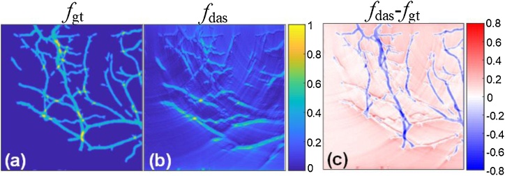
DAS is considered as one of the most commonly used beamforming algorithms in PA imaging, which has a fast reconstruction compared with other algorithms. However, it can only reconstruct a poor image with high levels of sidelobe. Fig. 1(c) indicates the difference between the images reconstructed by conventional reconstruction and ground-truth, and all PA signals are measured by a linear array transducer at the top of the region of interest. It also shows that the DAS reconstructed image loses some information depicting backbones due to severe artifacts and limited-view transducer. Fig. 1(c) is the differential image of Fig. 1(a) and (b) highlighting the major different vessels, most of which cannot receive the PA signal at the vertical orientation of the linear ultrasound array.

Fig. 1.

Comparison of information loss in the traditional DAS reconstruction method. (a) The ground-truth; (b) The delay-and-sum reconstructed result of (a); (c) The difference between (a) and (b).

Model-based approach can reconstruct the imperfect data well compared with above non-iterative algorithms, which devotes to rebuild PA image f from signal b by optimizing the objective function:

$$\underset{f}{\arg \min }\frac{1}{2}{||Af-b||}_2^2+\lambda ℛ(f),$$ (5)

where $\frac{1}{2}{||Af-b||}_2^2$ indicates the data consistency, and the R(f) is the regularizing term, λ is a regularization parameter. It can be solved in many methods iteratively [31,[43], [44], [45], [46], [47], [48]], which are time-consuming due to forward operation calculation in every iteration.

2.3. Deep learning for reconstruction

Deep-learning-based approach has been developed to resolve the image reconstruction problem. Non-iterative deep-learning-based approaches can be divided into direct and post-processing schemes. The former scheme maps the sensor data b to initial pressure f using a CNN framework, which can be generally expressed as:

$$\underset{\Theta }{\arg \min }{E}_{b,f}{||\mathcal{N}(\Theta ,b)-f||}_2^2.$$ (6)

This problem is approximately solved over a training dataset ${\left\{\left(b_i,f_i\right)\right\}}_{i=1}^N$. However, this method does not contain physical models, and is only driven by data, leading to lower generalization and robustness. On the other hand, the latter scheme considers the approximate solution of physical model and the parameters of network subject to learning are:

$$\underset{\Theta }{\arg \min }{E}_{f^{\ast },f}{||\mathcal{N}(\Theta ,f^{*})-f||}_2^2,$$ (7)

where f * is the approximate solution generated by conventional non-iterative algorithm, such as DAS. This scheme has rough texture information of the object and shows better performance compared with the previous scheme. However, the detailed information of object may be lost as the input DAS-generated images are imperfect and suffers severe artifacts.

Both abovementioned non-iterative schemes have their own drawback respectively, and current research work mostly focused on boosting the neural network. In this paper, we fill the gap between existing two approaches, and propose a new representational framework, which fuses and complements each other of the two schemes.

3. Methods

Most CNN architecture only establishes a single input-output stream for imaging reconstruction (e.g. signals only or image only). Based on above analysis, the scheme with signals’ input only or with images’ input only suffers their own drawbacks, respectively. Therefore, we assume that it may be a good solution to combine the raw PA signals and beamformed images as input data. It deserves noting that the raw PA signals and beamformed image have different size and features, which inspired us to build the neural network with two inputs.

Our proposed scheme can be termed as hybrid processing, and a pair of inputs are fed into the network to learn the parameters subject to:

$$\underset{\Theta }{\arg \min }{E}_{(f^{\ast },b),f}{||\mathcal{N}(\Theta ,b,f^{*})-f||}_2^2.$$ (8)

This scheme incorporates more texture information compared with the direct-processing scheme, and more physical information compared with the post-processing scheme. Since these schemes do not rely on complex models (only simple system model in DAS), the proposed method has the ability to satisfy real-time imaging requirements.

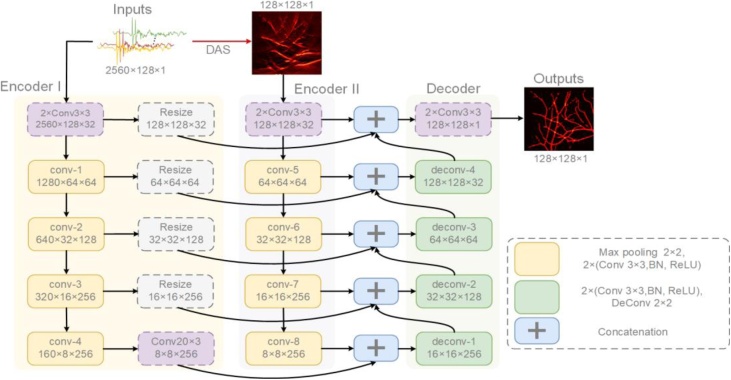
The proposed Y-Net integrates both features with two inputs by two different encoders. The global architecture of Y-Net is shown in Fig. 2, which inputs the raw PA signals to an encoder, and processes the raw data to obtain an imperfect beamformed image as the input of another encoder. Being different from U-Net [49], the proposed Y-Net enables two inputs for different types of training data that is optimized for hybrid image reconstruction. The Y-Net consists of two contracting paths and a symmetric expanding path. Encoder I and Encoder II encode the physical features and texture features respectively, and the final decoder concatenates the features of both encoder’s outputs and generates the final result.

Fig. 2.

The architecture of Y-Net. Two encoders extract different input feature, which concatenates into the decoder. Both encoders have skip connections with the decoder. DAS: delay-and-sum; (H × W×C) in blocks specify the output dimension of each component; ConvH × W indicates the convolution operations with H × W kernel size; 2× means two same layers. All operations accompanied by a Batch-Normalization(BN) and a ReLU.

3.1. Encoder for measured data

The Encoder for measured data (Encoder I) takes the raw PA signals as input. It is similar to the contracting path of U-Net. An extra 20 × 3 convolution is put on the middle of the bottom layer, which translates the 160 × 8 features map to 8 × 8. Every layer also shared their information with the Decoder mirrored layers by resizing and skipping connection. The raw data contains a complicated feature, and Encoder I filtrates the feature as a supplement for the information loss of reconstructed image during the beamforming process.

The Encoder I maps a given PA signal $b\in {ℝ}^{N_b}$ to a features space $z\in {ℝ}^{N_k}$. Assuming it only has one convolution every layer of the encoder, we can denote the i-th channel of k-th layer for Encoder I:

$${\phi }_i^k={\sigma }_2\left(P^{k\text{T}}{\sigma }_1\left({\sum }_{j=1}^{s-1}\left({\phi }_j^{k-1}\ast {\kappa }_{i,j}^k\right)\right)\right),i<s.$$ (9)

where s is the output channels size, κ is the convolutional kernel, and σ (⋅) is the batch normalization (BN) and rectified linear unit (ReLU) operation, P is pooling operation, * denotes the convolution operation. Furthermore, we also rewrite the matrix representation of the k-th layer for double convolution operation:

$${\phi }^k={\sigma }_3\left({\sigma }_2\left({\sigma }_1\left({\text{P}}^{k\text{T}}({\phi }^{k-1})\right)\ast {\kappa }_1^{k\text{T}}\right)\ast {\kappa }_2^{k\text{T}}\right),$$ (10)

all the operations are matrix operations. For the first layer, the input is measured data, without the pooling operation. We can rewrite the parameterization of Encoder I:

$$z_1=\left({\phi }^5\cdots {\phi }^1(b)\right)\ast {\kappa }_3^{5T}=E_1(w_{E1},b)\ast {\kappa }_3^{5T},$$ (11)

where w_E1 is parameter matrices: $W_{E1}\in {ℝ}^{N_5}\times \cdots \times {ℝ}^{N_1}$. The kernel ${\kappa }_3^5$ with 20 × 3 size map the feature from 160 × 8 to 8 × 8. We do not explicitly tune the bias term since it can be incorporated into φ. Meanwhile, the signals have a longer size in time-dimension, and a larger receptive field is desirable to focus more information in this dimension. Although z₁ is latent features of PA image, most dimensions are asymmetric before last convolution operation. These parameters should be estimated during the training phase.

3.2. Encoder for reconstructed image

The Encoder for reconstructed image (Encoder II) takes the image reconstructed from raw PA data by a conventional algorithm (DAS in this paper). The structure of every layer is the same as Encoder I except the bottom layer. Every layer unit is composed of two 3 × 3 convolutions, BN and ReLU, and a maximizing pooling to downsample the features. The image is passed through a series of layers that gradually downsample, and every layer acquires different information respectively. Meanwhile, every layer shared their information with the decoder mirrored layers by skip connection. It is desirable to concatenate many low-level information such that the location of texture will be passed to the decoder.

Similarly, the Encoder II maps a reconstructed PA image $f^{*}\in {ℂ}^{N*}$ to a features space $z\in {ℝ}^{M_k}$. The matrix representation of the k-th layer for Encoder II is similar to Encoder I:

$${\phi }^k={\sigma }_3\left({\sigma }_2\left({\sigma }_1\left({\text{P}}^{k\text{T}}({\phi }^{k-1})\right)\ast {\kappa }_1^{k\text{T}}\right)\ast {\kappa }_2^{k\text{T}}\right).$$ (12)

For the first layer, the input is reconstructed image without the pooling operation. We can also rewrite the parameterization of Encoder II as:

$$z_2={\phi }^5\cdots {\phi }^1(f^{*})=E_2(w_{E2},f^{*}),$$ (13)

where W_E2 is parameter matrices: $w_{E2}\in {ℝ}^{M_5}\times \cdots \times {ℝ}^{M_1}$. The reconstructed image will be encoded as latent features through the E₂.

3.3. Decoder of Y-Net

The outputs of the two encoders are taken to the decoder after concatenation, which is symmetric with Encoder II. Every layer unit is composed of two 3 × 3 convolutions, and an up-convolution to upsample the features. On the other hand, every layer receives low-level information from two encoders’ mirrored layers and concatenate with the feature from previous layer of the decoder. The final layer will generate a 128 × 128 image.

The decoder takes two feature maps from different encoder as inputs, process it and produce an output $f\in {ℂ}^N$. For the decoder, every layer is fed by two skipped connections from two encoders except the feature from the prior layer. The corresponding operation at the k-th layer encoder is described by:

$${\chi }^k={\phi }^k={\sigma }_3\left({\sigma }_2\left({\sigma }_1\left({\text{P}}^{k\text{T}}({\phi }^{k-1})\right)\ast {\kappa }_1^{k\text{T}}\right)\ast {\kappa }_2^{k\text{T}}\right),$$ (14)

where χ^k denotes the skipped feature. Particularly, the skipped feature of Encoder I needs to resize to the same dimension with other feature. Similarly, the Decoder maps these features to a final PA image $f\in {ℂ}^N$. We also rewrite the matrix representation of the k-th layer with skipped connection:

$${\phi }^k={\sigma }_3\left({\text{U}}^{k\text{T}}\left({\sigma }_2\left({\sigma }_1\left({\phi }^{k-1}\text{+R}({\chi }_1^k)+{\chi }_2^k\right)\ast {\kappa }_1^{k\text{T}}\right)\ast {\kappa }_2^{k\text{T}}\right)\right),$$ (15)

where U(⋅) is up-convolution operation, R(⋅) is the resizing operation (we compare convolution operation in Ref. [22] with resizing in Table S2 of supplementary materials). It is noteworthy that every channel of Decoder layer has triple channels including two encoder features and prior feature. For the final layer, the output is the final image, without the up-sampling operation. Meanwhile, we can rewrite the parameterization of Decoder as:

$$f={\phi }^5\cdots {\phi }^1(z_1,z_2)=D(w_D,z_1,z_2),$$ (16)

where W_D is parameter matrices: $w_D\in {ℂ}^{N_5}\times \cdots \times {ℝ}^{N_1}$. Two inputs (z₁ and z₂) are different dimensional features, which are mapped to the final image by D(⋅).

3.4. Implementation

As shown in Fig. 2, every module of convolutions contains BN and ReLU (f (x)= max (0, x)). Encoders and decoder have five layers respectively, and the output size of every layer has been annotated in the block in Fig. 2.

We use the mean squared error (MSE) loss function to evaluate the reconstructed error. Adam optimization algorithm [50] is used to optimize the network iteratively. The MSE loss is defined as:

$$L_{rec}(f)=\frac{1}{2}{||f-gt||}_F^2,$$ (17)

where f is the reconstruction image, gt is the ground-truth, and ||·||_F denotes the Frobenius norm. In our method, Encoder II encodes a reconstructed image to semantic features from image, which can be deeply supervised by image, so we should further penalize Encoder II by an auxiliary loss:

$$L_{aux}(z_2)=\frac{1}{2}{||z_2\ast {\kappa }^{\text{T}}-R(gt)||}_F^2,$$ (18)

where R(⋅) is resizing operation¹, the channels of z₂ convert to one channel by convolution with a 3 × 3 kernel κ. It can improve the learning ability of the intermediate layer, regulating hidden layer to learn discriminative features. Furthermore, fast convergence and regularization are also achieved [51,52]. We verify the auxiliary loss using an ablation study in supplementary materials. Besides, we use a large kernel with 20 size to extend the receptive field of Encoder I. Finally, we train the network by minimizing the total loss:

$$L_{total}=L_{rec}+\lambda L_{aux},$$ (19)

where λ is hyper-parameter, and we chose λ = 0.5 in the training phase.

Pytorch [53] is used to implement the proposed Y-Net. The hardware platform we used is a high-speed graphics computing workstation consisting of two Intel Xeon E5−2690 (2.6 GHz) CPUs and four NVIDIA GTX 1080Ti graphics cards. The batch size is set as 64, and the running time is 0.453 s per batch. The iteration is set as 1000 epochs, and the initial learning rate is 0.005. The source code is available at https://github.com/chenyilan/Y-Net.

4. Experiments

4.1. Numerical vessels data generation

The deep-learning-based approach is a data-driven method that requires a number of data for training to get the desired results. Unfortunately, PAT does not have access to a large amount of clinical data to train the network as a kind of newly developed imaging technology. Especially for reconstruction problems, we often need raw data, which is usually only available in research lab. Therefore, following the standard data preparation approach in deep-learning PA imaging community [20,21,33,35], we seek to train neural networks using simulation data and test the trained models in experiments both in-vitro and in-vivo.

The MATLAB toolbox k-Wave [54] is used to generate the training data. The simulation setup is shown in Fig. 3, where a linear array transducer was placed at the top of the region of interest (ROI). The sample is placed in the 38.4 × 38.4 mm size of ROI, where the linear array probe with 128 elements can receive the PA signals from the sample. The center frequency of the transducer is set as 7 MHz with 80 % fractional bandwidth. We record the raw data from the sensor, generate beamformed images and ground-truth for training and testing. All images have 128 × 128 pixels, and acoustic speed is set as 1500 m/s. The time length of every channel is set as 2560 with 33.3 MHz sampling rate. We finally allot a 2560 × 128 input size for PA sensor data, which has 60 dB SNR with added Gaussian noise. The generation speed of data is 70.79 s per image.

Fig. 3.

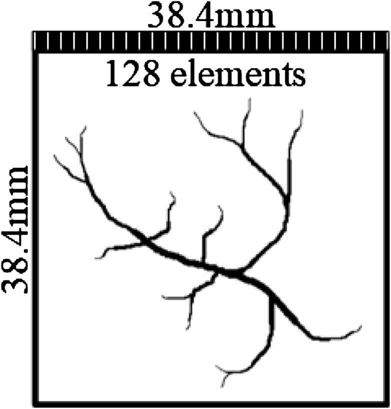
The illustration of the simulation setup.

The hemoglobin is the main strong contrast in biological soft tissue, therefore, we assume the target is vessel. The public fundus oculi vessel DRIVE [55] is used to deploy with initial pressure distribution. Considering the DRIVE data is small, the data need to be segmented and pre-processed to expand the data volume: 1). the complete blood vessel of fundus oculi is factitiously segmented into four equal parts; 2). randomly rotational transform (90°, 180°, 270°) and superpose two segmented blood vessels. After a series of operations, the excessive dataset will be loaded into k-Wave simulation toolbox as the initial pressure distribution. The dataset consists of 4700 training sets and 400 test sets.

4.2. Verification of simulation data

We trained all models on the numerical training data, and verify on the test set. In this phase, we compare our method with ablation study and some existing models as following:

• •Two variant Y-Net are used as ablation study. Y-Net-EIID removes the connection between raw data (Encoder I) and Decoder, and Y-Net-EID removes the connection between the beamformed image (Encoder II) with the Decoder.
• •The post-processing method: U-Net [49], the input is the result of DAS image.

We compare our method with the non-iterative learned method in our paper. All learned methods use the same data set and test on other data.

4.3. Application to in-vitro data

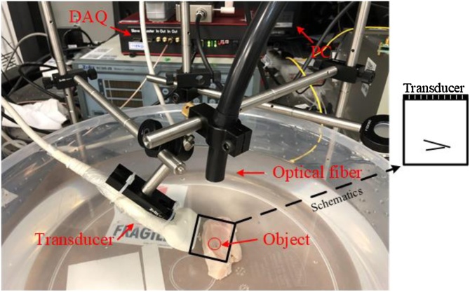
In order to further verify the feasibility of our proposed method, an in vitro phantom was prepared by a chicken breast tissue inserted with two pencil leads. The PACT system is depicted in Fig. 4: a pulsed laser (532 nm, 450 mJ, 10 Hz) illuminates the sample through an optical fiber, and a data acquisition card (DAQ-128, PhotoSound) received and amplified the PA signals from the 128 channels’ ultrasound probe (7 MHz, Doppler Inc.). In our experiment, the laser energy density is set as 9.87 mJ/cm², which is under the ANSI standards safety limit (20 mJ/cm² for 532 nm wavelength). The data sampling rate is 40 MHz (It is different from simulation, and we compare these two sampling rates in the supplementary materials), and data length is 2560 points. The system is synchronously controlled by a computer, including laser firing and data acquisition. Two leads are inserted in the chicken breast tissue as “V” shape in the black box of Fig. 4, and the ROI is the same as the simulation setup.

Fig. 4.

The schematic of PACT system setup; red circle indicates the pencil lead. DAQ: data acquisition card; PC: personal computer; black box indicates the region of interest and the schematic illustrates the position relationship between the phantoms and the ultrasonic transducer.

4.4. Application to human in-vivo data

Last but not least, the in-vivo PA imaging experiments of a human palm have also been performed to validate our approach. The system setup is the same as the in-vitro experiment. Both in-vitro and in-vivo data have different characteristics that are not perfectly represented by the training on synthetic data. The practical data suffers some noise and other environmental factors that makes the results inferior to numerical simulation experiment. The Y-Net can still perform well compared with other algorithms since the Encoder II can provide a texture to guide the reconstruction.

5. Results

5.1. Evaluation of synthetic data

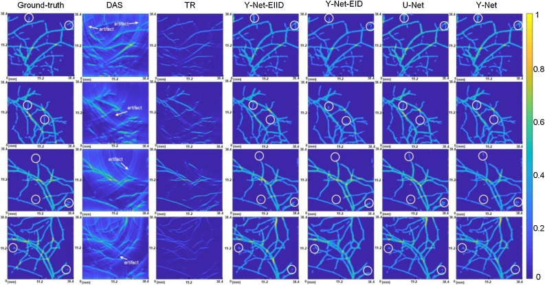
We compared two different conventional algorithms and three different models with our proposed approach. TR and DAS are selected as conventional algorithms for evaluating performance. To visually compare the performance of different methods, four examples of imaging results from the test set are shown in Fig. 5. From left to right, the method is DAS, TR, Y-Net-EIID, Y-Net-EID, post-processing U-Net and the proposed complete Y-Net. In Fig. 5, the images of TR are much dimmer than other images even though they have the same range. The reason causing the dimmer image may be that the results of TR reconstruction has sparse high value, and most of pixels are low value even though it is a valid object.

Fig. 5.

The example of performance comparison using different methods to reconstruct initial pressure. The four examples correspond to four rows; every column corresponds to different method, from left to right: ground-truth, DAS, TR, Y-Net-EIID, Y-Net-EID, post-processing U-Net and Y-Net. DAS: delay-and-sum; TR: time reversal. The white circles indicate the local details.

The conventional algorithms are easily fooled by artifacts, and we can still see the appearance of the object roughly. For the DAS results, the arrows showed that some artifacts may disturb the estimation of vessel direction due to limited-view. The deep-leaning-based approach almost restores the rough outline of the sample, and its performance differs for reconstructing the details of small vessels. On the other hand, from the local details of Fig.5 (white circles), we can see that all models with the concatenation between Encoder II and Decoder (Y-Net-EIID, Y-Net, U-Net) are susceptible to strong artifacts of input and introduced some errors in the details, and some artifacts could be retained in a few cases. The high-dimensions feature can be processed by encoder-decoder network and the texture features can be retained by skipped connections, so U-Net perform better for many segmentation tasks. Y-Net-EID can avoid the abovementioned errors, but it is difficult to identify the small independent source (No concatenation between Encoder II and Decoder may cause missing texture of beamformed image.). The proposed complete Y-Net provides a clearer texture in detail than the U-Net, which indicates that Y-Net is more anti-disturbing to artifacts in BF by integrating the information in raw data. So the performance of Y-Net may be further improved by utilizing more advanced BF algorithm.

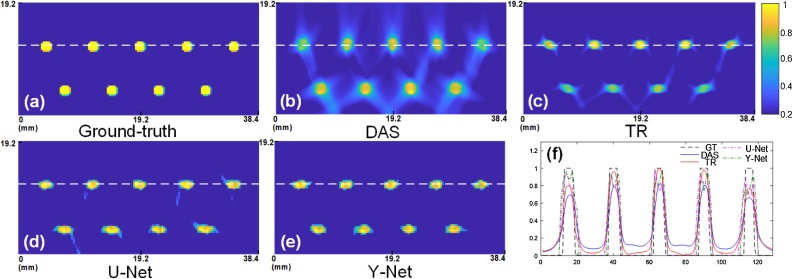
Furthermore, we can analyze the resolution using the point-target, which will help on evaluating these methods from another perspective. Nine points phantom with 1.5 mm diameter has been placed in two rows as the Fig. 6 (a) showed. We compare our method with DAS, TR and U-Net in Fig. 6 (b)-(e). In conventional algorithms, many artifacts adjoin the target points in Fig. 6 (b) and (c). In practice, most non-iterative algorithms are unable to eliminate artifacts especially in limited-view configuration. Our method eliminates most artifacts compared with U-Net, but deep-learning-based method can introduce a slight distortion due to the gap between training data and point-like data. Since Ref. [28] focused on the target on point-like source and removed their artifacts for all training and test data. It is a reasonable excuse that numerous differences between training data and point-like data caused a worse result compared with Ref. [28]. Taking a look at a horizontal cross section of the white dotted line, the profile along the white dotted line also indicates the superiority of our method compared with others in Fig.6 (f). In Fig. 6, all of images have 128 × 64 pixels’ size, but conventional results look smoother. The reason is that the conventional algorithm is physical-based methods. The results have gradual change since these methods back propagate and superimpose the PA signal on time domain. The ground-truth has a steep edge, so the results of deep learning may look like discontinuity. We can also compare the different profiles from Fig. 6 (f).

Fig. 6.

The reconstruction results of point-like phantom: (a) ground-truth; (b) delay-and-sum; (c) time reversal; (d) U-Net; (e) proposed Y-Net; (f) The profile along the white dotted line of (a), (b), (c), (d), (e).

We computed the axial resolution for the results of Fig. 6 based on the rules in [56], and list the axial resolution values measured from different reconstructions in Table 1. The theoretical resolution is calculated 0.88c/Δf, which is based on the transducer’s central frequency and bandwidth parameters. Since the lateral resolution is related to the distance between the scanning center and imaging point, and the transducer’s aperture, we compare the full width at half maximum (FWHM) value at lateral direction of middle point in Fig. 6 (f). From Table 2, we see that TR has best lateral resolution at middle position, and the Y-Net has second best resolution compared with other methods. It is worth noting that the pixel size can affect the practical resolution if the size is not sufficiently small. If the pixel size is larger than the theoretical resolution, the imaging result may not distinguish the target size that is smaller than one pixel. Therefore, the pixel size of Fig. 6 (128 × 64) also impacted the resolution in practice.

Table 1.

The axial resolution values in Fig. 6.

Algorithms	Theory	DAS	TR	U-Net	Y-Net
Resolution(μm)	148.8	907.2	756.0	453.6	332.6

Table 2.

The FWHM value at lateral direction of middle point in Fig. 6.

Algorithms	DAS	TR	U-Net	Y-Net
FWHM(μm)	2418.88	1814.16	2176.99	2146.76

Three indexes for quantitative evaluation are used as the metric to evaluate the performance of different methods:

(1). Structural Similarity Index (SSIM) [57], a higher value indicates a better quality for estimated image, which is simply defined as:

$$\text{SSIM}(f,gt)=\frac{(2{\mu }_f{\mu }_{gt}+C_1)(2{\sigma }_{\mathrm{cov}}+C_2)}{({\mu }_f^2+{\mu }_{gt}^2+C_1)({\sigma }_f^2+{\sigma }_{gt}^2+C_2)},$$ (20)

where μ_f, μ_gt and σ_f, σ_gt are the local means, and standard deviations of f and gt respectively, and σ_cov is cross-covariance for f, gt. The default values of some parameters are: C₁ equals to 0.01, C₂ equals to 0.03, dynamic range is 1, and the standard deviation of Gaussian function is 1.5 with 11 × 11 window size.

(2). The Peak Signal-to-Noise Ratio (PSNR) is a conventional metric of the image quality in decibels (dB):

$$\text{PSNR}(f,gt)=10{\log }_{10}(\frac{I_{\max }^2}{MSE}),$$ (21)

where I_max is the max value of f, gt (in this work, I_max = 1), MSE can be calculated by Eq. (17).

(3). The Signal-to-Noise Ratio (SNR) is defined as:

$$SNR(f,gt)=10{\log }_{10}\left(\frac{mean(g{t}^2)}{mean[{(gt-f)}^2]}\right),$$ (22)

where mean(·) is the mean operation. We also compare two variant Y-Net with our approach: Y-Net-EIID and Y-Net-EID. Meanwhile, the post-processing method based U-Net that only input an image after beamforming is also demonstrated for evaluation.

We can compute the quantitative evaluation of the test sets is shown in Table 3. The data volume of test set is 400, which are generated by MATLAB and described in Experiments section. Firstly, the deep learning based methods show more advantageous than conventional algorithms. Within the deep learning based approaches, the proposed network's performance is superior in comparison with the other networks. We can also compute the quantitative evaluation of Fig. 6 to compare the performance, which is shown in Table 4. The DAS shows a much worse quantitative result from Table 4 (e.g. SSIM: 0.1131 vs. 0.9079) due to the severs artifacts in Fig. 6 (b). The Y-Net performs better quantitative result compared with U-Net in Table 4 (e.g. SSIM: 0.7847 vs. 0.9079), even though look very similar in Fig. 6.

Table 3.

Quantitative evaluation of different methods for test sets (mean ± std).

Algorithms	SSIM	PSNR	SNR
DAS	0.2032 ± 0.0226	17.3626 ± 0.6775	1.7493 ± 0.8105
TR	0.5587 ± 0.0644	17.8482 ± 1.2947	2.2350 ± 0.8607
Y-Net-EIID	0.8988 ± 0.0200	25.2708 ± 1.5412	9.6577 ± 1.2035
Y-Net-EID	0.8622 ± 0.0295	23.9152 ± 1.9491	8.105 ± 1.7466
U-Net	0.9002 ± 0.0192	25.0032 ± 1.7616	9.3233 ± 1.5559
proposed Y-Net	0.9119 ± 0.0162	25.5434 ± 1.3913	9.9291 ± 1.1436

Table 4.

Quantitative evaluation of different methods in Fig. 6.

Algorithms	SSIM	PSNR	SNR
DAS	0.1131	14.8083	−0.6559
TR	0.4659	20.8807	5.4165
U-Net	0.7847	19.8829	4.5587
proposed Y-Net	0.9079	21.6401	6.1758

5.2. Evaluation of experimental data

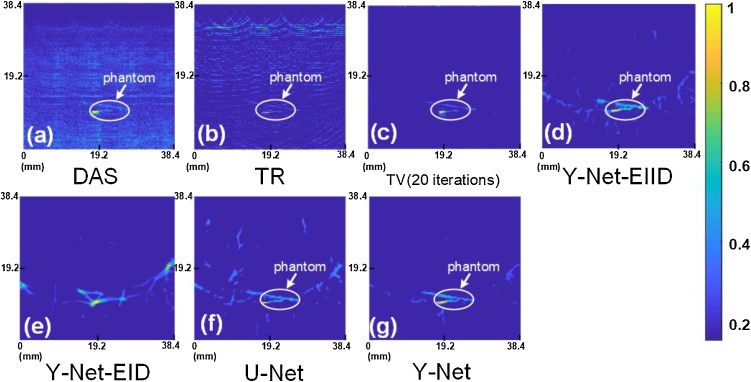
The in-vitro results are shown in Fig. 7, which also compared DAS, TR, and two variant Y-Net and U-Net with Y-Net. Considering that real experimental data has no ground-truth, we add total variation (TV) with 20 iterations as a baseline in Fig.7 (c). DAS and TR methods show poor quality due to the laser power limit and severe artifacts (Fig. 7(a)-(b)) compared with iterative method (Fig. 7 (c)), even though we still can distinguish the phantoms in the tissue. TV result shows an improved SNR and contrast in Fig. 7 (c), which clearly shows the structure of phantom after 20 iterations. Deep learning based methods also show higher SNR in Fig. 7(e)-(g). It shows that the Y-Net-EID (Fig. 7 (e)) reconstructed an incorrect image, which completely lost the shape of phantom. The skipped connection between Encoder II and Decoder is the main reason, which provides a texture feature of the sample. The phantom’s texture is different from vessel, and it causes the network to think of all signals as vessel-shape if lacking effective texture in Encoder II. U-Net removes most artifacts and retains some artifacts in extension direction, which embodies the associative ability. Y-Net shows a better result that can clearly distinguish the object (Fig. 7(g)). Fig.7 (g) retains some noises compared with Fig.7 (c), but provides a higher contrast than TV. We circled the phantom in Fig.7 and further compare the purity of background for these methods. The backgrounds of DAS and TR have more physical artifacts, which can be recognized. The backgrounds of deep learning methods are more confusing, which are erroneously identified as target except for the Y-Net.

Fig. 7.

The in-vitro result of chicken breast phantom: (a) delay-and-sum; (b) time reversal; (c) TV with 20 iterations; (d) Y-Net-EIID; (e) Y-Net-EID; (f) U-Net; (g) Y-Net.

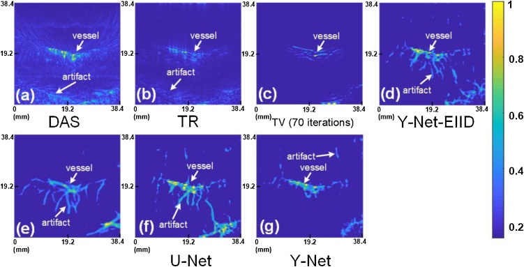
The in-vivo imaging results comparison is shown in Fig. 8, where the ROI is limited by spot size. TV with 70 iterations is also used as a baseline in Fig. 8(c). DAS and TR methods reconstructed images show many artifacts in tissue (Fig.8 (a)-(b)) compared with Fig. 8(c), but the major vessel can be recognized. Deep learning based methods have unsatisfactory results on the shape of the blood vessels due to an excessive association, especially in Fig.8 (e). We also can annotate the vessel and artifacts in Fig.8. The artifacts of DAS and TR show distinct characteristics due to underlying physics, which is easy to recognize. Deep learning methods can easy remove these physical artifacts but may create some imaginary artifacts, which may be caused by some random noise similar with vascular. Moreover, we can still obtain a denoised image using Y-Net in Fig.8 (g). These models can eliminate most noise and artifacts and still perform better than conventional methods even though they may cause some imaginary artifacts. The bottom right corner may be a vessel in deeper tissue or an intense artifact (cannot be removed after 70 iterations) from Fig. 8 (c). U-Net removes normal artifacts and connects two vessels based on the extend tendency of the vessel, which is caused by excessive association (Fig. 8(f)). However, Y-Net still showed good performance, with no excessive associations on the main blood vessel (Fig.8 (g)) and only few imaginary artifacts.

Fig. 8.

The in-vivo result of human palm: (a) delay-and-sum; (b) time reversal; (c) TV with 70 iterations; (d) Y-Net-EIID; (e) Y-Net-EID; (f) U-Net; (g) Y-Net.

The computation time for deep learning methods has been listed in Table 5, which sufficiently satisfies the requirement of real-time imaging for most applications. In Table 5, all the computation time of deep learning based methods is less than 0.04 s (equivalently more than 25 Hz). For the setup in this paper, the frame rate of imaging can achieve 12 Hz (total cost 0.08 s from raw data to final image), but limited to 10 Hz due to the repetition frequency of pulsed laser, which still satisfies the real-time imaging requirement very well.

Table 5.

The computation times for deep learning methods.

Algorithms	Time (Second)
Y-Net-EIID	0.0309
Y-Net-EID	0.0299
U-Net	0.0189
proposed Y-Net	0.0326

6. Discussions

The artifacts are essential to limited-view photoacoustic tomography. An effective strategy to reduce artifacts is a challenge in image reconstruction. For raw PA data, it is often limited by the bandwidth of transducer, which caused a loss of partial spectrum information; the linear array transducer further loses some information since it cannot capture the PA signals from all the directions, especially in vertical direction for a vessel-like sample. The model-based methods incorporate the physical model into the reconstruction process with a regularization, such as total variation (TV), and it also shows powerful performance. For imperfect conventional reconstruction algorithm (DAS), it has a fast running time through simple delaying channel data and adding them together. However, some information cannot be embodied as Fig. 1 shows. Many literatures, such as [[39], [40], [41], [42]] extracted more useful information from raw data by further improving that procedure. Besides, the non-iterative methods with Deep Learning are promising for applications where low latency is more important than a better quality reconstruction, such as real-time imaging for cancer screening and guided surgery.

Whilst DAS produced more artifacts than TR, and time-efficient approaches commonly suffer from severe artifacts. In this work, we only need a rough PA image as one of the network inputs. So the speed of the algorithm is a more important index, thus DAS is a good choice in our work compared with TR. And then, the DAS algorithm is widely used to fast reconstruct the image in US/PA imaging, and many existing US/PA systems have built-in DAS algorithm. So using DAS to generate the rough PA image can possess good compatibility with most imaging systems. In this work, we proposed a deep learning method to reconstruct PA image from raw PA signals, which can eliminate the artifacts caused by not only limited-view issue. In training stage, we applied 7 MHz with 80 % bandwidth to generate the raw data, which is close to the parameter values of the system in lab. The proposed method can easily remove these artifacts caused by both limited-view and limited-bandwidth issues. Specifically, the bandwidth can be adapted if we train the model using the same bandwidth. One flaw of using linear probe is limited-view caused artifacts as the Fig. 6(a)-(b) showed, and we used simple points as the target and they look like complete, but we can still find many artifacts around the target. However, for many complex cases such as Fig. 5, the results of vessel have some misleading artifacts caused by limited-view issue that produce severs image distortion. Therefore, our method may also process the much more severe limited-view induced artifacts issue (e.g. reflective artifacts). Some residual artifacts in Fig. 5 come from the input of Encoder II, which may be caused by the skipped connection of Encoder II. Deep learning based methods removed most artifacts but retain a part of strong artifacts. For most cases, this skipped connection can improve the performance (Y-Net > Y-Net-EIID > Y-Net-EID) and maintain texture features to avoid the pooling operation caused information loss. The ablation study also showed the superiority of skipped connection (Y-Net-EID vs. Y-Net) for most cases. For residual artifacts, we will further improve Y-Net in the future work.

In the experiments, we used the linear array probe based photoacoustic imaging setup to verify our method as the Fig. 3 showed, which is one of the mainstream system setups. The linear array has the flexibility for clinical application. Furthermore, this system setup is easy to coordinate the ultrasonic system in clinic.

The deep learning models are trained on the synthetic data since we lack many practical data for emerging photoacoustic imaging technique, which induces a gap between synthetic data and practical data. The real fabricated transducer cannot be simulated exactly alike in the simulation environment, which may cause some differences between practical signals and simulated signals. Moreover, the inestimable interferences from surroundings may distort the received data of transducer. It caused the poorer results for the in-vitro and in-vivo experiments than synthetic data. It might improve the results by altering the input of Encoder II, which can be revised as a better texture reconstructed result instead of DAS, such as [33,[37], [38], [39]]. Likewise, the results of post-processing method (U-Net) can be also improved. For the post-processing methods, the input is the preferable image, which however may lose some information as the DAS results of Fig. 5. The network repairs the information from training data, and it may cause some imaginary artifacts if only using one input as the Fig.8 (f) showed. Considering ground-truth cannot be obtained in in-vitro and in-vivo experiments, we further add an iterative result (TV with 20 iterations) in Fig. 7, Fig. 8 to help us analyze different texture. From ablation study, we see that Encoder II concatenated with Decoder can provide a main texture of output, and we will obtain an improved texture if the Encoder II is fed with a preferable input image. The Encoder I will supplement the missing information in beforehand reconstruction, and reduce the imaginary artifacts.

It is noteworthy that we premised all vessels are evenly illuminated and the medium is homogeneous in synthetic data. We cannot exclude the inhomogeneity effect of light illumination quality in the experiment, which may cause the artifacts in the results. It may be affected for all reconstruction, on the basis of which we compare the performance between these different methods, which is still reasonable. In the future work, we will further try to resolve the effect of laser illumination inhomogeneity.

In the comparative experiment, we chose U-Net as post-processing reconstruction scheme, which has been proven to work well on medical image reconstruction. In the experiment, the reconstruction results are deviated due to the gap between simulation data and measurement data, but our method still shows better performance compared to other methods.

7. Conclusions

In this paper, a new CNN architecture, named Y-Net, is proposed, which consists of two intersecting encoder paths. The Y-Net takes two types of inputs that represent the texture structure of the conventional algorithms and the high-dimensional features contained in the original raw signals respectively. Training on large dataset, Y-Net learns to distinguish the target and artifacts from raw data and polluted image. Moreover, a priori knowledge introduced from large amounts of data can compensate for information loss of vertical direction in the raw PA data. We use the k-Wave PA simulation tool to generate a large amount of training data to train the network, and evaluate our approach on the test set. In the experiment, we demonstrate the feasibility and robustness of our proposed method by comparing with other models and conventional methods. We also validated our method in in-vitro and in-vivo experiments, showing superior performance compared with existing methods. Y-Net is still affected by the artifacts of beamforming, which may be improved by using a better beamforming algorithm. In the future work, we will improve the residual artifacts and further generalize Y-Net to three dimensions for real-time 3D PA imaging.

Declaration of Competing Interest

The authors declare no conflicts of interest.

Biographies

Hengrong Lan received his bachelor degree in Electrical Engineering from Fujian Agriculture and Forestry University in 2017. Now, he is a PhD student at School of Information Science and Technology in ShanghaiTech University. His research interests are the biomedical and clinical image reconstruction, machine learning in photoacoustic and photoacoustic tomography systems design.

Daohuai Jiang received his B.S in Electrical Engineering and Automation from Fujian Agriculture and Forestry University in 2017. He is now a PhD candidate at School of Information Science and Technology in ShanghaiTech University. His research interest is photoacoustic imaging system design and its biomedical applications.

Changchun Yang received his bachelor’s degree in computer science from Huazhong University of Science and Technology in 2018. And he is pursuing his master’s degree in ShanghaiTech University. His research interest is medical image analysis and machine learning.

Feng Gao received his bachelor's degree at Xi'an University of Posts and Telecommunications in 2009 and his master's degree at XIDIAN University in 2012. From 2012–2017, he worked as a Digital Hardware Development Engineer in ZTE Microelectronics Research Institute. From 2017–2019, he worked as IC Development Engineer in Hisilicon Inc., Shenzhen. During this period, he completed project delivery of multiple media subsystems as IP development director. Various kinds of SOC chips which he participated in R&D have entered into mass production, and the corresponding products have been sold well in market. During the working period, five patents were applied. In October 2019, he joined in the Hybrid Imaging System Laboratory, ShanghaiTech University (www.hislab.cn). His research interests are image processing and digital circuit design.

Fei Gao received his bachelor degree in Microelectronics from Xi’an Jiaotong University in 2009, and PhD degree in Electrical and Electronic Engineering from Nanyang Technological University, Singapore in 2015. He worked as postdoctoral researcher in Nanyang Technological University and Stanford University in 2015−2016. He joined School of Information Science and Technology, ShanghaiTech University as an assistant professor in Jan. 2017, and established Hybrid Imaging System Laboratory (www.hislab.cn). During his PhD study, he has received Integrated circuits scholarship from Singapore government, and Chinese Government Award for Outstanding Self-financed Students Abroad (2014). His PhD thesis was selected as Springer Thesis Award 2016. He has published about 50 journal papers on top journals, such as Photoacoustics, IEEE TBME, IEEE TMI, IEEE JSTQE, IEEE TCASII, IEEE TBioCAS, IEEE Sens. J., IEEE Photon. J., IEEE Sens. Lett., ACS Sens., APL Photon., Sci. Rep., Adv. Func. Mat., Nano Energy, Small, Nanoscale, APL, JAP, OL, OE, JBiop, Med. Phys.. He also has more than 60 top conference papers published in MICCAI, ISBI, ISCAS, BioCAS, EMBC, IUS etc. He has one paper selected as oral presentation in MICCAI2019 (53 out of 1700 submissions). In 2017, he was awarded the Shanghai Eastern Scholar Professorship. In 2018 and 2019, he received excellent research award from ShanghaiTech University. His interdisciplinary research topics include hybrid imaging physics, biomedical and clinical applications, as well as biomedical circuits, systems and algorithm design.

Appendix A. Supplementary data

The following is Supplementary data to this article:

References

- 1.Wang L.V., Yao J. A practical guide to photoacoustic tomography in the life sciences. Nat. Methods. 2016;13(8):627–638. doi: 10.1038/nmeth.3925. [DOI] [PMC free article] [PubMed] [Google Scholar]
- 2.Zhou Y., Yao J., Wang L.V. Tutorial on photoacoustic tomography. J. Biomed. Opt. 2016;21(6):61007. doi: 10.1117/1.JBO.21.6.061007. [DOI] [PMC free article] [PubMed] [Google Scholar]
- 3.Zhong H., Duan T., Lan H., Zhou M., Gao F. Review of low-cost photoacoustic sensing and imaging based on laser diode and light-emitting diode. Sensors Basel (Basel) 2018;18(7) doi: 10.3390/s18072264. [DOI] [PMC free article] [PubMed] [Google Scholar]
- 4.Wang L.V. Tutorial on photoacoustic microscopy and computed tomography. Ieee J. Sel. Top. Quantum Electron. 2008;14(1):171–179. [Google Scholar]
- 5.Wang L.V., Hu S. Photoacoustic tomography: in vivo imaging from organelles to organs. Science. 2012;335(6075):1458–1462. doi: 10.1126/science.1216210. [DOI] [PMC free article] [PubMed] [Google Scholar]
- 6.Lan H., Duan T., Zhong H., Zhou M., Gao F. Photoacoustic classification of tumor model morphology based on support vector machine: a simulation and phantom study. Ieee J. Sel. Top. Quantum Electron. 2019;25(1):1–9. [Google Scholar]
- 7.Gao F., Peng Q., Feng X., Gao B., Zheng Y. Single-wavelength blood oxygen saturation sensing with combined optical absorption and scattering. IEEE Sens. J. 2016;16(7):1943–1948. [Google Scholar]
- 8.Camou S., Haga T., Tajima T., Tamechika E. Detection of aqueous glucose based on a cavity size- and optical-wavelength-independent continuous-wave photoacoustic technique. Anal. Chem. 2012;84(11):4718–4724. doi: 10.1021/ac203331w. [DOI] [PubMed] [Google Scholar]
- 9.Pleitez M.A., Lieblein T., Bauer A., Hertzberg O., von Lilienfeld-Toal H., Mantele W. In vivo noninvasive monitoring of glucose concentration in human epidermis by mid-infrared pulsed photoacoustic spectroscopy. Anal. Chem. 2013;85(2):1013–1020. doi: 10.1021/ac302841f. [DOI] [PubMed] [Google Scholar]
- 10.Lan H., Duan T., Jiang D., Zhong H., Zhou M., Gao F. Dual-contrast nonlinear photoacoustic sensing and imaging based on single high-repetition-rate pulsed laser. IEEE Sens. J. 2019 1-1. [Google Scholar]
- 11.Duan T., Lan H., Zhong H., Zhou M., Zhang R., Gao F. Hybrid multi-wavelength nonlinear photoacoustic sensing and imaging. Opt. Lett. 2018;43(22):5611–5614. doi: 10.1364/OL.43.005611. [DOI] [PubMed] [Google Scholar]
- 12.Lin L., Hu P., Shi J., Appleton C.M., Maslov K., Li L., Zhang R., Wang L.V. Single-breath-hold photoacoustic computed tomography of the breast. Nat. Commun. 2018;9(1):2352. doi: 10.1038/s41467-018-04576-z. [DOI] [PMC free article] [PubMed] [Google Scholar]
- 13.Ye F., Yang S., Xing D. Three-dimensional photoacoustic imaging system in line confocal mode for breast cancer detection. Appl. Phys. Lett. 2010;97(21) [Google Scholar]
- 14.Gao F., Feng X., Zhang R., Liu S., Ding R., Kishor R., Zheng Y. Single laser pulse generates dual photoacoustic signals for differential contrast photoacoustic imaging. Sci. Rep. 2017;7(1):626. doi: 10.1038/s41598-017-00725-4. [DOI] [PMC free article] [PubMed] [Google Scholar]
- 15.Zhang H.F., Maslov K., Sivaramakrishnan M., Stoica G., Wang L.V. Imaging of hemoglobin oxygen saturation variations in single vesselsin vivousing photoacoustic microscopy. Appl. Phys. Lett. 2007;90(5) [Google Scholar]
- 16.Wang G., Ye J.C., Mueller K., Fessler J.A. Image reconstruction is a new frontier of machine learning. IEEE Trans. Med. Imaging. 2018;37(6):1289–1296. doi: 10.1109/TMI.2018.2833635. [DOI] [PubMed] [Google Scholar]
- 17.Strack R. AI transforms image reconstruction. Nat. Methods. 2018;15(5) 309-309. [Google Scholar]
- 18.Zhang H., Dong B. A review on deep learning in medical image reconstruction. arXiv preprint arXiv. 2019;1906:10643. [Google Scholar]
- 19.Jin K.H., McCann M.T., Froustey E., Unser M. Deep convolutional neural network for inverse problems in imaging. IEEE Trans. Image Process. 2017 doi: 10.1109/TIP.2017.2713099. [DOI] [PubMed] [Google Scholar]
- 20.Cai C., Deng K., Ma C., Luo J. End-to-end deep neural network for optical inversion in quantitative photoacoustic imaging. Opt. Lett. 2018;43(12):2752–2755. doi: 10.1364/OL.43.002752. [DOI] [PubMed] [Google Scholar]
- 21.Schwab J., Antholzer S., Nuster R., Haltmeier M. DALnet: High-resolution photoacoustic projection imaging using deep learning. arXiv preprint arXiv. 2018;1801:06693. [Google Scholar]
- 22.Waibel D., Gröhl J., Isensee F., Kirchner T., Maier-Hein K., Maier-Hein L. Reconstruction of initial pressure from limited view photoacoustic images using deep learning, Photons Plus Ultrasound: imaging and sensing 2018. Int. Soc. Optics and Photonics. 2018:104942S. [Google Scholar]
- 23.Hammernik K., Würfl T., Pock T., Maier A. Springer; 2017. A Deep Learning Architecture for Limited-angle Computed Tomography Reconstruction, Bildverarbeitung Für Die Medizin 2017; pp. 92–97. [Google Scholar]
- 24.Kofler A., Haltmeier M., Kolbitsch C., Kachelrieß M., Dewey M. A U-nets cascade for sparse view computed tomography. International Workshop on Machine Learning for Medical Image Reconstruction; Springer; 2018. pp. 91–99. [Google Scholar]
- 25.Reiter A., Bell M.A.L. A machine learning approach to identifying point source locations in photoacoustic data, Photons Plus Ultrasound: imaging and sensing 2017. Int. Soc. Opt. Photonics. 2017:100643J. [Google Scholar]
- 26.Anas E.M.A., Zhang H.K., Kang J., Boctor E. Enabling fast and high quality LED photoacoustic imaging: a recurrent neural networks based approach. Biomed. Opt. Express. 2018;9(8) doi: 10.1364/BOE.9.003852. [DOI] [PMC free article] [PubMed] [Google Scholar]
- 27.E.M.A. Anas, H.K. Zhang, J. Kang, E.M. Boctor, Towards a Fast and Safe LED-Based Photoacoustic Imaging Using Deep Convolutional Neural Network, Medical Image Computing and Computer Assisted Intervention – MICCAI 20182018, pp. 159-167.
- 28.Allman D., Reiter A., Bell M.A.L. Photoacoustic source detection and reflection artifact removal enabled by deep learning. IEEE Trans. Med. Imaging. 2018 doi: 10.1109/TMI.2018.2829662. 1-1. [DOI] [PMC free article] [PubMed] [Google Scholar]
- 29.Antholzer S., Haltmeier M., Nuster R., Schwab J. Photoacoustic image reconstruction via deep learning, Photons Plus Ultrasound: imaging and sensing 2018. Int. Soc. Opt. Photonics. 2018:104944U. [Google Scholar]
- 30.Aggarwal H.K., Mani M.P., Jacob M. MoDL: Model Based Deep Learning Architecture for Inverse Problems. IEEE Trans. Med. Imaging. 2018 doi: 10.1109/TMI.2018.2865356. [DOI] [PMC free article] [PubMed] [Google Scholar]
- 31.Antholzer S., Schwab J., Bauer-Marschallinger J., Burgholzer P., Haltmeier M. NETT regularization for compressed sensing photoacoustic tomography, Photons Plus Ultrasound: imaging and sensing 2019. Int. Soc. Opt. Photonics. 2019:108783B. [Google Scholar]
- 32.Li H., Schwab J., Antholzer S., Haltmeier M. NETT: Solving inverse problems with deep neural networks. Inverse Probl. 2020 [Google Scholar]
- 33.Hauptmann A., Lucka F., Betcke M., Huynh N., Adler J., Cox B., Beard P., Ourselin S., Arridge S. Model-based learning for accelerated, limited-view 3-D photoacoustic tomography. IEEE Trans. Med. Imaging. 2018;37(6):1382–1393. doi: 10.1109/TMI.2018.2820382. [DOI] [PMC free article] [PubMed] [Google Scholar]
- 34.Hauptmann A., Cox B., Lucka F., Huynh N., Betcke M., Beard P., Arridge S. Approximate k-space models and deep learning for fast photoacoustic reconstruction. International Workshop on Machine Learning for Medical Image Reconstruction; Springer; 2018. pp. 103–111. [Google Scholar]
- 35.Boink Y.E., Manohar S., Brune C. A partially learned algorithm for joint photoacoustic reconstruction and segmentation. arXiv preprint arXiv. 2019;1906:07499. doi: 10.1109/TMI.2019.2922026. [DOI] [PubMed] [Google Scholar]
- 36.Lan H., Zhou K., Yang C., Liu J., Gao S., Gao F. Hybrid neural network for photoacoustic imaging reconstruction. 2019 Annual International Conference of the IEEE Engineering in Medicine and Biology Society; IEEE; 2019. [DOI] [PubMed] [Google Scholar]
- 37.Xu M., Wang L.V. Photoacoustic imaging in biomedicine. Rev. Sci. Instrum. 2006;77(4) [Google Scholar]
- 38.Xu M., Wang L.V. Universal back-projection algorithm for photoacoustic computed tomography. Phys. Rev. E Stat. Nonlin. Soft Matter Phys. 2005;71(1 Pt 2):016706. doi: 10.1103/PhysRevE.71.016706. [DOI] [PubMed] [Google Scholar]
- 39.Mozaffarzadeh M., Mahloojifar A., Orooji M., Adabi S., Nasiriavanaki M. Double Stage Delay Multiply and Sum Beamforming Algorithm: Application to Linear-Array Photoacoustic Imaging. IEEE Trans. Biomed. Eng. 2017 doi: 10.1109/TBME.2017.2690959. [DOI] [PubMed] [Google Scholar]
- 40.Matrone G., Savoia A.S., Caliano G., Magenes G. The delay multiply and sum beamforming algorithm in ultrasound B-mode medical imaging. IEEE Trans. Med. Imaging. 2015;34(4):940–949. doi: 10.1109/TMI.2014.2371235. [DOI] [PubMed] [Google Scholar]
- 41.Paridar R., Mozaffarzadeh M., Mehrmohammadi M., Orooji M. Photoacoustic image formation based on sparse regularization of minimum variance beamformer. Biomed. Opt. Express. 2018;9(6) doi: 10.1364/BOE.9.002544. [DOI] [PMC free article] [PubMed] [Google Scholar]
- 42.Han Y., Ding L., Ben X.L., Razansky D., Prakash J., Ntziachristos V. Three-dimensional optoacoustic reconstruction using fast sparse representation. Opt. Lett. 2017;42(5):979–982. doi: 10.1364/OL.42.000979. [DOI] [PubMed] [Google Scholar]
- 43.Zhang Y., Wang Y., Zhang C. Total variation based gradient descent algorithm for sparse-view photoacoustic image reconstruction. Ultrasonics. 2012;52(8):1046–1055. doi: 10.1016/j.ultras.2012.08.012. [DOI] [PubMed] [Google Scholar]
- 44.Wang K., Su R., Oraevsky A.A., Anastasio M.A. Investigation of iterative image reconstruction in three-dimensional optoacoustic tomography. Phys. Med. Biol. 2012;57(17):5399–5423. doi: 10.1088/0031-9155/57/17/5399. [DOI] [PMC free article] [PubMed] [Google Scholar]
- 45.Huang C., Wang K., Nie L., Wang L.V., Anastasio M.A. Full-wave iterative image reconstruction in photoacoustic tomography with acoustically inhomogeneous media. IEEE Trans. Med. Imaging. 2013;32(6):1097–1110. doi: 10.1109/TMI.2013.2254496. [DOI] [PMC free article] [PubMed] [Google Scholar]
- 46.Prakash J., Sanny D., Kalva S.K., Pramanik M., Yalavarthy P.K. Fractional regularization to improve photoacoustic tomographic image reconstruction. IEEE Trans. Med. Imaging. 2018 doi: 10.1109/TMI.2018.2889314. [DOI] [PubMed] [Google Scholar]
- 47.Dong Y., Görner T., Kunis S. An algorithm for total variation regularized photoacoustic imaging. Adv. Comput. Math. 2014;41(2):423–438. [Google Scholar]
- 48.Omidi P., Zafar M., Mozaffarzadeh M., Hariri A., Haung X., Orooji M., Nasiriavanaki M. A novel dictionary-based image reconstruction for photoacoustic computed tomography. Appl. Sci. 2018;8(9) [Google Scholar]
- 49.Ronneberger O., Fischer P., Brox T. U-net: convolutional networks for biomedical image segmentation. International Conference on Medical Image Computing and Computer-Assisted Intervention; Springer; 2015. pp. 234–241. [Google Scholar]
- 50.Kingma D.P., Ba J. Adam: A method for stochastic optimization. arXiv preprint arXiv. 2014;1412:6980. [Google Scholar]
- 51.Lee C.-Y., Xie S., Gallagher P., Zhang Z., Tu Z. Deeply-supervised nets. Artificial Intell. Stat. 2015:562–570. [Google Scholar]
- 52.Dou Q., Yu L., Chen H., Jin Y., Yang X., Qin J., Heng P.-A. 3D deeply supervised network for automated segmentation of volumetric medical images. Med. Image Anal. 2017;41:40–54. doi: 10.1016/j.media.2017.05.001. [DOI] [PubMed] [Google Scholar]
- 53.Paszke A., Gross S., Chintala S., Chanan G., Yang E., DeVito Z., Lin Z., Desmaison A., Antiga L., Lerer A. 2017. Automatic Differentiation in Pytorch. [Google Scholar]
- 54.Treeby B.E., Cox B.T. k-Wave: MATLAB toolbox for the simulation and reconstruction of photoacoustic wave fields. J. Biomed. Opt. 2010;15(2) doi: 10.1117/1.3360308. 021314-021314-12. [DOI] [PubMed] [Google Scholar]
- 55.Staal J., Abramoff M.D., Niemeijer M., Viergever M.A., van Ginneken B. Ridge-based vessel segmentation in color images of the retina. IEEE Trans. Med. Imaging. 2004;23(4):501–509. doi: 10.1109/TMI.2004.825627. [DOI] [PubMed] [Google Scholar]
- 56.Wang L., Zhang C., Wang L.V. Grueneisen Relaxation Photoacoustic Microscopy. Phys. Rev. Lett. 2014;113(17) doi: 10.1103/PhysRevLett.113.174301. [DOI] [PMC free article] [PubMed] [Google Scholar]
- 57.Wang Z., Bovik A.C., Sheikh H.R., Simoncelli E.P. Image quality assessment: from error visibility to structural similarity. Ieee Trans. Image Process. 2004;13(4):600–612. doi: 10.1109/tip.2003.819861. [DOI] [PubMed] [Google Scholar]
Associated Data
This section collects any data citations, data availability statements, or supplementary materials included in this article.