Domain Transform Network for Photoacoustic Tomography from Limited-view and Sparsely Sampled Data

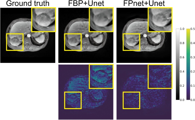
Highlights

• •A learning reconstruction method without using conventional linear reconstructions.
• •Physical model is incorporated in our network structure.
• •Better and more reliable reconstructions.

Abstract

Medical image reconstruction methods based on deep learning have recently demonstrated powerful performance in photoacoustic tomography (PAT) from limited-view and sparse data. However, because most of these methods must utilize conventional linear reconstruction methods to implement signal-to-image transformations, their performance is restricted. In this paper, we propose a novel deep learning reconstruction approach that integrates appropriate data pre-processing and training strategies. The Feature Projection Network (FPnet) presented herein is designed to learn this signal-to-image transformation through data-driven learning rather than through direct use of linear reconstruction. To further improve reconstruction results, our method integrates an image post-processing network (U-net). Experiments show that the proposed method can achieve high reconstruction quality from limited-view data with sparse measurements. When employing GPU acceleration, this method can achieve a reconstruction speed of 15 frames per second.

1. Introduction

Photoacoustic tomography (PAT) is an emerging, fast-developing, and noninvasive biomedical imaging modality that can reveal the optical absorption properties of tissue and molecular probes [1], [2], [3], [4]. In PAT, a short laser pulse illuminates the region of interest in a semi-transparent biological or medical object. The illuminated region absorbs the light energy and converts it into thermal energy, which is ultimately converted into ultrasound by the thermal expansion effect. The induced time-dependent acoustic waves are measured outside the imaging object by transducers. These time-domain signals can be used to restore the initial pressure distribution of the imaging object.

In order to obtain high-resolution reconstructed photoacoustic images, a sufficiently high time/spatial sampling rate and full-view detection geometry are required. Owing to geometrical and cost limitations, it may not be possible for the spatial sampling rate to reach the Nyquist rate, leading to inaccurate reconstructions [5], [6], [7], [8]. On occasion, the spatial sampling rate must be sacrificed in order to accelerate the data acquisition process [9]. In addition to subsampling, limited-view detection, in which the detection surface or curve does not completely surround the imaging target, is also a common occurrence in PAT [10]. The limited-view problem can lead to loss of information, which limits the accuracy and stability of reconstructions [5], [11]. In several PAT imaging systems, suboptimal detection views or limited numbers of transducer locations prevent the system from achieving the desired resolution. PAT reconstruction based on restricted spatial sampling signals with limited-view detection is a problem worth studying.

At present, conventional PAT reconstruction algorithms can be roughly divided into two categories: linear reconstruction methods and model-based reconstruction methods. Linear reconstruction methods mainly include filtered backprojection (FBP) [12], [13], [14], [15] and time reversal [16], [17], [18], which essentially involve solving a single wave equation and obtaining reconstructed images through an approximate linear transformation from the signal domain to the image domain. Thus, these algorithms are computationally efficient and suitable for tasks requiring high time resolution. However, applying these algorithms to subsampled and limited-view data will result in low-quality images with many artifacts [11].

Model-based reconstruction algorithms rely on an optimized iterative strategy to minimize the difference between the measured signal and the predicted signal estimated by the photoacoustic forward model. For accurate reconstruction, model-based reconstruction algorithms require an accurate model matrix and appropriate prior knowledge, referred to as a regularization term. Typical model matrix construction methods include interpolated methods [19], [20] and curve-driven-based methods [21]. Both methods are based on angular discretization of the photoacoustic forward model. The introduction of prior knowledge enables iterative algorithms to reduce artifacts and significantly improve reconstruction quality [5], [22], [23], [24]. However, there is currently no prior knowledge expressed by a regularization term that can fully describe reconstruction results, which can lead to suboptimal results. In addition, model-based reconstruction algorithms are time-intensive, and the weight of the regularization term significantly influences the reconstruction results. These factors restrict the performance of this method.

In recent years, deep learning technology has developed rapidly and has achieved great success in image classification [25], object detection [26], [27], image segmentation [28], [29], and other domains. However, the application of deep learning in PAT reconstruction has only recently emerged [11,[30], [31], [32], [33]]. At present, PAT reconstruction algorithms based on deep learning can generally be classified into two categories.

• 1.Linear reconstruction followed by post-processing. In this strategy, images inaccurately reconstructed by the linear reconstruction method are inputted to a post-processing convolutional neural network (CNN) [30], [31]. The linear reconstruction process can be implemented using a fully connected (FC) network with fixed parameters. In [30], the authors added learnable parameters to a linear reconstruction network to further improve the quality of the images input to the CNN. Hengrong Lan et al. [32] added another encoder for the raw signal to the U-net structure and the reconstructed image was produced by a decoder using joint features of the signal and image. This approach can obtain high reconstruction quality from limited-view data in the line measurement geometry. However, this network cannot generate the correct reconstructed images in our settings, possibly because their network excessively downsamples on the transducer axis, and its concatenation is applied to different domain features with low spatial correlation. Therefore, it is unsuitable for sparsely sampled data in the circular measurement geometry.
• 2.CNN-based iterative network. This type of network was firstly proposed by Andreas Hauptmann et al. [11] in PAT. The network accurately mimics the proximal gradient operator and integrates the learning of prior knowledge. Yoeri E. Boink et al. [33] developed a CNN based on the partially learned algorithm. Their network can achieve image reconstruction and segmentation simultaneously, and is very robust to the image disturbance and different system settings. Unlike the conventional iterative process, this type of network requires a suitable initial value, which is generated by a linear reconstruction algorithm. In this strategy, one-step iteration is equivalent to one network operation with different parameters.

Although all of the aforementioned deep learning reconstruction algorithms can obtain state-of-the-art results, the reconstructions are still highly dependent on the linear reconstruction method. When the signal data is incomplete, the results of the above methods will degenerate, owing to the inferior reconstruction quality of conventional linear reconstruction methods. Ominik Waibel et al. firstly attempted to use CNN to implement the transformation from the signal domain to the image domain [34]. However, the reconstruction quality of this method is lower than that of other deep learning methods, and its effectiveness has not been validated in realistic data reconstructions. In this study, in an effort to improve reconstruction quality in signal-to-image domain transformation, a novel deep learning–based reconstruction approach independent of conventional linear reconstruction algorithms, inspired by the AUTOMAP network [35], is presented. Unlike AUTOMAP, the design of our network structure incorporates the physical model. To the best of our knowledge, this is also the first attempt to use the physical model as the prior information for the network structure in photoacoustic image reconstruction. In our study, the problem has been restricted to sparsely sampled, limited-view PAT reconstruction in circular measurement geometry. The network used for domain transformation is referred to as the Feature Projection Network (FPnet). After a domain transformation is completed, a U-net network further improves the image, as in [30], [31]. Moreover, a data pre-processing method has been designed with training strategies to further improve network performance. Our method can be extended to any two- or three-dimensional measurement geometry. In order to verify the performance of the network, numerical simulations as well as in vivo experiments were conducted.

2. Background

2.1. Photoacoustic tomography

In PAT, the imaging object is illuminated by a short-pulse laser light, and the ultrasonic wave is generated by the thermoelastic expansion effect. When the heat confinement condition is met, the photoacoustic imaging process can be approximated as the following photoacoustic wave equation [21], [20]

$$\frac{{\partial }^{2}p(\text{r},t)}{\partial t^2}-c^2{\nabla }^{2}p(\text{r},t)=\mathrm{\Gamma }H(\text{r})\frac{\partial \delta (t)}{\partial t},$$ (1)

where r and t represent position and time, respectively, δ(t) is the delta function, c is the speed of sound in the medium, Γ is the dimensionless Grüneisen parameter, and H(r) is the initial pressure distribution. The goal of PAT reconstruction is to obtain an accurate initial pressure distribution H(r).

2.2. Universal backprojection

Universal backprojection (UBP) is a linear reconstruction method first proposed by Xu and Wang in 2005 [12]. The discretized UBP euqation is analytically derived from the photoacoustic wave equation (1), which can be written as

$$H(\text{r})=\sum _{i=1}^{N}b\left({\text{d}}_i,t=\frac{|\text{r}-{\text{d}}_i|}{c}\right)\frac{\mathrm{\Delta }{\mathrm{\Omega }}_i}{{\sum }_{i=1}^N\mathrm{\Delta }{\mathrm{\Omega }}_i},$$ (2)

where d_i and ΔΩ_i represent the position and solid angle, respectively, of the ith transducer. b(d_i, t) is the backprojection term and is related to the pressure intensity detected by the ith transducer, which can be written as

$$b({\text{d}}_i,t)=2p({\text{d}}_i,t)-2t\frac{\partial p({\text{d}}_i,t)}{\partial t}.$$ (3)

Clearly, Equation (2) can be written as a linear transformation from the signal domain to the image domain, which is

$$\text{H}=\text{M}\text{b},$$ (4)

where H and b are vectors, and M is the discrete matrix coefficient of (2).

Linear reconstruction based on the discrete UBP equation has proven capable of obtaining exact reconstruction results in case of infinite measurements without noise. In general, UBP still achieves acceptable results with sufficient measurements and limited noise. However, when supplied with limited-view and sparsely sampled signals, the lack of information has a significant negative impact on the reconstruction quality.

2.3. Model-based reconstruction

Model-based algorithms are dedicated to discretizing the forward propagation of photoacoustic signals. For discretization needs, Equation (1) can usually be expressed as an initial value problem. The analytical solution of this initial value problem can be written in matrix-vector product form [19], [21], [20]

$$\text{p}=\text{A}\text{H},$$ (5)

where p is the vector-form signal, H is the vector-form initial pressure distribution, and A is the discretized forward model matrix. However, solving (5) directly is time-consuming and unrealistic owing to the vast dimension of model matrix A. Therefore, the iterative method based on optimization is a better choice. In general, another regularization term is required to induce the prior knowledge about the structure of reconstructed images. The optimization problem based on standard Tikhonov and TV regularization can be written as (6) and (7)

$${\text{H}}_{\mathrm{sol}}=\underset{\text{H}}{argmin}\left\{\Vert \text{p}-\text{A}\text{H}{\Vert }_2^2+\lambda \Vert \text{H}{\Vert }_2^2\right\},$$ (6)

$${\text{H}}_{\mathrm{sol}}=\underset{\text{H}}{argmin}\left\{\Vert \text{p}-\text{A}\text{H}{\Vert }_2^2+\lambda \Vert \nabla \text{H}{\Vert }_1\right\},$$ (7)

where λ is the regularization parameter.

By employing iterative optimization strategies in conjunction with prior information, iterative methods can often achieve better reconstruction results than linear reconstruction methods. However, no regularization term can fully describe the actual situation, which limits the quality of reconstructed images. In the case of limited-view and sparsely sampled measurements, the optimization problem becomes ill-posed, further limiting the performance of such methods. Moreover, because of its iterative processing, this type of method has relatively high computational complexity.

2.4. U-net based reconstruction

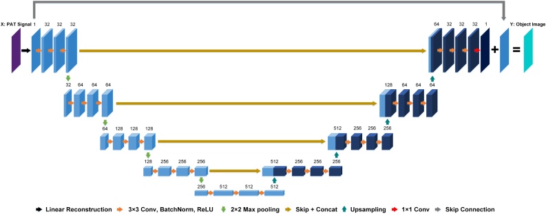
The U-net structure was first proposed for medical image segmentation [29]. In the field of medical image reconstruction, a U-net is typically used to denoise the reconstruction results from linear reconstruction methods [31], [30], [25]. In [36], the authors first integrated the idea of residual learning into U-net. They found that it was easier for the U-net to learn the image artifact pattern than to directly learn a denoising process. Implementing the residual learning strategy can further improve denoising performance. Fig. 1 shows the architecture of the U-net with the residual learning strategy for PAT reconstruction. Although the U-net is widely used in image post-processing, it may not be the best network. Daniël Pelt [37] proposed a mixed scale and densely connected CNN. They replaced the pooling layer with the dilation convolutions and make the network adaptively learn the combination of the dilation size. Their approach is able to achieve accurate results with fewer parameters than the U-net in medical image denoising. This method has given us a good inspiration and we will design a better image post-processing network with fewer parameters for PAT in our future work.

Fig. 1.

U-net structure with residual learning strategy for PAT reconstruction. The number written above each layer represents the number of filters, which is also equivalent to the number of feature maps. The linear reconstruction portion (black arrow) can be implemented outside the U-net using conventional methods or integrated by a fully connected network with fixed parameters preceding the U-net.

3. Proposed Method

3.1. Data pre-processing

In this study, as the first step, a nonlinear transformation was proposed to normalize the signal data. It can be written as follows:

$$\tilde{\text{p}}(i)=2\frac{\text{p}(i)-min(\text{p})}{max(\text{p})-min(\text{p})}-1,$$ (8)

where p is one signal sample, p(i) is the ith element of the original signal, and $\tilde{\text{p}}(i)$ is the ith element of the corresponding transformed signal. After this transformation, the single signal sample has a maximum value of 1 and a minimum value of -1, because simulated signals include both negative and positive values. The only difference between this nonlinear transformation and a conventional linear transformation is that only single-sample statistics are used, rather than the statistics of the entire dataset. The reasons for using the nonlinear transformation are as follows: 1) The distribution of simulated signals is different from the distribution of realistic signals obtained by the PAT system, and statistical information that satisfies both simulated and realistic signals cannot be obtained; 2) The above transformation does not change the reconstruction results of any conventional reconstruction algorithms when all reconstructed images are normalized to [0, 1] using the same transformation.

In Supplementary Material Section S.I, we briefly explain these two reasons and discuss the feasibility of this nonlinear transformation.

3.2. Feature Projection Network for domain transformation

In this study, we propose the Feature Projection Network (FPnet), a novel network architecture for signal-to-image domain transformation. Unlike other PAT reconstruction networks [31], [30] that rely on conventional linear reconstruction methods or fully connected (FC) layers with fixed parameters to perform domain transformation, FPnet directly learns domain transformation through a data-driven approach. It contains several convolutional layers for feature extraction, one max pooling layer for downsampling, and one FC layer for domain transformation. The proposed FPnet is illustrated in Fig. 2A, inside the dotted box.

Fig. 2.

Schematic of the proposed network. (A) Architecture of FPnet with the U-net as a post-processing network. FPnet (inside the dotted box) is used to implement the signal-to-image domain transformation. The U-net is used to further fix the reconstructed image obtained from FPnet. The numbers above each layer indicate the size of the feature map as (height × weight × channel). (B) Residual block used in FPnet.

The architecture in this study is motivated by the UBP equation and the AUTOMAP network for domain transformation [35]. Our basic idea is to integrate the photoacoustic physical model into our network structure as prior information. From (2) and (3), it can be seen that the signal p(d_i, t) and the first-order partial derivative of the signal versus time $\frac{\partial p({\text{d}}_i,t)}{\partial t}$ have a critical impact on the initial pressure reconstruction. According to this feature, our proposed FPnet also has dual inputs, named as, the normalized signal and the time derivative of the normalized signal. The central difference was used to approximate the time derivative in our study. It can be written as

$$\frac{\partial p({\text{d}}_i,t)}{\partial t}\approx \frac{p({\text{d}}_i,t+\mathrm{\Delta }t)-p({\text{d}}_i,t-\mathrm{\Delta }t)}{2\mathrm{\Delta }t}.$$ (9)

To the best of our knowledge, the FC layer is a feasible structure that can learn a transformation from the signal domain to the image domain. Examples of domain transformation networks can be found in [35] and [38]. However, the dimension for PAT signals is very large (usually a vector of over 50000 double-precision elements), resulting in an excessive number of parameters, if the domain transformation is directly implemented using one or more FC layers. Therefore, it is unrealistic to directly use FC layer(s) for domain transformation of these two inputs, owing to the limitations of the computational capability of the hardware. This is also one of the biggest challenges of applying a deep learning-based approach for direct signal-to-image domain transformation in PAT reconstructions.

In order to solve this problem, some noncritical signals are first removed. The principle of truncation is to retain only the signal in the valid period. For every ultrasound transducer, there is a valid period including all sampling moments t that approximately satisfy the following relationship

$$t\in \left[\frac{L_{min}}{c},\frac{L_{max}}{c}\right],$$ (10)

where L_min and L_max are the minimum and maximum distance between the transducer and the imaging pixel. This data truncation strategy was inspired by the process of establishing the model matrix in [20], [19], [21]. When discretizing the forward model, a basic assumption is that the initial pressure generated outside the imaging field of view (FOV) does not contribute to the signal intensity.

After the signal data is truncated, in order to further overcome the problem of excessive parameters caused by directly using FC layers, the convolutional layers are used first to extract the features from the signal. Before convolution, the signal is expanded into a matrix, where the rows represent the transducers and the columns represent the times. Then, 1 × 15 convolutional layers with a residual block structure [25] (Fig. 2B) are used for feature extraction. It should be noted that we only convolve on the time axis, because in the sparse sampling problem, the transducers are not close to each other, and the correlation between signals of adjacent channels is relatively low. The size of the convolution kernel is not arbitrarily determined; rather, it is based on the discrete process of the photoacoustic forward model, which is explained in detail in Supplementary Material Section S.II.

Similar to other networks, two sets of three residual blocks are utilized to expand the receptive field and extract deeper features, and one max pooling layer is used to downsample and retain the main features. The same operation is performed on the dual inputs. The two sets of feature maps are summed into one set of feature maps, and subsequently these feature maps are further processed by three residual blocks. Finally, only one FC layer is used to project the signal features into the image domain. The domain transformation learned by FPnet is

$${\text{H}}_f=\mathcal{F}\left({\mathcal{C}}_2\left({\mathcal{C}}_0\left(p({\text{d}}_i,t)\right)+{\mathcal{C}}_1\left(\frac{\partial p({\text{d}}_i,t)}{\partial t}\right)\right)\right),$$ (11)

where ${\mathcal{C}}_0$, ${\mathcal{C}}_1$, and ${\mathcal{C}}_2$ are the feature-extraction networks for p(d_i, t), $\frac{\partial p({\text{d}}_i,t)}{\partial t}$, and the summed feature map, respectively, and $\mathcal{F}$ is the FC layer for domain transformation. The above learning process can be considered as learning a more accurate UBP equation (2). The difference is that we first use the convolutional layers to extract the features of the signal, and then use one FC layer to learn a domain transformation matrix for transforming signal features to images. The advantage of using the convolutional layers to extract signal features is that such a strategy effectively utilizes the strong correlations between signals at adjacent moments and can effectively reduce the number of FC layers while significantly reducing the number of parameters.

3.3. Instance normalization

The normalization layer used in residual blocks (Fig. 2B) of the proposed FPnet is based on instance normalization (IN) instead of batch normalization (BN). IN was first proposed by Dmitry Ulyanov et al. for image stylization [39]. It applies normalization to each channel of a feature map, which does not involve the statistics of mini-batch data. Owing to the nonlinear normalization, BN cannot obtain correct statistical information from the training dataset, which leads to unreliable test results. The IN normalization is similar to the nonlinear transformation proposed in Section 3.1. From another perspective, the nonlinear normalization method is also a different form of IN. Therefore, using IN instead of BN can improve network performance and accelerate the convergence of the network. In Supplementary Material Section S.VIII, we further verified the effectiveness of IN through experiments.

3.4. Post-processing network

Although FPnet can produce reconstructed images far more accurately than the convolutional linear reconstruction method, pixels of images outputted by one FC layer are not sufficiently stable. Thus, a post-processing network can be utilized to further improve reconstruction quality. To ensure a fair comparison in experiments, we also use the U-net architecture in Fig. 1 for post-processing. Therefore, the complete network (Fig. 2) for our method includes a FPnet for domain transformation and a U-net for post-processing.

3.5. Guided learning strategy

To effectively train the network, a novel training strategy referred to as the Guided Learning Strategy (GLS) is presented to simultaneously train FPnet and U-net. The core of the proposed GLS is the design of the loss function, which is

$$\begin{array}{cc}\hfill \mathrm{Loss}& =\alpha {\mathrm{Loss}}_f+{\mathrm{Loss}}_u\hfill \\ \hfill & =\alpha \mathrm{MSEloss}({\text{H}}_f,{\text{H}}_{\mathrm{gt}})+\mathrm{MSEloss}({\text{H}}_u,{\text{H}}_{\mathrm{gt}}),\hfill \end{array}$$ (12)

where Loss_f is the mean square error loss (MSEloss) between the output of FPnet H_f and the ground truth H_gt, Loss_u is the MSEloss between the output of the U-net H_u and the ground truth H_gt, and α is a scale factor. Because this network was designed to learn a more accurate domain transformation instead of relying on image post-processing, α > 1 is necessary. The design of this weighted multipart loss function was inspired by Faster RCNN [27]. In this study, α is set to 10 based on the convergence speed and reconstruction quality of FPnet. In Supplementary Material Section S.III, the experiments for selecting α are discussed in detail.

According to our loss function, the gradient update process of FPnet and the U-net can be written as

$$\begin{array}{cc}\hfill {\omega }_f& ={\omega }_f-\mu \left(\alpha \frac{\partial {\mathrm{Loss}}_f}{\partial {\omega }_f}+\frac{\partial {\mathrm{Loss}}_u}{\partial {\omega }_f}\right)\hfill \\ \hfill {\omega }_u& ={\omega }_u-\mu \frac{\partial {\mathrm{Loss}}_u}{\partial {\omega }_u}\hfill \end{array},$$ (13)

where ω_f denotes the parameters of FPnet and ω_u denotes the parameters of U-net; μ is the learning rate. The U-net parameters will only be affected by the gradient backpropagation from Loss_u, such that the U-net can learn how to improve the image quality outputted by FPnet. The update of the FPnet parameters can be considered as a two-step process. First, the parameter update is performed by the gradient backpropagation from Loss_f, resulting in a more accurate domain transformation. Then, in order to fine-tune the parameters, they are updated by the gradient backpropagation from Loss_u. As a result, the image reconstructed by FPnet can better adapt to the denoising performance of the U-net network. Because we set α > 1, the first step plays an important role.

Because of the large number of FC layer parameters, our method must consider the problem of overfitting, which will persist when simply using the loss function to guide network training. Therefore, L1 regularization is used here to constrain the parameter value of the FC layer. This was inspired by the discretized UBP equation (2), in which the initial pressure intensity of a reconstructed point only contains the contributions from the signal magnitudes of few moments at each transducer. This is consistent with the feature selection function of L1 regularization. Therefore, it can assumed that only a small portion of the signal features extracted by the convolution network in FPnet will be particularly important for a reconstructed pixel. The final loss function of GLS including L1 regularization term is written as

$$\mathrm{Loss}=\alpha \mathrm{MSEloss}({\text{H}}_f,{\text{H}}_{\mathrm{gt}})+\mathrm{MSEloss}({\text{H}}_u,{\text{H}}_{\mathrm{gt}})+\gamma |{\omega }_f{|}_1,$$ (14)

where γ is the L1 weight decay value.

In short, we designed a loss function that guides the network which prefers to learn a more accurate feature projection rather than rely heavily on post-processing. Moreover, the overfitting was suppressed by using a regularization strategy to limit the value and sparsity of FC layer parameters.

4. Experiments and Discussions

Numerical simulations and in vivo experiments were conducted in order to verify the performance of the proposed reconstruction method. Both qualitative and quantitative analyses were employed to illustrate the superiority of our method.

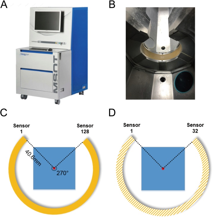
Most of the experimental settings were based on those of the MSOT inVision 128, a commercial small animal PAT imaging system (iTheraMedical GmbH, Neuherberg, Germany, Fig. 3A). In this system, the circular transducer contains 128 detection elements and covers an angle of 270^∘ around the imaging object at a sampling frequency of 40 MHz (Fig. 3B and C). Obviously, this imaging system will encounter the limited-view problem. To further simulate the subsampling situation, the number of transducers was uniformly downsampled four times (Fig. 3D). The 32-channel signal was used as a subsampled signal, and the original 128-channel signal was used as a fully sampled signal.

Fig. 3.

Experimental equipment and detector. (A) MSOT inVision 128 imaging system. Most experimental settings in this study were consistent with those used in this system. (B) Photograph of circular transducer in this system. (C) Schematic of the transducer. (D) Schematic of the downsampling scenario in our experiments. In this study, the number of transducers was uniformly downsampled four times. The 32-channel signal was used as a subsampled signal, and the original 128-channel signal was used as a fully sampled signal.

The training and validation of our network were implemented via PyTorch in Python, using two Titan Xp GPUs with 12 GB memory. All test results were obtained using a PC with six 3.7 GHz processors and 32 GB of memory.

4.1. Dataset and network training

In numerical simulations, four datasets containing different structural features were used to verify the performance of our method and the baseline methods. In Fig. 4, some example images are shown for visual display. The Vessel dataset was obtained by randomly cropping the images from the DRIVE dataset which contains retinal blood vessel images [40]. In order to increase the complexity of images in the Vessel dataset, background intensity and random perturbations of both background and vessels were added to each image. The Brain dataset is a publicly available MRI brain dataset which can be downloaded from the website of The Cancer Imaging Archive (TCIA)² [41]. Both the Abdomen and LiverCancer datasets consist of abdomen MRI images and were provided by the First Affiliated Hospital, Jinan University. The Abdomen dataset was used for training and testing, and all images were from healthy people. In contrast, all the images in the LiverCancer dataset contained tumors from liver cancer patients. The LiverCancer dataset was not used for training and was only a test dataset for the network trained on the Abdomen dataset. This dataset was used to test the performance of our method for reconstructing the pathologies which are not represented in the training data. The signal data was obtained by p = AH, where A is the model matrix in [20]. In the training process, Gaussian noise with random intensity was added to the simulated signal, resulting in a wide range of signal-to-noise ratios (SNR) from 10 dB to 40 dB. Therefore, the final simulated signal can be indicated as p_n = p + g, where g is the Gaussian noise. All images were converted to a size of 128 × 128 with a grid spacing of 200 μm. All other experimental settings were in accordance with the MSOT inVision 128 system. Table 1 presents a brief explanation of each dataset and gives the number of training, validation, and test samples.

Fig. 4.

Example of images in each dataset used in numerical simulations. See Table 1 for detailed information.

Table 1.

Description of each dataset used in numerical simulations and in vivo experiments.

Dataset	Explanation	Training samples	Validation samples	Test samples
Brain	Brain MRI images of T1-weighted post-contrast, FLAIR and T2-weighted imaging.	2211	267	276
Abdomen	Abdomen MRI images of T1-weighted post-contrast imaging from healthy people.	8273	368	336
Vessel	Vessel images that is randomly cropped from the DRIVE dataset.	4000	200	200
LiverCancer	Abdomen MRI images of T1-weighted post-contrast imaging from liver cancer patients.	-	-	601
MSOT-Brain	Brain PAT images of nude mice extracted from the MSOT InVision 128 system.	698	-	64
MSOT-Abdomen	Abdomen PAT images of nude mice extracted from the MSOT InVision 128 system.	575	-	124

To relieve overfitting and accelerate network convergence, we first performed 20 epochs of pre-training using 15000 natural images (and their corresponding simulated PAT signals) from the PASCAL VOC2012 dataset [42] (see the experiments about the improvement of using pertraining in Supplementary Material Section S.VIII). Then, each dataset was used to train another 50 epochs. We trained our network using PyTorch's implementation of the Adam optimizer [43] with a batch size of 24. Learning rates of 10⁻⁴ were employed for pre-training and 10⁻⁵ for further training. The FC layer was initialized by Xavier uniform initializer with a gain value of 0.1 and the L1 weight decay value was set to 10⁻⁶.

In in vivo experiments, we established two datasets named MSOT-Brain and MSOT-Abdomen, which contain realistic signals and corresponding reconstructed images extracted from the MSOT inVision 128 system with some additional pre-processing. Owing to the limited number of in vivo data, all these datasets do not include validation samples. The images in the training set and the test set are from different scans and mice. The data extraction process and pre-processing method are described in detail in Supplementary Material Section S.IV. These data enable the network to extract features from realistic signals. It should be noted that these reconstructed images used as ground truth images were obtained by the model-based reconstruction algorithm included in the system software. Although this system can achieve reliable reconstructions, these images are not the real ground truth. For practical applications, it is sufficient to learn the reconstructed results of a commercially available system under the fully sampled condition. The detailed information about these two datasets is presented in Table 1. For in vivo experiments, the size of FOV was 25 mm × 25 mm, and the reconstructed images were converted to the same size as the images in simulated datasets. The training rules of the in vivo experiments were the same as those in the numerical simulations.

The data pre-processing for all numerical simulations and in vivo experiments was based on the nonlinear transformation method proposed in Section 3.1. Every sample in all datasets was consistent with (p, H_gt), where p is the simulated signal with Gaussian noise in numerical simulations or the realistic signal in in vivo experiments, and H_gt is the ground truth of the initial pressure distribution.

In the following content, FPnet+Unet are used to represent the method proposed in this paper, and FPnet is used to represent reconstructions produced solely by FPnet, without using U-net.

4.2. Baseline algorithms

This study utilized standard Tikhonov reconstruction, TV reconstruction and Filtered Backprojection (FBP) with U-net post-processing as baseline algorithms. Hereafter, we used Tikhonov, TV and FBP+Unet to represent these three methods. All algorithms are briefly discussed in Section 2. For standard Tikhonov reconstruction, LSQR algorithm were used for iterative updates [44]. The number of iterations used for LSQR is 100. For TV reconstruction, we used the split Bregman method employed in [45] to solve (7) with 50 Bergman iterations. The regularization parameter of these two model-based methods were set to a relative optimal value according to the experiments (see Supplementary Material Section S.V). To ensure a fair comparison, the training parameters and datasets used for FBP+Unet were the same as that used for FPnet+Unet, except that the learning rate was constant at 10⁻⁴ and the batch size was 64.

In addition, in order to verify the reconstruction performance of the proposed FPnet and the functionality of the U-net in FPnet+Unet, we also added FBP and FPnet to the baseline algorithms. The implementation of the FBP algorithm was based on [12].

4.3. Performance metrics

To quantitatively illustrate the quality of the reconstructed images, we used normalized root mean-squared error (NRMSE), peak-signal-to-noise ratio (PSNR), and structure similarity (SSIM) [46] as metrics. The calculation of these quantitative indicators was implemented using the scikit-image package in Python. During the quantitative analysis of the reconstructed images, we also considered the reconstruction time (see Supplementary Material Section S.VII).

4.4. Numerical simulations

In numerical simulations, reconstruction performance and robustness of our method were tested. On the other hand, in order to further verify the theoretical feasibility of our method in biomedical applications, we also tested the accuracy of reconstructions for the pathological features which are not included in the training set.

4.4.1. Reconstruction performance

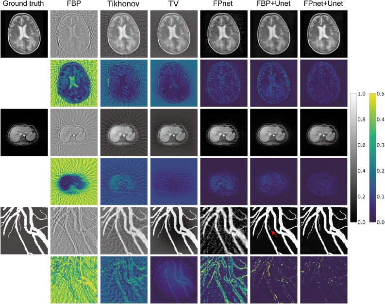
For both FBP+Unet and FPnet+Unet, we trained and tested three models based on the Brain, Abdomen and Vessel datasets, respectively. Without loss of generality, all baseline algorithms and our method were tested on the samples with 20 dB SNR. In Fig. 5, it can be found that the results of deep learning–based methods (FBP+Unet and FPnet+Unet) are generally better than others. Moreover, FPnet+Unet obtained the best reconstructions for the initial pressure intensity on all datasets. At the same time, FPnet+Unet restored detailed structure (e.g. vessels) with higher quality than FBP+Unet. The blood vessel indicated by the red arrow in Fig. 5, all methods except for FBP+Unet was successfully reconstructed. Although FBP successfully reconstructed this blood vessel, the U-net failed to reconstruct it owing to the interference of artifacts in the FBP images. Based on more accurate and reliable domain transformation of FPnet, FPnet+Unet obtained higher quality results. In addition, it should be noted that the artifacts generated in FPnet were similar to the subsampled artifacts in FBP and Tikhonov methods (especially in the Vessel dataset), which proved that we incorporated the prior knowledge of UBP physical model into the network structure. The quantitative measurements are shown in Table 2. These results further revealed that our method achieved the best performance in all quantitative indicators.

Fig. 5.

Performance comparisons for three test images from the Brain, Abdomen and Vessel datasets, respectively (from top to bottom). Gray-scale images demonstrated the ground truth and corresponding reconstructed results produced by each method. Pseudo-color images are the subtraction between the reconstructed results and ground truth.

Table 2.

Mean PSNR, SSIM and NRMSE of noisy test samples for Brain, Abdomen and Vessel datasets.

Dataset		FBP	Tikhonov	TV	FPnet	FBP+Unet	FPnet+Unet
Brain	PSNR	9.9428	17.8090	20.8906	25.7187	26.5650	27.6908
	SSIM	0.2862	0.4807	0.6139	0.7385	0.7972	0.8620
	NRMSE	1.2468	0.5245	0.3756	0.2034	0.1846	0.1630
Abdomen	PSNR	7.5409	18.1119	19.5252	29.1673	30.7155	31.3335
	SSIM	0.1379	0.2504	0.3024	0.8349	0.8430	0.8852
	NRMSE	2.3025	0.6965	0.5944	0.1947	0.1606	0.1498
Vessel	PSNR	8.0661	16.6168	22.9560	16.4563	21.6138	25.1170
	SSIM	0.1356	0.4223	0.8300	0.3975	0.8690	0.9059
	NRMSE	1.2164	0.4630	0.2297	0.4597	0.2566	0.1714

4.4.2. Robustness against noise

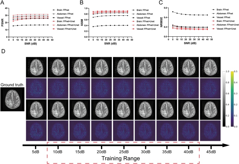
The robustness was tested against different noise levels for FPnet+Unet. For the Brain, Abdomen and Vessel test sets, we generated noisy signals from 5 dB to 45 dB SNR with a 5 dB step. It should be noted that the 5 dB and 45 dB SNRs were not included in the training samples, which can further illustrate the robustness against stronger or weaker noise without training. In this experiment, three models were also trained and tested on the corresponding test samples. It can be seen from Fig. 6A-C that both FPnet and FPnet+Unet were generally robust against noise. Even the SNR of the signal outside the training set, FPnet+Unet can still achieve acceptable results. It should be noted that when the noise is strong (less than 20 dB SNR), the network performance will slightly reduce owing to the more unstable intensity of the reconstructed images generated by FPnet. However, in Fig. 6D, the slight decrease in quantitative indicators has almost negligible effect on the visual impression of reconstructions. Also, a better reconstruction for a signal with certain intensity noise can be obtained by narrowing the noise range of the training set. In total, it can be found that both FPnet and FPnet+Unet were well applied to noise situations.

Fig. 6.

Robustness against different SNRs. (A-C) Mean PSNR, SSIM, NRMSE of the test images generated by FPnet and FPnet+Unet in the Brain, Abdomen and Vessel dataset versus SNRs. The black and red color indicate FPnet and FPnet+Unet, respectively. (D) Visual display of one set of reconstruction result with different SNRs in the Brain dataset. Gray-scale images demonstrated the ground truth and corresponding reconstructed results produced by FPnet (first row) and FPnet+Unet (third row). Pseudo-color images are the subtraction between the reconstructed results and ground truth.

4.4.3. Robustness against pathologies

In biomedical application, it is a very common phenomenon to detect pathological features not found in the training set. Therefore, it is necessary to test the ability to reconstruct the pathological features not contained in the training set. In this experiment, the model trained on the Abdomen dataset was used and tests were conducted on samples with 20 dB SNR in the LiverCancer dataset. All the features of liver tumors were not learned by both FBP+Unet and FPnet+Unet. An example of reconstructions using deep learning–based methods is shown in Fig. 7. It can be seen that the accuracy of the initial pressure reconstruction was significantly higher than that from FBP+Unet. In addition, FPnet+Unet obtained more reliable reconstruction for pathologies which were not represented in the training data. This is mainly reflected in the more accurate reconstructions of the initial pressure of liver tumor and its peritumoral vessels. This more accurate result is mainly due to the fact that our network structure combined the physical model and learned a more reliable domain transformation under data-driven conditions. In the quantitative measurements (Table 3), although the SSIM of both methods were similar, the PSNR and NRMSE of FPnet+Unet were significantly higher than FBP+Unet, which further demonstrated that FPnet+Unet can obtain higher reconstruction quality on the pathological features without training. For FPnet itself, it was still possible to reconstruct the pathological features not included in the training set with high quality. This is the root cause of FPnet+Unet surpassing FBP+Unet. In general, FPnet+Unet was still robust to pathological features not represented in the training set, and its reconstruction results were reliable.

Fig. 7.

The reconstruction result of a test sample in the LiverCancer dataset. Both FBP+Unet and FPnet+Unet were trained on the Abdomen dataset. Gray-scale images demonstrated the ground truth and corresponding reconstructed results produced by FBP+Unet and FPnet+Unet. Pseudo-color images are the subtraction between reconstructed results and the ground truth. For each result, the image inside the large yellow rectangle is an enlargement of the area inside the small yellow rectangle, intended to show the reconstruction details of the liver tumor more clearly.

Table 3.

Mean PSNR, SSIM and NRMSE of noisy test samples for LiverCancer dataset. Models were trained on the Abdomen dataset.

Algorithm	FPnet	FBP+Unet	FPnet+Unet
PSNR	27.0826	27.1701	28.7152
SSIM	0.8480	0.8940	0.8953
NRMSE	0.1910	0.1883	0.1550

4.5. In vivo experiments

In practice, a signal also contains Gaussian white noise, echo noise, and noise caused by the motion of the imaging object. Therefore, to further verify the robustness and practicality of different reconstruction methods, the data of in vivo photoacoustic mice imaging were adopted for comparison.

In order to accommodate the size of FOV in the commercial imaging system, the pixel spacing settings of FBP, Tikhonov, and TV were adjusted slightly. Here, the default reconstructed images given by the MSOT inVision 128 system were used as the ground truth for the fully sampled, limited-view data. A comparison of different reconstructions from six methods is shown in Fig. 8. In these realistic PAT imaging cases, because of the limited-view signal with sparse sampling, reconstructions produced by FBP and Tikhonov were obviously polluted by strong artifacts. TV over-suppressed these artifacts and caused excessively smooth images. FPnet produced distinctly better results with less artifacts, which was because the network captured key features from the realistic ultrasound signal, and thus produced projections more accurately than the FBP did. Both FBP+Unet and FPnet+Unet achieved more accurate reconstructions than FPnet alone. However, FPnet+Unet was more effective in suppressing the background noise, leading to better overall image quality compared to FBP+Unet. In addition, it is found that FPnet+Unet outperformed FBP+Unet in the reconstruction of small blood vessels in the brain. It should also be noted that for the superficial inferior epigastric vessel (the vessel indicated by the red arrow in the ground truth image) of nude mice, only FPnet and FPnet+Unet were successfully reconstructed, and other methods failed to reconstruct owing to the subsampled measurements, which further demonstrated the reliability of our method for limited-view and sparsely sampled data. Moreover, just like numerical simulations, the subsampling artifact pattern generated by FPnet was similar to conventional methods, which confirmed the use of the physical model as prior information.

Fig. 8.

Performance comparisons for two test images from the MSOT-Brain and MSOT-Abdomen datasets, respectively (from top to bottom). The red arrow points to a superficial inferior epigastric vessel.

A quantitative analysis of test samples from the realistic test sets is shown in Table 4. Our method still outperformed all the other methods in these three indicators, which was consistent with numerical simulations. However, for the MSOT-Brain dataset, it was noted that the difference between FPnet+Unet and FBP+Unet became smaller in comparison with simulation experiments (Table 4). This was because in vivo brain images had a larger background portion, and therefore, it was easier for our network to overfit these smooth background pixels and produced an excessively smooth reconstruction, resulting in degeneration. Another reason was that, the training set was not large enough to optimize all parameters of our network, which also affected its overall performance. Despite this, our method still accurately reconstructed most of the small details in the PAT images (Fig. 8).

Table 4.

Mean PSNR, SSIM and NRMSE of test samples for MSOT-Brain and MSOT-Abdomen datasets.

Dataset		FBP	Tikhonov	TV	FPnet	FBP+Unet	FPnet+Unet
MSOT-Brain	PSNR	20.0477	21.3913	20.1634	26.0701	27.5415	27.9293
	SSIM	0.2670	0.3556	0.6747	0.7656	0.8601	0.8647
	NRMSE	0.2365	0.2198	0.2512	0.1235	0.1055	0.1014
MSOT-Abdomen	PSNR	16.0532	16.1707	15.1748	29.2176	27.3271	30.3972
	SSIM	0.2647	0.3536	0.5404	0.8572	0.8630	0.9073
	NRMSE	0.4771	0.4703	0.5203	0.1042	0.1310	0.0910

5. Conclusions

In this study, a novel deep learning strategy was developed for PAT reconstructions from limited-view and sparsely sampled data. Unlike other deep learning algorithms developed for PAT, our method learned a feature projection process instead of using conventional linear reconstruction methods for domain transformation. When combined with a post-processing network, our method can obtain better results than baseline algorithms.

The effectiveness of this method is primarily due to the following four points. First, the proposed FPnet is able to extract the deep features of the raw signal on the time axis and learn adaptive feature projection parameters on the basis of the training data. Conventional linear reconstruction methods often ignore the correlation between adjacent time signals, resulting in information loss. In the conventional backprojection process, the projection term is highly correlated with the signal at a fixed moment, and as a result, the parameters of the backprojection matrix are also fixed. This inevitably leads to significant inaccuracy, because the actual situation (e.g. the speed of sound) often does not precisely match the ideal assumption. However, this drawback was effectively overcome by the proposed FPnet. Second, the design of FPnet integrated the physical model of the UBP. Although it did not replicate any conventional linear reconstruction algorithms, the fundamental physical model was adopted as the prior knowledge to the network, which improved the reconstruction performance. We believe that implementing a deep learning network without considering the physical principle of photoacoustic imaging is unlikely to achieve accurate reconstruction results. In order to bring our model closer to the backprojection model and reduce overfitting, we added the L1 regularization to the FC layer of FPnet. Through the parameter analysis experiments (see Supplementary Material Section S.VI), we found that FPnet successfully learned a projection process in a manner very similar to UBP. Third, a suitable data pre-processing and training strategy was presented for FPnet+Unet to further improve the reconstruction performance. For data pre-processing, we proposed a nonlinear transformation, which enables the network to cope with different distributions of signals. The GLS was proposed to train FPnet and U-net simultaneously. By increasing the weight of the loss function of output from FPnet, the network focused on the learning of domain transformation. Moreover, by analyzing gradient backpropagation, FPnet adjusted its own parameters according to the image post-processing network, so that it adapted to the denoising performance of the post-processing network. Finally, the convolutional layer and pooling layer were used to extract and downsample features, respectively, which remarkably reduced the number of learnable parameters. This facilitated the efficient implementation of deep learning network.

Certain limitations and potential biases may exist in our study. First, our reconstruction speed was slower than that of FBP+Unet, because the convolutional layer was used to extract features. However, our approach was faster than the iterative reconstruction method and can achieve real-time reconstruction if GPU acceleration can be applied. Second, although the UBP physical model was used as prior information for the FPnet structure, this does not mean that FPnet can learn a universal and real physical model. This is mainly due to the fact that the real physical model is highly complicated and theoretically requires a vast number of samples for training. However, in our approach, it is feasible to learn a better UBP-like projection for a specific imaging region or object. Experiments have shown that the reconstruction results of a specific region learned from a small dataset were reliable. Third, the size of the reconstructed images is limited by the very large number of parameters in the FC layer and weaken the practicability of our method. However, this weakness can be overcome by using GPUs with larger memory. Finally, the use of nonlinear normalization may lead to the loss of quantitative information in the reconstruction results, hindering the application of our method in quantitative imaging.

In future research, we will study the learning of more general physical models, construct larger and higher quality in vivo datasets, design better post-processing networks for FPnet and further optimize our method to make it reliable for photoacoustic quantitative imaging.

Funding

This work was supported by Ministry of Science and Technology of China under Grant No. 2017YFA0205200, 2017YFA0700401, 2016YFC0103803, National Natural Science Foundation of China under Grant No. 61671449, 81227901, and 81527805, Chinese Academy of Sciences under Grant No. GJJSTD20170004, KFJ-STS-ZDTP-059, YJKYYQ20180048, QYZDJ-SSW-JSC005, and XDBS01030200.

Conflict of Interest statement

The authors declare that there are no conflicts of interest.

6. Open Access to the Datasets and Source Code

All the datasets used in our study and the source code of FPnet are open access. You can download them from http://www.radiomics.net.cn/post/132.

Biographies

Tong Tong was graduated from University of Electronic Science and Technology of China and now is a Ph.D candidate from the Institute of Automation, Chinese Academy of Sciences and School of Artificial Intelligence, University of Chinese Academy of Sciences. His major is medical imaging reconstruction and pattern recognition.

Wenhui Huang, a Ph.D candidate from College of Medicine and Biological Information Engineering, Northeastern University. Her major is medical imaging and she mainly focuses on molecular imaging of head and neck tumors.

Dr. Kun Wang is a professor at the CAS Key Laboratory of Molecular Imaging, Institute of Automation, Chinese Academy of Sciences. His research focuses on optical multimodality molecular imaging, including ultrasound radiomics, optical scattering tomography, and photoacoustic tomography. He has published more than 60 papers in SCI journals such as Gut, Advanced Materials, Nature Communications, Optica, IEEE Transaction on Medical Imaging.

Zicong He, graduated from Zhengzhou University and now is a postgraduate student of Jinan University, studying on Imaging and Nuclear Medicine.

Lin Yin was graduated from Jilin University and now is a Ph.D student from the Institute of Automation, Chinese Academy of Sciences and School of Artificial Intelligence, University of Chinese Academy of Sciences. Her major is medical imaging reconstruction and pattern recognition.

Dr. Xin Yang is a professor at the CAS Key Laboratory of Molecular Imaging, Institute of Automation, Chinese Academy of Sciences. Her research focuses on optical multimodality molecular imaging and radiomics.

Shuixing Zhang, a leader from medical imaging center of the First Affiliated Hospital of Jinan University, focuses on molecular imaging research about head and neck tumors and has made great contribution in medical imaging.

Dr. Jie Tian is recognized as a pioneer and a leader in China in the field of molecular imaging. In the last two decades, he has developed a series of new optical imaging models and reconstruction algorithms for in vivo optical tomographic imaging, including bioluminescence tomography, fluorescence molecular tomography, and Cerenkov luminescence tomography. Dr. Tian has more than 100 granted patents in China and three patents in the United States. He is the author of over 300 peer-reviewed journal articles, including publication in Journal of Clinical Oncology, Nature Communications, Advanced Materials, Gastroenterology, PNAS, Clinical Cancer Research, Radiology, IEEE Transactions on Medical Imaging, and many other journals, and these articles received about 20,000 Google Scholar citations.

Appendix B. Supplementary Data

The following are the supplementary data to this article:

References

- 1.Ntziachristos V., Razansky D. Molecular imaging by means of multispectral optoacoustic tomography (msot) Chemical reviews. 2010;110(5):2783–2794. doi: 10.1021/cr9002566. [DOI] [PubMed] [Google Scholar]
- 2.Xu M., Wang L.V. Photoacoustic imaging in biomedicine. Review of scientific instruments. 2006;77(4):041101. [Google Scholar]
- 3.Wang L.V. Multiscale photoacoustic microscopy and computed tomography. Nature photonics. 2009;3(9):503. doi: 10.1038/nphoton.2009.157. [DOI] [PMC free article] [PubMed] [Google Scholar]
- 4.Wang K., Chi C., Hu Z., Liu M., Hui H., Shang W., Peng D., Zhang S., Ye J., Liu H. Optical molecular imaging frontiers in oncology: the pursuit of accuracy and sensitivity. Engineering. 2015;1(3):309–323. [Google Scholar]
- 5.Arridge S., Beard P., Betcke M., Cox B., Huynh N., Lucka F., Ogunlade O., Zhang E. Accelerated high-resolution photoacoustic tomography via compressed sensing. Physics in Medicine & Biology. 2016;61(24):8908. doi: 10.1088/1361-6560/61/24/8908. [DOI] [PubMed] [Google Scholar]
- 6.Guo Z., Li C., Song L., Wang L.V. Compressed sensing in photoacoustic tomography in vivo. Journal of biomedical optics. 2010;15(2):021311. doi: 10.1117/1.3381187. [DOI] [PMC free article] [PubMed] [Google Scholar]
- 7.Rosenthal A., Ntziachristos V., Razansky D. Acoustic inversion in optoacoustic tomography: A review. Current medical imaging reviews. 2013;9(4):318–336. doi: 10.2174/15734056113096660006. [DOI] [PMC free article] [PubMed] [Google Scholar]
- 8.Sandbichler M., Krahmer F., Berer T., Burgholzer P., Haltmeier M. A novel compressed sensing scheme for photoacoustic tomography. SIAM Journal on Applied Mathematics. 2015;75(6):2475–2494. [Google Scholar]
- 9.Haltmeier M., Nguyen L.V. Analysis of iterative methods in photoacoustic tomography with variable sound speed. SIAM Journal on Imaging Sciences. 2017;10(2):751–781. doi: 10.1137/21m1463409. [DOI] [PMC free article] [PubMed] [Google Scholar]
- 10.Paltauf G., Nuster R., Burgholzer P. Weight factors for limited angle photoacoustic tomography. Physics in Medicine & Biology. 2009;54(11):3303. doi: 10.1088/0031-9155/54/11/002. [DOI] [PMC free article] [PubMed] [Google Scholar]
- 11.Hauptmann A., Lucka F., Betcke M., Huynh N., Adler J., Cox B., Beard P., Ourselin S., Arridge S. Model-based learning for accelerated, limited-view 3-d photoacoustic tomography. IEEE transactions on medical imaging. 2018;37(6):1382–1393. doi: 10.1109/TMI.2018.2820382. [DOI] [PMC free article] [PubMed] [Google Scholar]
- 12.Xu M., Wang L.V. Universal back-projection algorithm for photoacoustic computed tomography. Physical Review E. 2005;71(1):016706. doi: 10.1103/PhysRevE.71.016706. [DOI] [PubMed] [Google Scholar]
- 13.Burgholzer P., Bauer-Marschallinger J., Gr“un H., Haltmeier M., Paltauf G. Temporal back-projection algorithms for photoacoustic tomography with integrating line detectors. Inverse Problems. 2007;23(6):S65. [Google Scholar]
- 14.Haltmeier M. Inversion of circular means and the wave equation on convex planar domains. Computers & mathematics with applications. 2013;65(7):1025–1036. [Google Scholar]
- 15.Zeng L., Xing D., Gu H., Yang D., Yang S., Xiang L. High antinoise photoacoustic tomography based on a modified filtered backprojection algorithm with combination wavelet. Medical physics. 2007;34(2):556–563. doi: 10.1118/1.2426406. [DOI] [PubMed] [Google Scholar]
- 16.Mast T.D., Souriau L.P., Liu D.-L., Tabei M., Nachman A.I., Waag R.C. A k-space method for large-scale models of wave propagation in tissue. IEEE transactions on ultrasonics, ferroelectrics, and frequency control. 2001;48(2):341–354. doi: 10.1109/58.911717. [DOI] [PubMed] [Google Scholar]
- 17.Cox B.T., Kara S., Arridge S.R., Beard P.C. k-space propagation models for acoustically heterogeneous media: Application to biomedical photoacoustics. The Journal of the Acoustical Society of America. 2007;121(6):3453–3464. doi: 10.1121/1.2717409. [DOI] [PubMed] [Google Scholar]
- 18.Treeby B.E., Cox B.T. k-wave: Matlab toolbox for the simulation and reconstruction of photoacoustic wave fields. Journal of biomedical optics. 2010;15(2):021314. doi: 10.1117/1.3360308. [DOI] [PubMed] [Google Scholar]
- 19.Rosenthal A., Razansky D., Ntziachristos V. Fast semi-analytical model-based acoustic inversion for quantitative optoacoustic tomography. IEEE transactions on medical imaging. 2010;29(6):1275–1285. doi: 10.1109/TMI.2010.2044584. [DOI] [PubMed] [Google Scholar]
- 20.Dean-Ben X.L., Ntziachristos V., Razansky D. Acceleration of optoacoustic model-based reconstruction using angular image discretization. IEEE Transactions on medical imaging. 2012;31(5):1154–1162. doi: 10.1109/TMI.2012.2187460. [DOI] [PubMed] [Google Scholar]
- 21.Liu H., Wang K., Peng D., Li H., Zhu Y., Zhang S., Liu M., Tian J. Curve-driven-based acoustic inversion for photoacoustic tomography. IEEE transactions on medical imaging. 2016;35(12):2546–2557. doi: 10.1109/TMI.2016.2584120. [DOI] [PubMed] [Google Scholar]
- 22.Arridge S.R., Betcke M.M., Cox B.T., Lucka F., Treeby B.E. On the adjoint operator in photoacoustic tomography. Inverse Problems. 2016;32(11):115012. [Google Scholar]
- 23.Huang C., Wang K., Nie L., Wang L.V., Anastasio M.A. Full-wave iterative image reconstruction in photoacoustic tomography with acoustically inhomogeneous media. IEEE transactions on medical imaging. 2013;32(6):1097–1110. doi: 10.1109/TMI.2013.2254496. [DOI] [PMC free article] [PubMed] [Google Scholar]
- 24.Javaherian A., Holman S. A multi-grid iterative method for photoacoustic tomography. IEEE transactions on medical imaging. 2017;36(3):696–706. doi: 10.1109/TMI.2016.2625272. [DOI] [PubMed] [Google Scholar]
- 25.He K., Zhang X., Ren S., Sun J. Deep residual learning for image recognition. Proceedings of the IEEE conference on computer vision and pattern recognition. 2016:770–778. [Google Scholar]
- 26.Redmon J., Divvala S., Girshick R., Farhadi A. You only look once: Unified, real-time object detection. Proceedings of the IEEE conference on computer vision and pattern recognition. 2016:779–788. [Google Scholar]
- 27.Ren S., He K., Girshick R., Sun J. Faster r-cnn: Towards real-time object detection with region proposal networks. Advances in neural information processing systems. 2015:91–99. doi: 10.1109/TPAMI.2016.2577031. [DOI] [PubMed] [Google Scholar]
- 28.Chen L.-C., Papandreou G., Kokkinos I., Murphy K., Yuille A.L. Deeplab: Semantic image segmentation with deep convolutional nets, atrous convolution, and fully connected crfs. IEEE transactions on pattern analysis and machine intelligence. 2018;40(4):834–848. doi: 10.1109/TPAMI.2017.2699184. [DOI] [PubMed] [Google Scholar]
- 29.Ronneberger O., Fischer P., Brox T. U-net: Convolutional networks for biomedical image segmentation. International Conference on Medical image computing and computer-assisted intervention. 2015:234–241. [Google Scholar]
- 30.Schwab J., Antholzer S., Nuster R., Haltmeier M. 2018. Real-time photoacoustic projection imaging using deep learning. arXiv preprint arXiv:1801.06693. [Google Scholar]
- 31.Antholzer S., Haltmeier M., Schwab J. Deep learning for photoacoustic tomography from sparse data. Inverse problems in science and engineering. 2019;27(7):987–1005. doi: 10.1080/17415977.2018.1518444. [DOI] [PMC free article] [PubMed] [Google Scholar]
- 32.Lan H., Jiang D., Yang C., Gao F. 2019. Y-net: A hybrid deep learning reconstruction framework for photoacoustic imaging in vivo. arXiv preprint arXiv:1908.00975. [DOI] [PMC free article] [PubMed] [Google Scholar]
- 33.Boink Y.E., Manohar S., Brune C. A partially-learned algorithm for joint photo-acoustic reconstruction and segmentation. IEEE transactions on medical imaging. 2019;39(1):129–139. doi: 10.1109/TMI.2019.2922026. [DOI] [PubMed] [Google Scholar]
- 34.Waibel D., Gr”ohl J., Isensee F., Kirchner T., Maier-Hein K., Maier-Hein L. Reconstruction of initial pressure from limited view photoacoustic images using deep learning. Photons Plus Ultrasound: Imaging and Sensing 2018, Vol. 10494. 2018:104942S. [Google Scholar]
- 35.Zhu B., Liu J.Z., Cauley S.F., Rosen B.R., Rosen M.S. Image reconstruction by domain-transform manifold learning. Nature. 2018;555(7697):487. doi: 10.1038/nature25988. [DOI] [PubMed] [Google Scholar]
- 36.Han Y.S., Yoo J., Ye J.C. 2016. Deep residual learning for compressed sensing ct reconstruction via persistent homology analysis. arXiv preprint arXiv:1611.06391. [Google Scholar]
- 37.Pelt D.M., Sethian J.A. A mixed-scale dense convolutional neural network for image analysis. Proceedings of the National Academy of Sciences. 2018;115(2):254–259. doi: 10.1073/pnas.1715832114. [DOI] [PMC free article] [PubMed] [Google Scholar]
- 38.Ma G., Zhu Y., Zhao X. 2019. Learning image from projection: a full-automatic reconstruction (far) net for sparse-views computed tomography. arXiv preprint arXiv:1901.03454. [Google Scholar]
- 39.Ulyanov D., Vedaldi A., Lempitsky V. 2016. Instance normalization: The missing ingredient for fast stylization. arXiv preprint arXiv:1607.08022. [Google Scholar]
- 40.Staal J., Abràmoff M.D., Niemeijer M., Viergever M.A., Van Ginneken B. Ridge-based vessel segmentation in color images of the retina. IEEE transactions on medical imaging. 2004;23(4):501–509. doi: 10.1109/TMI.2004.825627. [DOI] [PubMed] [Google Scholar]
- 41.Clark K., Vendt B., Smith K., Freymann J., Kirby J., Koppel P., Moore S., Phillips S., Maffitt D., Pringle M. The cancer imaging archive (tcia): maintaining and operating a public information repository. Journal of digital imaging. 2013;26(6):1045–1057. doi: 10.1007/s10278-013-9622-7. [DOI] [PMC free article] [PubMed] [Google Scholar]
- 42.Everingham M., Van Gool L., Williams C.K., Winn J., Zisserman A. The pascal visual object classes (voc) challenge. International journal of computer vision. 2010;88(2):303–338. [Google Scholar]
- 43.Kingma D.P., Ba J. 2014. Adam: A method for stochastic optimization. arXiv preprint arXiv:1412.6980. [Google Scholar]
- 44.Paige C.C., Saunders M.A. Lsqr: An algorithm for sparse linear equations and sparse least squares. ACM Transactions on Mathematical Software (TOMS) 1982;8(1):43–71. [Google Scholar]
- 45.Abascal J.-J., Chamorro-Servent J., Aguirre J., Arridge S., Correia T., Ripoll J., Vaquero J.J., Desco M. Fluorescence diffuse optical tomography using the split bregman method. Medical physics. 2011;38(11):6275–6284. doi: 10.1118/1.3656063. [DOI] [PubMed] [Google Scholar]
- 46.Wang Z., Bovik A.C., Sheikh H.R., Simoncelli E.P. Image quality assessment: from error visibility to structural similarity. IEEE transactions on image processing. 2004;13(4):600–612. doi: 10.1109/tip.2003.819861. [DOI] [PubMed] [Google Scholar]
Associated Data
This section collects any data citations, data availability statements, or supplementary materials included in this article.