Influence of isolation measures for patients with mild symptoms on the spread of COVID-19

Abstract

During the transmission of COVID-19, the hospital isolation of patients with mild symptoms has been a concern. In this paper, we use a differential equation model to describe the propagation of COVID-19, and discuss the effects of intensity of hospital isolation and moment of taking measures on development of the epidemic. The results show that isolation measures can significantly reduce the epidemic final size and the number of dead, and the greater the intensity of measures, the better, but duration of the epidemic will be prolonged. Whenever isolation measures are taken, the epidemic final size and the number of dead can be reduced. In early stage of the epidemic, taking measures one day later has little impact, but after a certain period, if taking measures one day later, the epidemic final size and the number of dead increase sharply. Taking measures as early as possible makes the maximum number of patients appear later, which is conducive to expanding medical bed resources and reducing the pressure on medical resource demand. As long as possible, high-intensity isolation measures should be taken in time for patients with mild symptoms.

1. Introduction

From previous outbreaks of severe acute respiratory syndrome (SARS) and Middle East respiratory syndrome (MERS) to the current outbreak of COVID-19. Emerging infectious diseases have a major impact on the well-being of communities, health systems, the stability of national economies, and progress towards the sustainable development goals, and public health emergencies caused by emerging infectious diseases are the focus of global attention and are highly valued by people from all walks of life in the world [1], [2], [3]. Much work has been done on the transmission of emerging infectious diseases, focusing on the origin [4], [5], [6], transmission [7], [8], [9], as well as the control [10], [11], [12] and treatment [13,14]. Among them, Jones et al. pointed out that about two-thirds of new infectious diseases affecting humans originate in bats, rodents, birds and other wildlife [15]. Gomez, J.M. et al. established host-parasite networks and used non-human primates as model systems to reveal the potential of emerging infectious diseases to spread to humans [16]. Wang Chen's team elaborated on the concept and development of the fangcang hospitals in China during the new outbreak, described their main features and basic functions, discussed the key issues for the success of the fangcang hospitals, and suggested that other countries should include the fangcang hospitals as part of their response to COVID-19 [17].

In the development of infectious diseases, the value of R ₀ is usually used to reflect the incubation period and severity of infectious diseases [18]. Compared to the R ₀ of H1N1(1.4–3.1) [19], SARS(3.1–4.2) [20] and that of MERS (2.0–6.7) [21], the basic reproduction number of COVID‐19 indicates awful potential transmission. The R ₀was estimated as 2.68 [22], 3.11 [23], 6.47 [24]by different research all round the world.

The use of mathematical models is an important approach in predicting the dynamics of the epidemic and in formulating appropriate and effective preventive measures. Among them, SEIR model is a typical infectious disease model [25], [26], [27], [28]. Gumel, A.B. et al. simulated the strategy of controlling the SARS outbreak, showing that reducing exposure by isolating susceptible individuals and sick individuals is a critical strategy for controlling the SARS outbreak [29]. Tang, B et al. used a dynamic model to elucidate the spread of novel coronavirus and assess the impact of public health interventions on infection [24],they then updated the previous model, re-estimated the basic regeneration number, and found that the best approach was persistence and strict self-isolation [23].Using an optimized model, Zhong Nanshan's team predicted that China's epidemic would peak in late February and plateau at the end of April. If the control in Wuhan is reduced, the second epidemic peak may occur in mid-march and last until late April in Hubei [30].

With the intensification of global population mobility, climate warming, ecological environment and changes in human behavior, the emergence of new infectious diseases has posed a serious threat to human health and posed new challenges to global public health. Due to the medical conditions and the degree of attention, it has been a concern of people whether to isolate and treat the mild patients in the course of the epidemic development. This article attempts to study the impact of isolation of mild patients on the epidemic. In the second part, we describe the propagation model of COVID-19. In the third part, we give the basic reproduction number and discuss the corresponding results with different parameters. Finally, we summarize the main contents of this paper.

2. Model

In the prevention and control of COVID-19, there is a class of measures that are related to patients with mild symptoms. Due to testing capacity or other reasons, the degree of testing of patients with mild cases is related to the proportion of them being treated in isolation, and thus to the extent of the epidemic.

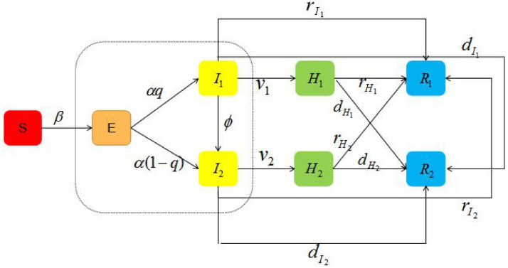
Here, we stratified the populations as susceptible (S), exposed (E), infectious with mild symptoms (I ₁), infectious with severe symptoms (I ₂), hospitalized patients with mild illness (H ₁), hospitalized patients with severe illness (H ₂), recovered (R ₁) and dead (R ₂). The incidence rate of exposed individual is α, and they became symptomatic after onset, which include patients with mild symptoms and severe symptoms, and the proportion of mild cases is q. Then, the exposed individuals, move to I ₁(I ₂) at a rate of $\alpha q\left(\alpha \right(1-q\left)\right)$. Mild cases will turn into severe cases in a certain proportion. Patients with severe symptoms will directly turn into recovered or dead after treatment, and those who will turn into mild cases is not considered. All severe patients are hospitalized and isolated, while those diagnosed in mild cases are hospitalized and isolated. The transformation relationship between persons with different epidemiological states is shown in Fig. 1 .

Fig. 1.

Transforming relationships between persons with different epidemiological states.

According to Fig. 1, the differential equation model is governed by the following system of equations:

$$\{\begin{array}{c}\dot{S}=-\beta ·S·\left(\eta ·E+I_1+I_2\right),\hfill \\ \dot{E}=\beta ·S·\left(\eta ·E+I_1+I_2\right)-\alpha ·E,\hfill \\ {\dot{I}}_1=\alpha ·q·E-\varphi ·I_1-v_1·I_1-r_{I_1}·I_1-d_{I_1}·I_1,\hfill \\ {\dot{I}}_2=\alpha ·\left(1-q\right)·E+\varphi ·I_1-v_2·I_2-r_{I_2}·I_2-d_{I_2}·I_2,\hfill \\ {\dot{H}}_1=v_1·I_1-r_{H_1}·H_1-d_{H_1}·H_1,\hfill \\ {\dot{H}}_2=v_2·I_2-r_{H_2}·H_2-d_{H_2}·H_2,\hfill \\ {\dot{R}}_1=r_{I_1}·I_1+r_{I_2}·I_2+r_{H_1}·H_1+r_{H_2}·H_2\hfill \\ {\dot{R}}_2=d_{I_1}·I_1+d_{I_2}·I_2+d_{H_1}·H_1+d_{H_2}·H_2.\hfill \end{array}$$ (1)

With the initial condition $S\left(0\right)={10}^7$, $E\left(0\right)=1$, $I_1\left(0\right)=0$, $I_2\left(0\right)=0$,$H_1\left(0\right)=0$, $H_2\left(0\right)=0$, $R_1\left(0\right)=0$, $R_2\left(0\right)=0$, this study was modeled in a population of 10,000,000 individuals, consistent with the size of Wuhan city [31]. In previous study, the infection rate of the susceptible to exposed is different from that of the infected, and the magnitude of it is 10^-8 [30]. Here, let the transmission probability β is 3 × 10^-8. The exposed individuals reduce infectivity with factor η(0 < η < 1) [30]. Previous study has shown that the median incubation period of all patients is 4 days [32], so the incidence rate of exposed individual$\alpha =1/4$. The implicit hypothesis in the model (1)is that the latent stage and the diseased stage are exponential distribution, and the total diseased stage is gamma distribution. Based on Health Commission of Hubei Province's report on COVID-19, the proportion of patients with mild symptoms is about 90% [33]. Considering the high admission rate of severe patients $\left(v_2=0.5\right)$, which is equivalent to the diagnosis within an average of two days after onset. In general, the time of diagnosis of patients with mild symptoms is longer than that of severe cases. Therefore, we take the hospital isolation rate of mild patients is no more than 0.5(v ₁ ≤ 0.5). The parameters in model (1)are shown in Table 1 .

Table 1.

The parameters in model (1).

Parameters	definitions	value	Unit
β	Probability of transmission	3 × 10-8[30]	Day−1
η	Decrease proportion of latent period infectivity	0.5 [30]	Dimensionless
α	Incidence rate of the exposed individual	0.25 [32]	Day−1
q	Proportion of patients with mild symptoms	0.9 [33]	Dimensionless
φ	proportion of mild cases that become severe	0.01	Dimensionless
v1	Hospital isolation rate of patients with mild symptoms	0–0.5	Day−1
v2	Hospital isolation rate of patients with severe symptoms	0.5	Day−1
$r_{I_1}$	Self - healing rate of patients with mild symptoms	0.05	Day−1
$r_{I_2}$	Self - healing rate of patients with severe symptoms	0.01	Day−1
$r_{H_1}$	Cure rate of hospitalized patients with mild symptoms	0.05	Day−1
$r_{H_2}$	Cure rate of hospitalized patientswith severe symptoms	0.04	Day−1
$d_{I_1}$	Death rate of patients with mild symptoms	0	Day−1
$d_{I_2}$	Death rate of patients with severe symptoms	0.04	Day−1
$d_{H_1}$	Death rate of hospitalized patients with mild illness	0	Day−1
$d_{H_2}$	Death rate of hospitalized patients with severe illness	0.01	Day−1

3. Results

3.1. Basic reproduction number

We use the next generation matrix [34] to calculate the basic reproduction number of model (1). There is a disease-free equilibrium point P ₀ when $S\left(0\right)=N$. The infected compartments are E, I ₁and I ₂. Note that $X={(E,I_1,I_2)}^T$, F(X) represents the matrix of new infectious diseases, V(X) represents the transfer matrix between the equations of infectious diseases. From model (1), it can be obtained that:

$$\begin{array}{ccc}\hfill F\left(X\right)& =& \left[\begin{array}{c}\beta ·S·(\eta ·E+I_1+I_2)\hfill \\ 0\hfill \\ 0\hfill \end{array}\right],\hfill \\ \hfill V\left(X\right)& =& \left[\begin{array}{c}\alpha ·E\hfill \\ -\alpha ·q·E+\phi ·I_1+v_1·I_1+r_{I_1}·I_1+d_{I_1}·I_1\hfill \\ -\alpha ·(1-q)·E-\phi ·I_1+v_2·I_2+r_{I_2}·I_2+d_{I_2}·I_2\hfill \end{array}\right],\hfill \end{array}$$

At the disease-free equilibrium point P ₀, the Jacobian matrices of F(X)and V(X) are respectively:

$$\begin{array}{ccc}\hfill F& =& \left[\begin{array}{ccc}\beta ·S_0·\eta \hfill & \beta ·S_0& \beta ·S_0\\ 0\hfill & 0& 0\\ 0\hfill & 0& 0\end{array}\right],\hfill \\ \hfill V& =& \left[\begin{array}{ccc}\alpha \hfill & 0& 0\\ -\alpha ·q\hfill & \phi +v_1+r_{I_1}+d_{I_1}& 0\\ -\alpha ·(1-q)\hfill & -\phi & v_2+r_{I_2}+d_{I_2}\end{array}\right],\hfill \end{array}$$

So the next generation matrix of model (1) is:

$$\begin{array}{c}\hfill F{V}^{-1}=\left[\begin{array}{ccc}\frac{\beta S_0\eta }{\alpha }+\frac{\beta S_{0}q}{\phi +v_1+r_{I_1}+d_{I_1}}-\frac{\beta S_0(d_{I_1}q+r_{I_1}q+v_{1}q-d_{I_1}-\phi -r_{I_1}-v_1)}{(\phi +v_1+r_{I_1}+d_{I_1})(v_2+r_{I_2}+d_{I_2})}\hfill & \frac{\beta S_0}{\phi +v_1+r_{I_1}+d_{I_1}}+\frac{\beta S_0\phi }{(\phi +v_1+r_{I_1}+d_{I_1})(v_2+r_{I_2}+d_{I_2})}& \frac{\beta S_0}{v_2+r_{I_2}+d_{I_2}}\\ 0\hfill & 0& 0\\ 0\hfill & 0& 0\end{array}\right].\end{array}$$

The maximum spectral radius of $F{V}^{-1}$is:

$$\begin{array}{c}\rho \left(F{V}^{-1}\right)=\frac{\beta S_0\eta }{\alpha }+\frac{\beta S_{0}q}{\phi +v_1+r_{I_1}+d_{I_1}}-\frac{\beta S_0(d_{I_1}q+r_{I_1}q+v_{1}q-d_{I_1}-\phi -r_{I_1}-v_1)}{(\phi +v_1+r_{I_1}+d_{I_1})(v_2+r_{I_2}+d_{I_2})}\hfill \\ =\beta S_0\left[\frac{\eta }{\alpha }+\frac{1}{{\mathrm{v}}_2+r_{I_2}+d_{I_2}}+\frac{q[(v_2-v_1)+(r_{I_2}-r_{I_1})+(d_{I_2}-d_{I_1})]}{(\phi +v_1+r_{I_1}+d_{I_1})({\mathrm{v}}_2+r_{I_2}+d_{I_2})}\right].\hfill \end{array}$$

Hence, the basic reproduction number of model(1) is:

$$R_0=\beta S_0\left[\frac{\eta }{\alpha }+\frac{1}{{\mathrm{v}}_2+r_{I_2}+d_{I_2}}+\frac{q[(v_2-v_1)+(r_{I_2}-r_{I_1})+(d_{I_2}-d_{I_1})]}{(\phi +v_1+r_{I_1}+d_{I_1})({\mathrm{v}}_2+r_{I_2}+d_{I_2})}\right].$$ (2)

3.2. numerical simulation

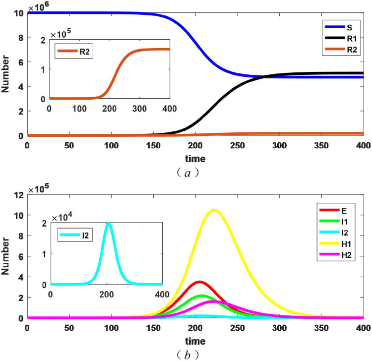
First of all, considering the isolation of patients with mild symptoms from the beginning of the outbreak. Supposing the hospital isolation rate of mild cases is 0.3($v_1=0.3$). The evolutionary results of persons with different epidemiological states are shown in Fig. 2 .

Fig. 2.

Changes in the number of persons with different epidemiological states with $v_1=0.3$.

From the Fig. 2 (a), the number of susceptible, dead, and recovered all tend to be stable. We say that the difference between the initial and the stble number of susceptible is the epidemic final size, so the epidemic final size tends to be stable. As can be obtained from the Fig. 2 (b), the number of exposed, patients with severe diseases, patients with mild diseases and hospitalized patients all have peaks. Among them, the peak value of hospitalized patients with mild symptoms is the highest, and the emergence time is the latest. The time when $E+I_1+I_2=0$is called the end of epidemic, and the corresponding value is the duration of the epidemic. The duration of the epidemic was 442 days with these parameters.

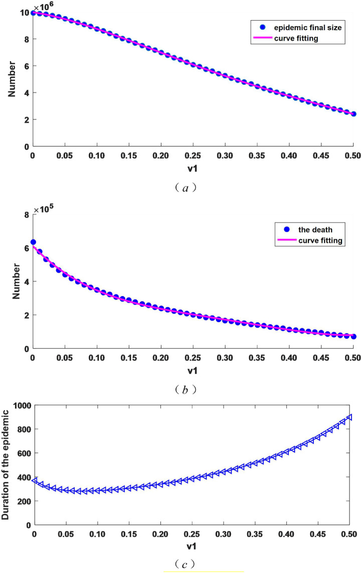
Secondly, we discuss the impact of different hospital isolation rates on the epidemic final size, the number of dead and duration of the outbreak. We take v ₁ in the range of 0 and 0.5 (v ₁ ∈ [0, 0.5], and $v_{1i}=0.01\times i,i=0,1\cdots 50$). Fig. 3 depicts the changes in the epidemic final size, the number of dead and duration of the epidemic.

Fig. 3.

When v₁ changes, the epidemic final size, the number of dead and the duration of the epidemic change.

As Fig. 3 (a) describes, with the increase of the isolation intensity v ₁, the final epidemic size become smaller and decrease by about 76%, from over 9.94 million when the patients with mild symptoms are not isolated ($v_1=0$) to over 2.42 million when the isolation intensity is 0.5. Therefore, increasing the isolation intensity for the mild cases can effectively reduce the epidemic final size. As can be seen from Fig. 3(b), similar to (a), the number of dead decreases, from more than 630,000 when the mild patients are not isolated ($v_1=0$) to more than 70,000 when the isolation intensity is 0.5, the reduction is about 89 percent. From Fig. 3(c), the duration of the epidemic becomes longer with the increase of the isolation intensity. Combined with (a) and (b), it can be seen that the epidemic extends with the decrease of the number of patients.

According to Eq. (2), we can obtain the basic reproduction number is 5.236326 or 1.145454 if isolation intensity of patients with mild symptoms is 0 or 0.5, so it reduced by about 78% compared with strong isolation intensity ($v_1=0.5$) and no measures for mild cases($v_1=0$). Therefore, increasing the hospitalized isolation rate for mild cases has a significant inhibitory effect on the transmission of COVID-19, which is consistent with the numerical simulation results in Fig. 3(a) and (b).

By data fitting, the analitical expressions of the curves in Fig. 3 (a) and (b) are obtained as follows:

$$\begin{array}{ccc}\hfill y_a& =& -1.34·{10}^8{v_1}^4+1.7105·{10}^8{v_1}^3-6.7876·{10}^7{v_1}^2\hfill \\ & & -7.247·{10}^6{v}_1+9.9873·{10}^6\hfill \end{array}$$ (3)

$$\begin{array}{ccc}\hfill y_b& =& 2.7502·{10}^7{v_1}^4-3.4447·{10}^7{v_1}^3-1.6083·{10}^7{v_1}^2\hfill \\ & & -3.9289·{10}^6{v}_1+6.0992·{10}^5\hfill \end{array}$$ (4)

We can get the epidemic final size and the number of dead for a given isolation measure using these two expressions(3) and (4), which gives us a better understanding of the epidemic.

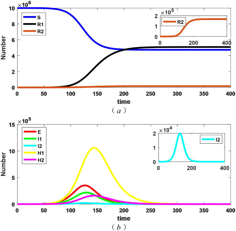
In addition, we consider that patients with mild symptoms are not isolated in the first place. Supposing that the time of starting to adopt isolation measures for mild cases is t ₁. When t is less than t ₁(t < t ₁), the hospital isolation rate of mild patients is 0, and when t is greater than t ₁ (t ≥ t ₁), the hospital isolation rate is 0.3 ($v_1=0.3$). Here, Fig. 4 presents the evolution results of persons with different epidemiological states with $v_1=0.3$, $t_1=50$.

Fig. 4.

Changes in the number of people of persons with different epidemiological states when $t_1=50$.

By the Fig. 4, the number of susceptible, dead, and recovered all tend to be stable, and thus the epidemic final size also tends to be stable. There are peaks in exposed, unquarantined patients and hospital patients, which are the same as the nature of Fig. 2, but the specific values are different. Here, the corresponding results at $t_1=50$and other values of t ₁ are taken, how do they correspond to the epidemic final size, the number of dead and the duration of the epidemic, which is discussed below.

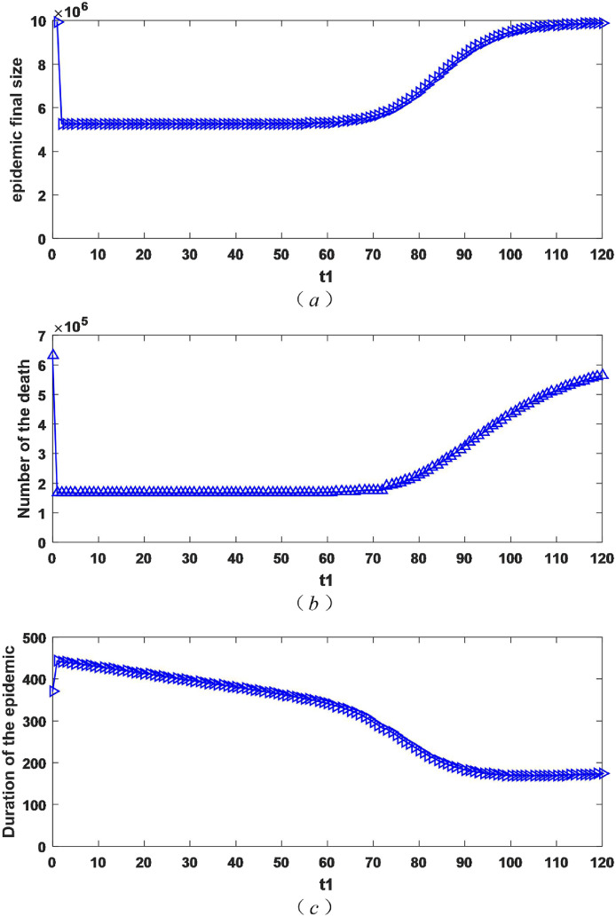
Considering the isolation rate of patients with mild symptoms may change vary from moment to moment, we take t ₁ within the scope of 0 and 120 (t ₁ ∈ [0, 120]). The value of hospital isolation rate is the same as that mentioned above($t<t_1,v_1=0;t\ge t_1,v_1=0.3$).The change of the epidemic final size, the number of dead and the duration of the epidemic as shown in Fig. 5 .

Fig. 5.

The impact of different starting moment of mild isolation measures on the epidemic final size, the number of dead and the duration of epidemic.

As obtained in Fig. 5 (a), as the time to start isolation measures is delayed, the final size of epidemic gets larger. It's worth noting that there is a time t ₀. When t ₁ is less than t ₀ (t ₁ < t ₀), if the measure is started one day later, the increase in the epidemic final size is not large. However, when t ₁ is higher than t ₀(t ₁ > t ₀), if the measure is taken one day later, the epidemic final size may increases a lot. At this point, it is obvious to adopt measures early. Fig. 5 (b) describes the number of dead increases with the delay in the initiation of isolation measures. Similar to (a), there is a moment t ₀ (same as (a)). When t ₁ is less than t ₀ (t ₁ < t ₀), start taking measures one day later, the increment of the number of dead is not large, but when t ₁ is higher than t ₀(t ₁ > t ₀), the number of dead has increased dramatically. From Fig. 5 (c), the duration of the epidemic is shortened with the delay in the initiation of isolation measures for patients with mild illness. Combined with (a) and (b), it can be seen that this is the result of the aggravation of the epidemic.

As can be seen from Fig. 5, the earlier the isolation measures for patients with mild symptoms are, the better the effect will be. Taking into account that measures are adopted one day later may bring serious consequences, the isolation measures for mild cases should be adopted in time as long as possible.

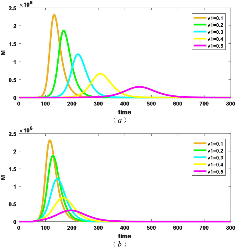
Finally, we discuss the number of beds required for different measures in the two different situations where isolation measures are taken for patients with mild illness from the beginning and after 50 days. If M is the required number of total beds, then $M\left(t\right)=H_1\left(t\right)+H_2\left(t\right)$. Fig. 6 shows the number of beds required for different isolation intensities ($v_1=0.1,0.2,0.3,0.4,0.5$) over time.

Fig. 6.

Changes in the number of beds required for different isolation measures . (a) taking isolation measures from the beginning; (b) taking isolation measures after 50 days.

As can be seen from Fig. 6 (a), when patients with mild illness are quarantined from the outset, the greater the intensity of isolation, the smaller the peak of the number of beds required, and the time to reach the peak is delayed, which is the result of the decrease in the final size of epidemic as the intensity of isolation increases. As can be obtained in Fig. 6 (b), when isolation measures are taken from 50 days($t\le 50,v_1=0;t>50,v_1>0$), similar to figure (a), the greater the intensity of isolation measures, the smaller the peak of the required number of beds, and the time to reach the peak will be delayed. By comparing (a) and (b), it can be seen that for the same level of isolation, measures taken after 50 days will peak earlier than those taken from the outset, and the greater v ₁is, the more obvious the time difference is. Table 2 shows the maximum number of beds required for different isolation measures and the moment when the maximum value is reached in Fig. 6.

Table 2.

The maximum number of beds required for different isolation measures and the moment when the maximum value is reached in Fig. 6.

	$t_1=0$		$t_1=50$
	Mmax	tmax	Mmax	tmax
$v_1=0.1$	2,309,341	132	2,310,583	117
$v_1=0.2$	1,867,075	168	1,872,214	128
$v_1=0.3$	1,208,139	222	1,218,071	145
$v_1=0.4$	664,956	306	680,275	167
$v_1=0.5$	295,619	454	316,347	195

As can be seen from Table 2, the earlier isolation measures are taken, the smaller the peak of the number of beds required, but the reduction is modest. By comparing the moments that reached the maximum in the Table 2, we can find that the late adoption of measures makes the time to reach the maximum significantly earlier, that is to say, which makes the maximum number of hospital beds appear in advance, and is not conducive to the allocation of emergency beds. Therefore, early isolation measures for patients with mild illness can make the pressure of medical resource demand appear later. For example, the effectiveness of such missions as Huoshenshan, Leishenshan, and Fangcang hospitals is based on the premise that the maximum number of patients appears later.

4. Conclusion

In the course of COVID-19 epidemic development, due to the neglect of patients with mild disease, the isolation measures for them are relatively weak, and some are not even adopted, but mild patients are also capable of infection. The hospital isolation measures for mild cases can quickly and strictly control the source of infection and prevent the spread of the virus in the community and family. In addition, through the medical means, the vast majority of mild patients not only can be significantly improved, but also achieve the effect of rehabilitation. What's more, the rate of patients from mild to severe is reduced.

In this paper, we study the effect of isolation measures on the epidemic fianl size, the number of dead and duration of the epidemic. The results show that isolation measures can significantly reduce the epidemic final size and the number dead, and the greater the intensity of measures, the better, but duration of the epidemic will be prolonged. In early stage of the epidemic, taking measures one day later has little impact, but after a certain period, if taking measures one day later, the epidemic final size and the number of dead increase sharply. Taking measures as early as possible makes the maximum number of patients appear later, which is conducive to expanding medical bed resources and reducing the pressure on medical resource demand. As long as possible, high-intensity isolation measures should be taken in time for patients with mild symptoms.

In this paper, the hospital isolation measures for patients with mild illness do not change over time, and it is reasonable to change over time, which can be continued to work.

Declaration of Competing Interest

The authors declare that they have no known competing financial interests or personal relationships that could have appeared to influence the work reported in this paper.

References

- 1.Ambat A.S., Vyas N. Assessment of preparedness against emerging infectious disease amongprivate hospitals in a district of South India. Med J Armed Forces India. 2020 doi: 10.1016/j.mjafi.2020.02.007. [DOI] [PMC free article] [PubMed] [Google Scholar]
- 2.Cupertino M.C., et al. Emerging and re-emerging human infectious diseases: a systematic review of the role of wild animals with a focus on public health impact. Asian Pac J Trop Med. 2020;13(3):99–106. [Google Scholar]
- 3.Lam S.K.K., et al. Investigating the Strategies Adopted by Emergency Nurses to Address Uncertainty and Change in the Event of Emerging Infectious Diseases: a Grounded Theory Study. Int J Environ Res Public Health. 2020;17(7) doi: 10.3390/ijerph17072490. [DOI] [PMC free article] [PubMed] [Google Scholar]
- 4.Rachowicz L.J., et al. The novel and endemic pathogen hypotheses: competing explanations for the origin of emerging infectious diseases of wildlife. Conservation Biology. 2005;19(5):1441–1448. [Google Scholar]
- 5.Wu Z., et al. Comparative analysis of rodent and small mammal viromes to better understand the wildlife origin of emerging infectious diseases. Microbiome. 2018;6 doi: 10.1186/s40168-018-0554-9. [DOI] [PMC free article] [PubMed] [Google Scholar]
- 6.Wu Z., et al. Deciphering the bat virome catalog to better understand the ecological diversity of bat viruses and the bat origin of emerging infectious diseases. Isme Journal. 2016;10(3):609–620. doi: 10.1038/ismej.2015.138. [DOI] [PMC free article] [PubMed] [Google Scholar]
- 7.McBryde E. The value of early transmission dynamic studies in emerging infectious diseases. Lancet Infect Dis. 2020 doi: 10.1016/S1473-3099(20)30161-4. [DOI] [PMC free article] [PubMed] [Google Scholar]
- 8.Oei W., et al. Modeling the transmission risk of emerging infectious diseases through blood transfusion. Transfusion. 2013;53(7):1421–1428. doi: 10.1111/j.1537-2995.2012.03941.x. [DOI] [PubMed] [Google Scholar]
- 9.Wendelboe A.M., Grafe C., Carabin H. The Benefits of Transmission Dynamics Models in Understanding Emerging Infectious Diseases. American Journal Of the Medical Sciences. 2010;340(3):181–186. doi: 10.1097/MAJ.0b013e3181e937ca. [DOI] [PMC free article] [PubMed] [Google Scholar]
- 10.Li G., Dong Y. Dynamic modelling of the impact of public health education on the control of emerging infectious disease. J Biol Dyn. 2019;13(1):502–517. doi: 10.1080/17513758.2019.1639835. [DOI] [PubMed] [Google Scholar]
- 11.Brug J., Aro A.R., Richardus J.H., Risk Perceptions, Behaviour Towards Pandemic Control of Emerging Infectious Diseases International Research on Risk Perception in the Control of Emerging Infectious Diseases. Int J Behav Med. 2009;16(1):3–6. doi: 10.1007/s12529-008-9000-x. [DOI] [PMC free article] [PubMed] [Google Scholar]
- 12.Maki D.G., revisited S.A.R.S. The challenge of controlling emerging infectious diseases at the local, regional, federal, and global levels. Mayo Clin. Proc. 2004;79(11):1359–1366. doi: 10.4065/79.11.1359. [DOI] [PMC free article] [PubMed] [Google Scholar]
- 13.Krause R.M., Dimmock N.J., Morens D.M. Summary of antibody workshop: the role of humoral immunity in the treatment and prevention of emerging and extant infectious diseases. Journal Of Infectious Diseases. 1997;176(3):549–559. doi: 10.1086/514074. [DOI] [PubMed] [Google Scholar]
- 14.Kumar S., et al. Recent Advances in Vaccine Development for the Treatment of Emerging Infectious Diseases. Indian Journal Of Pharmaceutical Education And Research. 2019;53(3):343–354. [Google Scholar]
- 15.Jones K.E., et al. Global trends in emerging infectious diseases. Nature. 2008;451(7181) doi: 10.1038/nature06536. 990-U4. [DOI] [PMC free article] [PubMed] [Google Scholar]
- 16.Gomez J.M., Nunn C.L., Verdu M. Proceedings Of the National Academy Of Sciences Of the United States Of America. Vol. 110. 2013. Centrality in primate-parasite networks reveals the potential for the transmission of emerging infectious diseases to humans; pp. 7738–7741. [DOI] [PMC free article] [PubMed] [Google Scholar]
- 17.Chen S., et al. Fangcang shelter hospitals: a novel concept for responding to public health emergencies. The Lancet. 2020 doi: 10.1016/S0140-6736(20)30744-3. [DOI] [PMC free article] [PubMed] [Google Scholar]
- 18.Fang Y., Nie Y., Penny M. Transmission dynamics of the COVID-19 outbreak and effectiveness of government interventions: a data-driven analysis. J. Med. Virol. 2020;92(6):645–659. doi: 10.1002/jmv.25750. [DOI] [PMC free article] [PubMed] [Google Scholar]
- 19.Roberts M.G., Nishiura H. Early Estimation of the Reproduction Number in the Presence of Imported Cases: pandemic Influenza H1N1-2009 in New Zealand. PLoS ONE. 2011;6(5) doi: 10.1371/journal.pone.0017835. [DOI] [PMC free article] [PubMed] [Google Scholar]
- 20.Wallinga J., Teunis P. Different epidemic curves for severe acute respiratory syndrome reveal similar impacts of control measures. Am. J. Epidemiol. 2004;160(6):509–516. doi: 10.1093/aje/kwh255. [DOI] [PMC free article] [PubMed] [Google Scholar]
- 21.Fisman D., Khoo E., Tuite A. Early epidemic dynamics of the west african 2014 ebola outbreak: estimates derived with a simple two-parameter model. PLoS Curr. 2014;6 doi: 10.1371/currents.outbreaks.89c0d3783f36958d96ebbae97348d571. [DOI] [PMC free article] [PubMed] [Google Scholar]
- 22.Wu J.T., Leung K., Leung G.M. Nowcasting and forecasting the potential domestic and international spread of the 2019-nCoV outbreak originating in Wuhan. China: a modelling study. Lancet. 2020;395(10225):689–697. doi: 10.1016/S0140-6736(20)30260-9. [DOI] [PMC free article] [PubMed] [Google Scholar]
- 23.Tang B., et al. An updated estimation of the risk of transmission of the novel coronavirus (2019-nCov) Infectious Disease Modelling. 2020;5:248–255. doi: 10.1016/j.idm.2020.02.001. [DOI] [PMC free article] [PubMed] [Google Scholar]
- 24.Tang B., et al. Estimation of the Transmission Risk of the 2019-nCoV and Its Implication for Public Health Interventions. J Clin Med. 2020;9(2) doi: 10.3390/jcm9020462. [DOI] [PMC free article] [PubMed] [Google Scholar]
- 25.Greenhalgh D. Some results for an SEIR epidemic model with density dependence in the death rate. IMA J Math Appl Med Biol. 1992;9(2):67–106. doi: 10.1093/imammb/9.2.67. [DOI] [PubMed] [Google Scholar]
- 26.Li M.Y., Muldowney J.S. Global stability for the SEIR model in epidemiology. Math Biosci. 1995;125(2):155–164. doi: 10.1016/0025-5564(95)92756-5. [DOI] [PubMed] [Google Scholar]
- 27.Deguen S., Thomas G., Chau N.P. Estimation of the contact rate in a seasonal SEIR model: application to chickenpox incidence in France. Stat Med. 2000;19(9):1207–1216. doi: 10.1002/(sici)1097-0258(20000515)19:9<1207::aid-sim423>3.0.co;2-l. [DOI] [PubMed] [Google Scholar]
- 28.Li M.Y., et al. Global dynamics of a SEIR model with varying total population size. Math Biosci. 1999;160(2):191–213. doi: 10.1016/s0025-5564(99)00030-9. [DOI] [PubMed] [Google Scholar]
- 29.Gumel A.B., et al. Modelling strategies for controlling SARS outbreaks. Proceedings Of the Royal Society B-Biological Sciences. 2004;271(1554):2223–2232. doi: 10.1098/rspb.2004.2800. [DOI] [PMC free article] [PubMed] [Google Scholar]
- 30.Yang Z., et al. Modified SEIR and AI prediction of the epidemics trend of COVID-19 in China under public health interventions. J Thorac Dis. 2020;12(3) doi: 10.21037/jtd.2020.02.64. 165-+ [DOI] [PMC free article] [PubMed] [Google Scholar]
- 31.Maugeri A., et al. Estimation of Unreported Novel Coronavirus (SARS-CoV-2) Infections from Reported Deaths: a Susceptible-Exposed-Infectious-Recovered-Dead Model. J Clin Med. 2020;9(5) doi: 10.3390/jcm9051350. [DOI] [PMC free article] [PubMed] [Google Scholar]
- 32.Guan W., et al. Clinical Characteristics of Coronavirus Disease 2019 in China. New England Journal Of Medicine. 2020;382(18):1708–1720. doi: 10.1056/NEJMoa2002032. [DOI] [PMC free article] [PubMed] [Google Scholar]
- 33.Health Commission of Hubei Province. http://wjw.hubei.gov.cn/bmdt/ztzl/fkxxgzbdgrfyyq/. Accessed 29 February 2020.
- 34.van den Driessche P., Watmough J. Reproduction numbers and sub-threshold endemic equilibria for compartmental models of disease transmission. Math Biosci. 2002;180:29–48. doi: 10.1016/s0025-5564(02)00108-6. [DOI] [PubMed] [Google Scholar]