Optimal Control Design of Impulsive SQEIAR Epidemic Models with Application to COVID-19

Abstract

This paper presents a SEIAR-type model considering quarantined individuals (Q), called SQEIAR model. The dynamic of SQEIAR model is defined by six ordinary differential equations that describe the numbers of Susceptible, Quarantined, Exposed, Infected, Asymptomatic, and Recovered individuals. The goal of this paper is to reduce the size of susceptible, infected, exposed and asymptomatic groups to consequently eradicate the infection by using two actions: the quarantine and the treatment of infected people. To reach this purpose, optimal control theory is presented to control the epidemic model over free terminal optimal time control with an optimal cost. Pontryagin's maximum principle is used to characterize the optimal controls and the optimal final time. Also, an impulsive epidemic model of SQEIAR is considered to deal with the potential suddenly increased in population caused by immigration or travel. Since this model is suitable to describe the COVID-19 pandemic, especial attention is devoted to this case. Thus, numerical simulations are given to prove the accuracy of the theoretical claims and applied to the particular data of this infection. Moreover, numerical computations of the COVID-19 are compared with diseases like Ebola and Influenza. In addition, the controller is evaluated with system parameters identified by using actual data of China. Finally, the controller tuned with the estimated parameters of the Chinese data is applied to the actual data of Spain to compare the quarantine and treatment policies in both countries.

Introduction

Coronaviruses are a group of viruses that cause infection ranging from a usual cold to Severe Acute Respiratory Syndrome (SARS) [1]. According to the World Health Organization, the current coronavirus disease (COVID-19) was first reported in Wuhan, China, on 31 December 2019. General symptoms of this infection are respiratory symptoms such as cough, fever, breathing problems, and shortness of breath. In more critical cases, pneumonia, kidney failure, severe acute respiratory syndrome, and even death have also been reported [2]. Given that COVID-19 is an unknown disease, it is understandable that its development and spread cause nervousness and fear. As a result, we decided to represent a more complete model than the other works used, [1], and control the infection with an optimal control strategy. According to [3], that presents a new (SEIAR) model for influenza, in the present paper we introduce a related and also new model with a difference. Since the coronavirus (or any similar infection) does not have a vaccine yet, in our new model, in addition to Susceptible, Exposed, Infected, Asymptomatic, and Recovered individuals (SEIAR), we added a new group of people called “people in quarantine”. In addition to continuous-time systems, system dynamics can also be described by discrete-time SEIR epidemic models [4, 5]. To furthermore study about discrete-time SEIR epidemic models with time delay, readers are referred to [6].

It is obvious that transportation among regions has also a strong impact on the dynamic evolution of a disease which can spread the infection on a large scale. Thus, [7] considers an SEIR epidemic model and investigated the impact of transport-related infection between two cities. Generally, the number of the population may grow because of travel or immigration during a period. Therefore, impulsive change of population should be considered, which is generates an impulsive epidemic model. The phenomena of ‘impulsive epidemic model’ has important biological meaning in epidemic models. Impulse is included in epidemic disease models, which greatly improves biological background [8]. There are some studies examining this subject including [9] where a system of impulsive functional differential equations is studied by using new computational techniques for impulsive differential equations and [10], that investigated the stability of impulsive delayed nonlinear hybrid differential systems. Accordingly, in this paper, we consider a number of susceptible, infected, asymptomatic and exposed individuals as an impulsive additive population to the community on a daily basis, which describe the fact that the coronavirus is spread by the travel of people unaware of the disease that is added to the population impulsively. Among these models which have used impulsive strategy, impulsive control has attracted many interests, which in this article can be seen as an example of this impulsive control [11], [12], [13], [14]. Optimal control methods are used to control numerous kinds of models especially dynamic epidemic models [15], [16], [17], [18], [19], [20]. The adaptability and relative simplicity of optimal control methods can lead to the improvement of the strategies to control the different kinds of diseases [21, 22]. Human mobility is a critical issue in epidemic models. Thus, for studying the transmission of infectious diseases and improving epidemic control we also can use the large-scale systems. We refer to [23] that deals with the application of optimal control in large-scale systems that can also be used in epidemic systems. Therefore, in this paper, the optimal control strategy is applied to the SQEIAR model to decrease the number of susceptible, infected, exposed and asymptomatic individuals in the optimal time. It has been proved that as a result of this that the number of people in quarantine and the total population is increased. China, where the virus first began to spread in late 2019, has seen an obvious reduction in its rate of new cases and people known to be infected have since recovered, this is only for strict quarantine and treatment of infected people. Also, Spain is another country hit by COVID-19. Therefore, in this study, the accuracy of the controller designed on the estimated parameters using real data of China has also been examined and the process of controlling COVID-19 in both countries will be investigated. Accordingly, in this paper, it was decided to compare the results of the study with the actual data to evaluate the performance of this controller.

The rest of this paper is divided into 7 sections: In the first section, we introduce and explain the SEIAR model in detail, after that the optimal control strategy is applied to the SQEIAR dynamic model in Section 2. Also, an impulsive SQEIAR epidemic model is introduced in Section 3. In Section 4 the proposed controller applied to impulsive SQEIAR epidemic model. In the following and in the fifth section, the results of simulations under different cases are presented. The comparison of the results of this study with other diseases and actual data is mentioned in section 6. Finally, in section 7 the article ends with conclusions.

1. SEIAR Epidemic Model

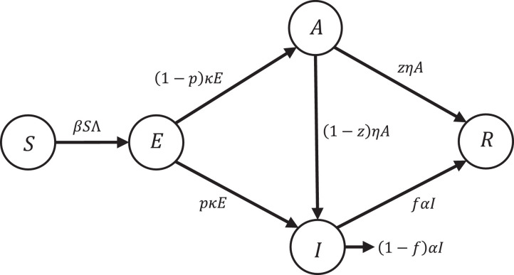
In this section, we explain the SEIAR epidemic model taken from [3] but we skipped births and natural mortality (because of the low μ rate in [3]). This assumption is feasible since the total population does not change significantly during the spreading time and we aim at controlling the disease as quickly as possible. The nonlinear SEIAR epidemiological model includes five non-negative state variables S(t), E(t), I(t), A(t) and R(t) that are defined as Susceptible, Exposed, Infected, Asymptomatic, and Recovered people, respectively. Here, S(t) represents the number of individuals who are susceptible to the infection (i.e. they are not infected yet). When a susceptible individual gets infected (i.e. becomes exposed to the infection, they move to the exposed people group (E(t)) that denotes the number of individuals who are exposed to infection (they are infected but they cannot transmit the virus). Finally, they reach a level that can transmit the disease at the rate of κ but a fraction of them have symptoms and the other fraction does not have any visible symptoms. We call them infected and asymptomatic and they are denoted by I(t) and A(t), respectively. The fraction p of exposed people moves to the infected people group and can transmit the infection to the others and the fraction $\left(1-p\right)$ of them goes to the asymptomatic people group who are infected with no symptoms of infection (A(t)). The fraction f of infected people become recovered at the rate of α and the remaining of them (the fraction $\left(1-f\right)$) will die because of the infection. Therefore, R(t) denotes the recovered people from the virus, and finally, N(t) is the total population size. Fig. 1 shows a flow diagram of SEIAR dynamic model. The dynamic model is mathematically described as:

$$\dot{S}\left(t\right)=-\beta \Lambda \left(\mathrm{t}\right)S\left(t\right)$$ (1-a)

$$\dot{E}\left(t\right)=\beta \Lambda \left(\mathrm{t}\right)S\left(t\right)-\kappa E\left(t\right)$$ (1-b)

$$\dot{I}\left(t\right)=\left(1-z\right)\eta A\left(t\right)-\alpha I\left(t\right)+p\kappa E\left(t\right)$$ (1-c)

$$\dot{A}\left(t\right)=\left(1-p\right)\kappa E\left(t\right)-\eta A\left(t\right)$$ (1-d)

$$\dot{R}\left(t\right)=z\eta \mathrm{A}\left(t\right)+f\alpha I\left(t\right)$$ (1-e)

here, $N\left(t\right)=S\left(t\right)+E\left(t\right)+I\left(t\right)+A\left(t\right)+R\left(t\right)$, $\Lambda \left(\mathrm{t}\right)=\epsilon E\left(t\right)+\left(1-q\right)I\left(t\right)+\delta A\left(t\right)$. The non-negative initial conditions are $(S\left(0\right),E\left(0\right),I\left(0\right),A\left(0\right),R\left(0\right))=\left(S_0,E_0,I_0,A_0,R_0\right)$. The state variables and parameters are positive values. For further study, view [3, 24].

Fig. 1.

Conceptual flow diagram of the SEIAR dynamic epidemic model.

2. The Optimal Control Problem of SQEIAR Epidemic Model

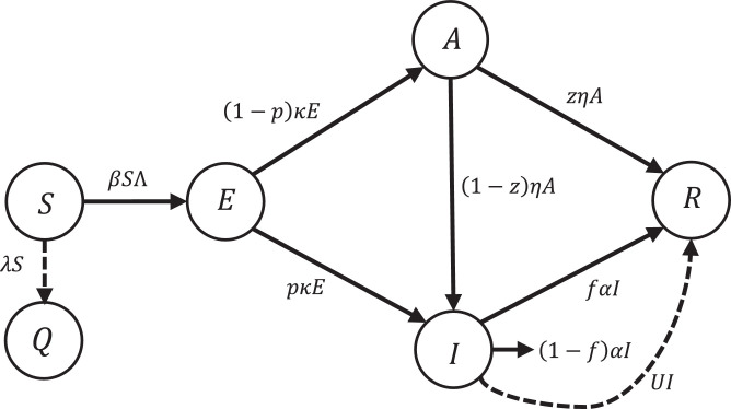
Since the vaccines that we have against the virus do not work and recovery depends on the strength of the immune system, many of those who have died were already in poor health. So, at the moment, the best way to prevent the spread of the virus is to quarantine susceptible people against the infection. Therefore, in this section, we want to use optimal control theory to eradicate the epidemic within the shortest pre-defined period of time (for example 10 days) by quarantining susceptible people and by applying antiviral therapies to infected people. A number of susceptible people must become quarantined at the rate of λ(t), that means they move to a group called quarantined people, described by Q(t). After eradication of the disease the total size of people almost includes the quarantined and recovered people$\left(R\left(t\right)+Q\left(t\right)\cong N\left(t\right)\right),$because a percentage of infected people will die because of infection and not all of them recover. Fig. 2 shows the flow diagram of SQEIAR dynamic model in the presence of the controller (i.e. the addition of the extra state Q(t) is indeed a control action on the SEAIR model describing the spread of the infection). The dynamic model with the controller is given by:

$$\dot{S}\left(t\right)=-\left(\beta \Lambda \left(\mathrm{t}\right)+\lambda \left(t\right)\right)S\left(t\right)$$ (2-a)

$$\dot{Q}\left(t\right)=\lambda \left(t\right)S\left(t\right)$$ (2-b)

$$\dot{E}\left(t\right)=\beta \Lambda \left(\mathrm{t}\right)S\left(t\right)-\kappa E\left(t\right)$$ (2-c)

$$\dot{I}\left(t\right)=\left(1-z\right)\eta A\left(t\right)-\alpha I\left(t\right)+p\kappa E\left(t\right)-U\left(t\right)I\left(t\right)$$ (2-d)

$$\dot{A}\left(t\right)=\left(1-p\right)\kappa E\left(t\right)-\eta A\left(t\right)$$ (2-e)

$$\dot{R}\left(t\right)=z\eta \mathrm{A}\left(t\right)+f\alpha I\left(t\right)+U\left(t\right)I\left(t\right)$$ (2-f)

where,$N\left(t\right)=S\left(t\right)+Q\left(t\right)+E\left(t\right)+I\left(t\right)+A\left(t\right)+R\left(t\right)$.

Fig. 2.

Conceptual flow diagram of the SQEIAR dynamic model with the proposed controller.

In optimal control theory, the main objective is the minimization of the number of the susceptible, infected, exposed and asymptomatic population while minimizing the cost of applying the controls U(t) (0 ≤ U(t) ≤ 1, treatment), and controls λ(t) (0 ≤ λ(t) ≤ 1, quarantine) in an optimal time interval. Therefore, the problem is to minimize the cost function J with a free terminal optimal time control:

$$\begin{array}{ccc}& & J\left(U\left(t\right),\lambda \left(t\right),T\right)\hfill \\ & & =\underset{0}{\overset{T}{\int }}\left[A_{1}I\left(t\right)+A_{2}A\left(t\right)+A_{3}E\left(t\right)+A_{4}S\left(t\right)+\frac{A_5}{2}U{\left(t\right)}^2+\frac{A_6}{2}\lambda {\left(t\right)}^2\right]\hfill \\ & & dt+\varnothing \left(T\right)\hfill \end{array}$$ (3)

A₁, A₂, A₃, and A₄ are the gains of the infected, asymptomatic, exposed, and susceptible individuals, respectively. Also, A ₅ and A ₆ are the gains of controllers with final fixed pre-defined time T. ∅(t) is a positive increasing function such that $\underset{t\to \infty }{lim}\varnothing \left(t\right)=\infty$. In other words, we want to reach the optimal controls (U*(t), λ*(t)) in an optimal terminal time (T*) such that $J\left(U^{*}\left(t\right),T^{*}\right)=min\left\{J\left(U\left(t\right),T\right)|U\left(t\right)\in U_1,T\in {\mathbb{R}}^{+}\right\}$ and $J\left({\lambda }^{*}\left(t\right),T^{*}\right)=min\left\{J\left(\lambda \left(t\right),T\right)|\lambda \left(t\right)\in U_2,T\in {\mathbb{R}}^{+}\right\}.$ The set of admissible controls defined by U ₁ and U ₂ as $U_1=\{U\left(t\right)\left|U\right(t)$ is measurable, $0\le U\left(t\right)\le U_{max}=1,t\in \left[0,T\right]\}$and similarly $U_2=\{\lambda \left(t\right)\left|\lambda \right(t)$ is measurable, $0\le \lambda \left(t\right)\le {\lambda }_{max}=1,t\in \left[0,T\right]\}$. The necessary conditions for optimality are expressed by:

$$\begin{array}{ccc}& & {\left[{\nabla }_{x_f}^{\varnothing }-p\left(t_f\right)\right]}^T\delta x_f\hfill \\ & & +\left[H\left(x\left(t_f\right),U\left(t_f\right),\lambda \left(t_f\right),p\left(t_f\right),t_f\right)+\frac{\partial \varnothing }{\partial t_f}\right]\delta t_f=0\hfill \end{array}$$ (4)

Here, the gradient $\left({\nabla }_{x_f}^{\varnothing }\right)$ is the derivative of ∅(x_f, t_f) with respect to x_f, and t_f is final time. Since x(t_f) is constant value (The final value of all states is known) then $\delta x_f=0$ and H is Hamiltonian, given as:

$$H=g+p^T\left(t\right)f$$ (5)

where, $p\left(t\right)=\left[p_1\left(t\right),p_2\left(t\right),p_3\left(t\right),p_4\left(t\right),p_5\left(t\right),p_6\left(t\right)\right]$ such that p ₁(t), p ₂(t), p ₃(t), p ₄(t), p ₅(t), and p ₆(t) are adjoint variables and $g=\left[A_{1}I\left(t\right)+A_{2}A\left(t\right)+A_{3}E\left(t\right)+A_{4}S\left(t\right)+\frac{A_5}{2}U{\left(t\right)}^2+\frac{A_6}{2}\lambda {\left(t\right)}^2\right]$ and $f=\dot{x}={\left[\dot{S}\left(t\right),\dot{Q}\left(t\right),\dot{E}\left(t\right),\dot{I}\left(t\right),\dot{A}\left(t\right),\dot{R}\left(t\right)\right]}^T$. Therefore, in this study the Hamiltonian yields as:

$$H=A_{1}I\left(t\right)+A_{2}A\left(t\right)+A_{3}E\left(t\right)+A_{4}S\left(t\right)+\frac{A_5}{2}U{\left(t\right)}^2+\frac{A_6}{2}\lambda {\left(t\right)}^2+p_1\left(t\right)\dot{S}\left(t\right)+p_2\left(t\right)\dot{Q}\left(t\right)+p_3\left(t\right)\dot{E}\left(t\right)+p_4\left(t\right)\dot{I}\left(t\right)+p_5\left(t\right)\dot{A}\left(t\right)+p_6\left(t\right)\dot{R}\left(t\right)$$ (6)

also,

$$\dot{p}\left(t\right)=-\frac{\partial H}{\partial x\left(t\right)}={\left[-\frac{\partial H}{\partial S\left(t\right)},-\frac{\partial H}{\partial Q\left(t\right)},-\frac{\partial H}{\partial E\left(t\right)},-\frac{\partial H}{\partial I\left(t\right)},-\frac{\partial H}{\partial A\left(t\right)},-\frac{\partial H}{\partial R\left(t\right)}\right]}^T$$ (7)

To calculate the necessary conditions, we use Pontryagin's maximum principle as follows:

Theorem

Given optimal controls (U*(t), λ*(t)) and solutions S*(t), Q*(t), E*(t), I*(t), A*(t), and R*(t) of the corresponding system, there exists adjoint variables p ₁(t), p ₂(t), p ₃(t), p ₄(t), p ₅(t), and p ₆(t) that satisfy

$${\dot{p}}_1\left(t\right)=-\frac{\partial H}{\partial S\left(t\right)}=-A_4+\lambda \left(t\right)\left[p_1\left(t\right)-p_2\left(t\right)\right]+\left(\beta \left(1-q\right)I\left(t\right)+\beta \epsilon E\left(t\right)+\beta \delta A\left(t\right)\right)\left[p_1\left(t\right)-p_3\left(t\right)\right]$$ (8-a)

$${\dot{p}}_2\left(t\right)=-\frac{\partial H}{\partial Q\left(t\right)}=0$$ (8-b)

$${\dot{p}}_3\left(t\right)=-\frac{\partial H}{\partial E\left(t\right)}=-A_3+\beta \epsilon S\left(t\right)\left[p_1\left(t\right)-p_3\left(t\right)\right]+\kappa \left[p_3\left(t\right)-p_5\left(t\right)\right]+p\kappa \left[p_5\left(t\right)-p_4\left(t\right)\right]$$ (8-c)

$${\dot{p}}_4\left(t\right)=-\frac{\partial H}{\partial I\left(t\right)}=-A_1+\beta \left(1-q\right)S\left(t\right)\left[p_1\left(t\right)-p_3\left(t\right)\right]+U\left(t\right)\left[p_4\left(t\right)-p_6\left(t\right)\right]+\alpha \left[p_4\left(t\right)-p_6\left(t\right)f\right]$$ (8-d)

$${\dot{p}}_5\left(t\right)=-\frac{\partial H}{\partial A\left(t\right)}=-A_2+\eta \left[p_5\left(t\right)-p_4\left(t\right)\right]+z\eta \left[p_4\left(t\right)-p_6\left(t\right)\right]+\beta \delta S\left(t\right)\left[p_1\left(t\right)-p_3\left(t\right)\right]$$ (8-e)

$${\dot{p}}_6\left(t\right)=-\frac{\partial H}{\partial R\left(t\right)}=0$$ (8-f)

where, $p_i\left(T\right)=0,i=1,\dots ,6$. By using the optimality conditions, we can solve the optimal controls as ${\nabla }_{U\left(t\right)}^H=0$ and ${\nabla }_{\lambda \left(t\right)}^H=0$. Therefore:

$$U^{*}\left(t\right)=\frac{I^{*}\left(t\right)\left[p_4\left(t\right)-p_6\left(t\right)\right]}{A_5}$$ (9)

and

$${\lambda }^{*}\left(t\right)=\frac{S^{*}\left(t\right)\left[p_1\left(t\right)-p_2\left(t\right)\right]}{A_6}$$ (10)

therefore,

$$U^{*}\left(t\right)=\{\begin{array}{cc}1& \frac{I^{*}\left(t\right)\left[p_4\left(t\right)-p_6\left(t\right)\right]}{A_5}\ge 1\\ \frac{I^{*}\left(t\right)\left[p_4\left(t\right)-p_6\left(t\right)\right]}{A_5}& 0<\frac{I^{*}\left(t\right)\left[p_4\left(t\right)-p_6\left(t\right)\right]}{A_5}<1\\ 0& \frac{I^{*}\left(t\right)\left[p_4\left(t\right)-p_6\left(t\right)\right]}{A_5}\le 0\end{array}$$ (11)

and

$${\lambda }^{*}\left(t\right)=\{\begin{array}{cc}1& \frac{S^{*}\left(t\right)\left[p_{1\left(t\right)}-p_2\left(t\right)\right]}{A_6}\ge 1\\ \frac{S^{*}\left(t\right)\left[p_1\left(t\right)-p_2\left(t\right)\right]}{A_6}& 0<\frac{S^{*}\left(t\right)\left[p_1\left(t\right)-p_2\left(t\right)\right]}{A_6}<1\\ 0& \frac{S^{*}\left(t\right)\left[p_1\left(t\right)-p_2\left(t\right)\right]}{A_6}\le 0\end{array}$$ (12)

so, the optimal controls are written as:

$$U^{*}\left(t\right)=max\left\{min\left\{\frac{I^{*}\left(t\right)\left[p_4\left(t\right)-p_6\left(t\right)\right]}{A_5},U_{max}\right\},0\right\}$$ (13)

and

$${\lambda }^{*}\left(t\right)=max\left\{min\left\{\frac{S^{*}\left(t\right)\left[p_1\left(t\right)-p_2\left(t\right)\right]}{A_6},{\lambda }_{max}\right\},0\right\}$$ (14)

and we can calculate the optimal final time (T*) by:

$$\begin{array}{ccc}& & H\left(S^{*}\left(t\right),Q^{*}\left(t\right),E^{*}\left(t\right),I^{*}\left(t\right),A^{*}\left(t\right),R^{*}\left(t\right),U^{*}\left(t\right),{\lambda }^{*}\left(t\right),T^{*}\right)\hfill \\ & & +\frac{\partial \varphi }{\partial t}\left(T^{*}\right)=0\hfill \end{array}$$ (15)

thus,

$$\begin{array}{ccc}& & \frac{\partial \varphi }{\partial t}\left(T^{*}\right)\hfill \\ & & =-H\left(S^{*}\left(t\right),Q^{*}\left(t\right),E^{*}\left(t\right),I^{*}\left(t\right),A^{*}\left(t\right),R^{*}\left(t\right),U^{*}\left(t\right),{\lambda }^{*}\left(t\right),T^{*}\right)\hfill \end{array}$$ (16)

therefore, by applying using the characterization of the optimal control, the following optimality system to optimal control is obtained as:

$$\begin{array}{ccc}& & {\dot{S}}^{*}\left(t\right)\hfill \\ & & =-\left(\beta \Lambda \left(t\right)+max\left\{min\left\{\frac{S^{*}\left(t\right)\left[p_1\left(t\right)-p_2\left(t\right)\right]}{A_6},{\lambda }_{max}\right\},0\right\}\right)S^{*}\left(t\right)\hfill \end{array}$$ (17-a)

$${\dot{Q}}^{*}\left(t\right)=\left(max\left\{min\left\{\frac{S^{*}\left(t\right)\left[p_1\left(t\right)-p_2\left(t\right)\right]}{A_6},{\lambda }_{max}\right\},0\right\}\right)S^{*}\left(t\right)$$ (17-b)

$${\dot{E}}^{*}\left(t\right)=\beta \Lambda \left(t\right)S^{*}\left(t\right)-\kappa E^{*}\left(t\right)$$ (17-c)

$$\begin{array}{ccc}& & {\dot{I}}^{*}\left(t\right)=\left(1-z\right)\eta A^{*}\left(t\right)-\alpha I^{*}\left(t\right)+p\kappa E^{*}\left(t\right)\hfill \\ & & -\left(max\left\{min\left\{\frac{I^{*}\left(t\right)\left[p_4\left(t\right)-p_6\left(t\right)\right]}{A_4},U_{max}\right\},0\right\}\right)I^{*}\left(t\right)\hfill \end{array}$$ (17-d)

$${\dot{A}}^{*}\left(t\right)=\left(1-p\right)\kappa E^{*}\left(t\right)-\eta A^{*}\left(t\right)$$ (17-e)

$$\begin{array}{ccc}& & {\dot{R}}^{*}\left(t\right)=z\eta A^{*}\left(t\right)+f\alpha I^{*}\left(t\right)\hfill \\ & & +\left(max\left\{min\left\{\frac{I^{*}\left(t\right)\left[p_4\left(t\right)-p_6\left(t\right)\right]}{A_4},U_{max}\right\},0\right\}\right)I^{*}\left(t\right)\hfill \end{array}$$ (17-f)

The adjoint equation are also obtained as:

$$\begin{array}{ccc}& & {\dot{p}}_1\left(t\right)=-\frac{\partial H}{\partial S\left(t\right)}=-A_4\hfill \\ & & +\left(max\left\{min\left\{\frac{S^{*}\left(t\right)\left[p_1\left(t\right)-p_2\left(t\right)\right]}{A_6},{\lambda }_{max}\right\},0\right\}\right)\hfill \\ & & \left[p_1\left(t\right)-p_2\left(t\right)\right]+\left(\beta \left(1-q\right)I^{*}\left(t\right)+\beta \epsilon E^{*}\left(t\right)+\beta \delta A^{*}\left(t\right)\right)\hfill \\ & & \left[p_1-p_3\right]\hfill \end{array}$$ (18-a)

$${\dot{p}}_2\left(t\right)=-\frac{\partial H}{\partial Q\left(t\right)}=0$$ (18-b)

$$\begin{array}{ccc}& & {\dot{p}}_3\left(t\right)=-\frac{\partial H}{\partial E\left(t\right)}=-A_3+\beta \epsilon S^{*}\left(t\right)\left[p_1\left(t\right)-p_3\left(t\right)\right]\hfill \\ & & +\kappa \left[p_3\left(t\right)-p_5\left(t\right)\right]+p\kappa \left[p_5\left(t\right)-p_4\left(t\right)\right]\hfill \end{array}$$ (18-c)

$$\begin{array}{ccc}& & {\dot{p}}_4\left(t\right)=-\frac{\partial H}{\partial I\left(t\right)}=-A_1+\beta \left(1-q\right)S^{*}\left(t\right)\left[p_1\left(t\right)-p_3\left(t\right)\right]\hfill \\ & & +\alpha \left[p_4\left(t\right)-p_6\left(t\right)f\right]\hfill \\ & & +\left(max\left\{min\left\{\frac{I^{*}\left(t\right)\left[p_4\left(t\right)-p_6\left(t\right)\right]}{A_5},U_{max}\right\},0\right\}\right)\left[p_4\left(t\right)-p_6\left(t\right)\right]\hfill \end{array}$$ (18-d)

$$\begin{array}{ccc}& & {\dot{p}}_5\left(t\right)=-\frac{\partial H}{\partial A\left(t\right)}=-A_2+\eta \left[p_5\left(t\right)-p_4\left(t\right)\right]+z\eta \left[p_4\left(t\right)-p_6\left(t\right)\right]\hfill \\ & & +\beta \delta S^{*}\left(t\right)\left[p_1\left(t\right)-p_3\left(t\right)\right]\hfill \end{array}$$ (18-e)

$${\dot{p}}_6\left(t\right)=-\frac{\partial H}{\partial R\left(t\right)}=0$$ (18-f)

Remark 1:

Considering that $S\left(t\right)=-\beta \Lambda \left(t\right)+\lambda \left(t\right)S\left(t\right)$ then we can write $S\left(t\right)=-\vartheta \left(t\right)S\left(t\right)$ in which ϑ(t) > 0 (because of the positivity of parameters and states), therefore, S(t) changes are subtractive. Since S(0) > 0 then, S(t) converges asymptotically to zero in the finite time. By zeroing S(t) it can be concluded that$\beta S\left(t\right)\Lambda \left(t\right)=0$ and Eq.$2-c$ turns into $E\left(t\right)=-\kappa E\left(t\right)$ where κ > 0 and E(0) > 0, thereupon, E(t) converges exponentially to zero. And so on, $A\left(t\right)=-\eta A\left(t\right)$ (η > 0, A(0) > 0) then it will become zero over time. According to the zeroing of A(t) and E(t) the Eq.$\left(2-d\right)$ rewrite as $It=-\left(\alpha +U\left(t\right)\right)I\left(t\right)$ in which $\alpha +U\left(t\right)>0$ therefore I(t) → 0. Also, the change of Q(t) is also zero and remain at its maximum value as a result of zeroing S(t). R(t) converges to its maximum value as well indirectly because of zeroing the infected and asymptomatic people. Consequently, the control objective is attained.

Remark 2:

To control the pandemic diseases, disease time control has more priority and we should be able to drive the disease model to the disease-free equilibrium point in the shortest possible time. Our purpose is to minimize the number of susceptible, exposed, infected and asymptomatic people in the optimal time. Therefore, we considered the cost function with a free terminal optimal time control. By minimizing the cost function, the rates (quarantine and treatment rates) computed that give us input optimal controls, that is, if we quarantine the people at the rate λ(t) and treat them at the rate U(t). Then, we can eradicate the disease in the shortest possible time.

3. An Impulsive SEIAR Epidemic Model

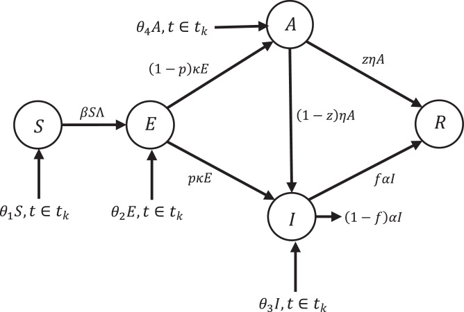
In this section, an impulsive SEIAR epidemic model is introduced due to sudden change that may occur for any reason, including travel and immigration for the whole population of the study area. Fig. 3 displays the diagram of impulsive SEIAR dynamic model. The dynamic of SEIAR model changes as follows:

$$\{\begin{array}{c}\dot{S}\left(t\right)=-\beta \Lambda \left(t\right)S\left(t\right)\\ \dot{E}\left(t\right)=\beta \Lambda \left(t\right)S\left(t\right)-\kappa E\left(t\right)\\ \dot{I}\left(t\right)=\left(1-z\right)\eta A\left(t\right)-\alpha I\left(t\right)+p\kappa E\left(t\right)\\ \dot{A}\left(t\right)=\left(1-p\right)\kappa E\left(t\right)-\eta A\left(t\right)\\ \dot{R}\left(t\right)=z\eta A\left(t\right)+f\alpha I\left(t\right)\end{array},t\notin t_k$$ (19-a)

$$\{\begin{array}{c}\dot{S}\left(t_k^{+}\right)=-\beta \Lambda \left(t\right)S\left(t\right)+{\theta }_1\left(t\right)S\left(t\right)\\ \dot{E}\left(t_k^{+}\right)=\beta \Lambda \left(t\right)S\left(t\right)-\kappa E\left(t\right)+{\theta }_2\left(t\right)E\left(t\right)\\ \dot{I}\left(t_k^{+}\right)=\left(1-z\right)\eta A\left(t\right)-\alpha I\left(t\right)+p\kappa E\left(t\right)+{\theta }_3\left(t\right)I\left(t\right)\\ \dot{A}\left(t_k^{+}\right)=\left(1-p\right)\kappa E\left(t\right)-\eta A\left(t\right)+{\theta }_4\left(t\right)A\left(t\right)\\ \dot{R}\left(t_k^{+}\right)=z\eta A\left(t\right)+f\alpha I\left(t\right)\end{array},t\in t_k$$ (19-b)

where t_k are integer numbers in which $k=1,2,\dots ,p,\dots$ and θ_i(t) which indicates the rate of new people being impulsively added to the population.

Remark 3:

Travel or immigration is the reason for this sudden change in population to groups (S, E, I, A) that is modeled as impulsive action in the model system. These individuals are added to the groups of the population once a day. In the real world, the people who are added include susceptible, infected, exposed and asymptomatic people. As a result, this population affects most of the groups and they add a population to each of these groups on a daily basis. The controller must also be able to counteract the effects of this sudden and daily increase in this population.

Fig. 3.

Conceptual flow diagram of impulsive SEIAR dynamic model.

4. The Optimal Control Problem of the Impulsive SQEIAR Epidemic Model

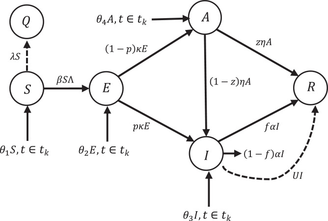
In this section, the controller design equations for the new model are modified. Also, Fig. 4 shows the applied controller on impulsive SQEIAR epidemic model. In this way, Eq. (19) is changed as follows:

$$\dot{S}\left(t\right)=-\left(\beta \Lambda \left(\mathrm{t}\right)+\lambda \left(t\right)\right)S\left(t\right)+\frac{t}{t}{\theta }_1\left(t\right)S\left(t\right)$$ (20-a)

$$\dot{Q}\left(t\right)=\lambda \left(t\right)S\left(t\right)$$ (20-b)

$$\dot{E}\left(t\right)=\beta S\left(t\right)\Lambda \left(t\right)-\kappa E\left(t\right)+\frac{t}{t}{\theta }_2\left(t\right)E\left(t\right)$$ (20-c)

$$\dot{I}\left(t\right)=\left(1-z\right)\eta A\left(t\right)-\alpha I\left(t\right)+p\kappa E\left(t\right)-U\left(t\right)I\left(t\right)+\frac{t}{t}{\theta }_3\left(t\right)I\left(t\right)$$ (20-d)

$$\dot{A}\left(t\right)=\left(1-p\right)\kappa E\left(t\right)-\eta A\left(t\right)++\frac{t}{t}{\theta }_4\left(t\right)A\left(t\right)$$ (20-e)

$$\dot{R}\left(t\right)=z\eta \mathrm{A}\left(t\right)+f\alpha I\left(t\right)+U\left(t\right)I\left(t\right)$$ (20-f)

such that  . is floor function. If t∉t_k (t_k indicates the day), then the term $\frac{t}{t}{\theta }_1\left(t\right)S\left(t\right)$ will be eliminated and if t ∈ t_k, term $\frac{t}{t}{\theta }_1\left(t\right)S\left(t\right)$ is added to the model as an impulsive. Similarly, this is true for Eqs. $\left(20-c\right)-\left(20-e\right)$.

Fig. 4.

Conceptual flow diagram of impulsive SQEIAR dynamic model with the proposed controller.

Similarly to the previous section, the problem is to minimize the cost function J that is written as Eq.3. So, the optimal controls are written as:

$$\begin{array}{ccc}\hfill U^{*}\left(t\right)& =& max\left\{min\left\{\frac{I^{*}\left(t\right)\left[p_4\left(t\right)-p_6\left(t\right)\right]}{A_5},U_{max}\right\},0\right\}\text{and}{\lambda }^{*}\left(t\right)\hfill \\ & & =max\left\{min\left\{\frac{S^{*}\left(t\right)\left[p_1\left(t\right)-p_2\left(t\right)\right]}{A_6},{\lambda }_{max}\right\},0\right\},\hfill \end{array}$$

therefore, the adjoint equation are also obtained as:

$$\begin{array}{ccc}& & {\dot{p}}_1\left(t\right)=-\frac{\partial H}{\partial S\left(t\right)}=-A_4\hfill \\ & & +\left(max\left\{min\left\{\frac{S^{*}\left(t\right)\left[p_1\left(t\right)-p_2\left(t\right)\right]}{A_6},{\lambda }_{max}\right\},0\right\}\right)\left[p_1\left(t\right)-p_2\left(t\right)\right]\hfill \\ & & -\frac{t}{t}{\theta }_1\left(t\right)p_1\left(t\right)\hfill \\ & & +\left(\beta \left(1-q\right)I^{*}\left(t\right)+\beta \epsilon E^{*}\left(t\right)+\beta \delta A^{*}\left(t\right)\right)\left[p_1\left(t\right)-p_3\left(t\right)\right]\hfill \end{array}$$ (21-a)

$${\dot{p}}_2\left(t\right)=-\frac{\partial H}{\partial Q\left(t\right)}=0$$ (21-b)

$$\begin{array}{ccc}& & {\dot{p}}_3\left(t\right)=-\frac{\partial H}{\partial E\left(t\right)}=-A_3+\beta \epsilon S^{*}\left(t\right)\left[p_1\left(t\right)-p_3\left(t\right)\right]\hfill \\ & & +\kappa \left[p_3\left(t\right)-p_5\left(t\right)\right]+p\kappa \left[p_5\left(t\right)-p_4\left(t\right)\right]-\frac{t}{t}{\theta }_2\left(t\right)p_3\left(t\right)\hfill \end{array}$$ (21-c)

$$\begin{array}{ccc}& & {\dot{p}}_4\left(t\right)=-\frac{\partial H}{\partial I\left(t\right)}=-A_1+\beta \left(1-q\right)S^{*}\left(t\right)\left[p_1\left(t\right)-p_3\left(t\right)\right]\hfill \\ & & +\alpha \left[p_4\left(t\right)-p_6\left(t\right)f\right]-\frac{t}{t}{\theta }_3\left(t\right)p_4\left(t\right)\hfill \\ & & +\left(max\left\{min\left\{\frac{I^{*}\left(t\right)\left[p_4\left(t\right)-p_6\left(t\right)\right]}{A_5},U_{max}\right\},0\right\}\right)\left[p_4\left(t\right)-p_6\left(t\right)\right]\hfill \end{array}$$ (21-d)

$$\begin{array}{ccc}& & {\dot{p}}_5\left(t\right)=-\frac{\partial H}{\partial A\left(t\right)}=-A_2+\eta \left[p_5\left(t\right)-p_4\left(t\right)\right]+z\eta \left[p_4\left(t\right)-p_6\left(t\right)\right]\hfill \\ & & +\beta \delta S^{*}\left(t\right)\left[p_1\left(t\right)-p_3\left(t\right)\right]-\frac{t}{t}{\theta }_4\left(t\right)p_5\left(t\right)\hfill \end{array}$$ (21-e)

$${\dot{p}}_6\left(t\right)=-\frac{\partial H}{\partial R\left(t\right)}=0$$ (21-f)

Remark 4:

According to $\dot{S}\left(t\right)=(-\beta \epsilon E\left(t\right)-\beta \left(1-q\right)I\left(t\right)-\beta \delta A\left(t\right)$ $-\lambda \left(t\right)+\frac{t}{t}{\theta }_1\left(t\right))S\left(t\right)$, if we can prove $(\beta \epsilon E\left(t\right)+\beta \left(1-q\right)I\left(t\right)+\beta \delta A\left(t\right)+\lambda \left(t\right))>\frac{t}{t}{\theta }_1\left(t\right)$ then, the change of S(t) is also decreasing and converges to zero.

Proof of Remark 4:

1. If t∉t_k then $\beta \epsilon E\left(t\right)+\beta \left(1-q\right)I\left(t\right)+\beta \delta A\left(t\right)+\lambda \left(t\right)>0$ fact that according to the positivity of parameters and states, is always true.2. If t ∈ t_k then $\beta \epsilon E\left(t\right)+\beta \left(1-q\right)I\left(t\right)+\beta \delta A\left(t\right)+\lambda \left(t\right)>{\theta }_1\left(t\right)$, since λ(t) is the control input and when needed, it can appear at its maximum value (0 ≤ λ(t) ≤ 1) then ${\lambda }_{max}\left(t\right)=1,$ So in the worst case, that the impulsive population add to the population the same size as the number of each group $\left({\theta }_1\left(t\right)={\theta }_{max}\left(t\right)=1\right)$ we can write $\beta \epsilon E\left(t\right)+\beta \left(1-q\right)I\left(t\right)+\beta \delta A\left(t\right)+1>1,$ given that the states and parameters are positive, $\beta \epsilon E\left(t\right)+\beta \left(1-q\right)I\left(t\right)+\beta \delta A\left(t\right)+\lambda \left(t\right)>{\theta }_1\left(t\right)$ is always true.Then change of S(t) is also decreasing and converges to zero.

Remark 5:

When S → 0 then Eq. (20-c) changes as:

$$\dot{E}\left(t\right)=\left(-k+\frac{t}{t}{\theta }_2\left(t\right)\right)E\left(t\right)$$ (22)

if we can prove $\sum _{forallt}k>\sum _{forallt}\frac{t}{t}{\theta }_2\left(t\right)$ then $\underset{t_1}{\overset{t_2}{\int }}\dot{E}\left(t\right)dt<0$ and $E\left(t_2\right)-E\left(t_1\right)<0$ also, since t ₂ > t ₁ (because t is time) then, the change of E(t) is decreasing and converges to zero E(t) → 0.

To proof of $\sum _{forallt}k>\sum _{forallt}\frac{t}{t}{\theta }_2\left(t\right)$, first, we suppose there is w′ (w′ ≥ 1) day and each day is divided into w (w ≥ 1) sections. Now the impact of the whole period is investigated:

Proof of Remark 5:

1. If

$$k>\frac{t}{t}{\theta }_2\left(t\right)$$ (23)

and knowing that in each part of a day (not a whole day, t∉t_k) then $\frac{t}{t}=0$, therefore, Eq. (23) changes to k > 0 and in every day (one single day, t ∈ t_k) then $\frac{t}{t}=1,$ therefore, Eq. (23) changes to k > θ ₂(t).

If we add up Eq. (23) for all t (t∉t_k and t ∈ t_k) for w′ days that we have w sections per day then we can write:

$$w^{\prime }kw>\sum _{i=1}^{w^{\prime }}{\theta }_2\left(i\right)$$ (24)

Eq. (24) can be written as:

$$k>\frac{{\sum }_{i=1}^{w^{\prime }}{\theta }_2\left(i\right)}{w^{\prime }w}$$ (25)

In the worst case $({\theta }_2\left(i\right)=1$ for all i) then $\sum _{i=1}^{w^{\prime }}{\theta }_2\left(i\right)=w^{\prime }$ and the Eq. (25) rewrite as:

$$k>\frac{w^{\prime }}{w^{\prime }w}=\frac{1}{w}$$ (26)

Since the SQEIAR dynamic is in continuous time, then the number of parts of a day is a large number w → ∞ then k > 0, that is always true. As a result, the Eq. (24) exist in whole period then it can be concluded that the change of E(t) is also decreasing and converges to zero. 2. If

$$k<\frac{t}{t}{\theta }_2\left(t\right)$$ (27)

We need to examine the validity of the following equation:

$$w^{\prime }kw<\sum _{i=1}^{w^{\prime }}{\theta }_2\left(i\right)$$ (28)

a) If ${\theta }_2\left(i\right)=0$ then $\sum _{i=1}^{w^{\prime }}{\theta }_2\left(i\right)=0$. Therefore, w′kw < 0, which is never true because of all three parameters are positive.

b) If ${\theta }_2\left(i\right)=1$ then $\sum _{i=1}^{w^{\prime }}{\theta }_2\left(i\right)=w^{\prime }$. Therefore, w′kw < w′, thereupon kw < 1 and since w → ∞ and k is positive, as a result, kw < 1 is never true.

From (a) and (b), Eq. (28) is not true.

So, it can be concluded, when Eq. (28) is not true then Eq. (24) is definitely and always true.

Remark 6:

As a result of this, the change of E(t) is also decreasing and converges to zero (E(t) → 0). Since, we proved the number of susceptible and exposed coverage to zero, therefore, the dynamics of the asymptomatic (Eq$.\left(20-e\right)$) changes as follows:

$$\dot{A}\left(t\right)=\left(-\eta +\frac{t}{t}{\theta }_4\left(t\right)\right)A\left(t\right)$$ (29)

in similar way, if $\eta >\frac{t}{t}{\theta }_4\left(t\right)$ or $\eta <\frac{t}{t}{\theta }_4\left(t\right)$, therefore, $w^{\prime }\eta w>\sum _{i=1}^{w^{\prime }}{\theta }_4\left(i\right)$ and the change of A(t) is also decreasing and converges to zero (A(t) → 0).

Remark 7:

Since A(t) and E(t) converged to zero then it is possible to deduce Eq. $\left(20-d\right)$ reformed as:

$$\dot{I}\left(t\right)=\left(-\alpha -U\left(t\right)+\frac{t}{t}{\theta }_3\left(t\right)\right)I\left(t\right)$$ (30)

If we can prove $\left(\alpha +U\left(t\right)\right)>\frac{t}{t}{\theta }_3\left(t\right)$ then, the change of I(t) is decreasing and converges to zero. In similar way for susceptible people:

Proof of Remark 7:

1. According to positivity of parameters, therefore, If t∉t_k then $\alpha +U\left(t\right)>0$. Therefore, this equation is always true.

2. If t ∈ t_k then $\alpha +U\left(t\right)>{\theta }_3\left(t\right)$.

Since U(t) is the control input and (0 ≤ U(t) ≤ 1) then $U_{max}\left(t\right)=1,$ So in the worst case $\left({\theta }_{max}\left(t\right)=1\right)$ we can write $\alpha +1>1$, therefore, this equation is always true.

We proved the number of infected (I), susceptible (S), exposed (E) converged to zero then the Eqs.$\left(20-b\right)$ and $\left(20-f\right)$ reformed as $\dot{Q}\left(t\right)=0,\dot{R}\left(t\right)=0$, it is noticeable that when the change of them is zero, then they remain on their maximum value.

After investigating the effect of the proposed controller on SQEIAR and impulsive SQEIAR model, we should simulate our result. Therefore, we outlined the results of our work in the next section as simulation result.

5. Simulation Results

In this section, a numerical result is given to corroborate the theoretical results presented in the two previous sections. Section 5.A illustrates the result of optimal control applied on the SQEIAR dynamic model while Section 5.B investigates the impact of the controller on sudden population change on this dynamic and presents the results. The initial parameter values of the SQEIAR epidemic model is shown in Table 1 and the model is applied to the case of SARS-Cov-2. Also, the values of the parameters in our epidemic model based on experimental data are from [25] and [26]. Some values ​​have changed based on the specific case of COVID-19 according to [2].

Table 2.

Parameters values of the SQEIAR epidemic model.

Parameter	Value
κ	0.54/day
α	0.3/day
η	0.3/day
p	0.1
f	0.965
ɛ	0
δ	1
q	0.5
z	0.02

Table 1.

Initial values of the SQEIAR epidemic model.

State variable	Initial value
S0	8000
Q0	0
E0	1000
I0	500
A0	500
R0	0
N0	10,000

A. Simulation Results of the SQEIAR Epidemic Model

The Figures below show the difference between the number of people from all of the groups in the both cases of absence and presence of the controller over the period shown. The plot of people without any control of them is illustrated in red, while the plot of people with control are shown in blue.

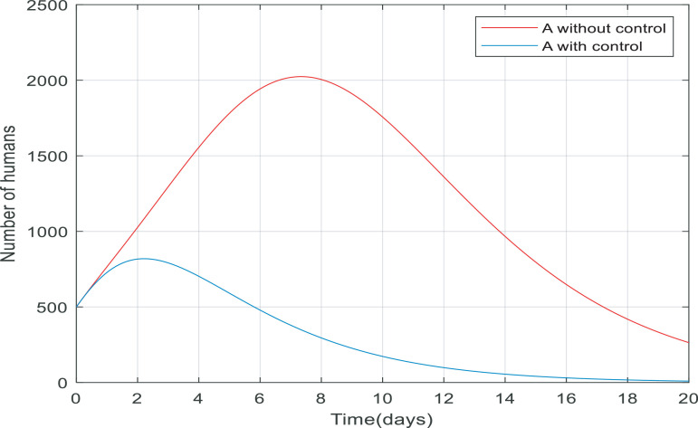
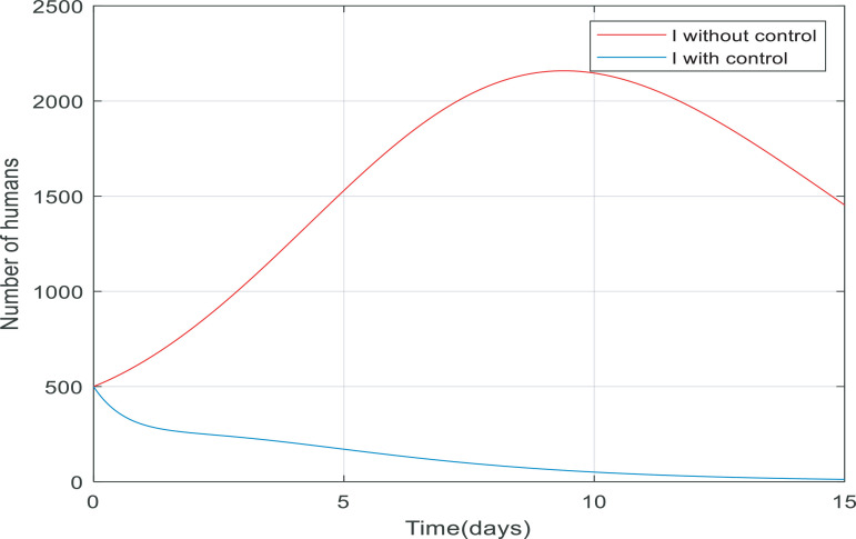
Fig. 5 compares the number of asymptomatic people without any control applied and the number of them with control (including quarantining the susceptible people and antiviral treatment of infected people). It is clear that the number of asymptomatic people decreased rapidly to zero (in approximately 20 day). Also, the peak difference between the number of people when the infection is uncontrolled by the time, we applied the controller on the dynamics is almost 1400. This indicates that the controller has been able to reduce the number of asymptomatic people involved. As shown in Fig. 6 the number of infected people increased from 500 to just over 2200 only in 10 days when there wasn't any control of them. But when we applied the controller, the infected people have also been going down and converge to zero in about 15 days, and the process of control has not caused to exceed the number of infected over 500.

Fig. 5.

Changes in population number of asymptomatic individuals over time with and without control.

Fig. 6.

Changes in population number of infected individuals over time with and without control.

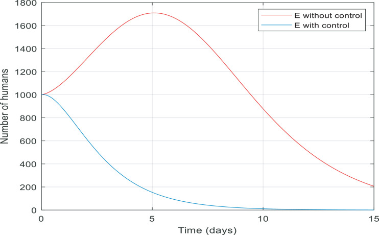
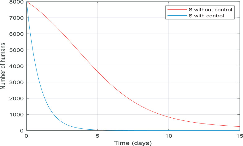
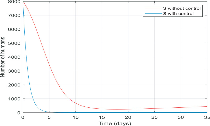
In Fig. 7 , from the first day to day five, there was a big increase in the number of exposed people. By contrast, there was a big fall in the number of them controlled by the proposed controller in almost ten days. Fig. 8 gives information about the number of susceptible people with and without control in 15 days. It is noticeable that control the infection by quarantining susceptible people has been effective, therefore, the number of susceptible people fell by 8000 to zero in around five days.

Fig. 7.

Changes in population number of exposed individuals over time with and without control.

Fig. 8.

Changes in population number of susceptible individuals over time with and without control.

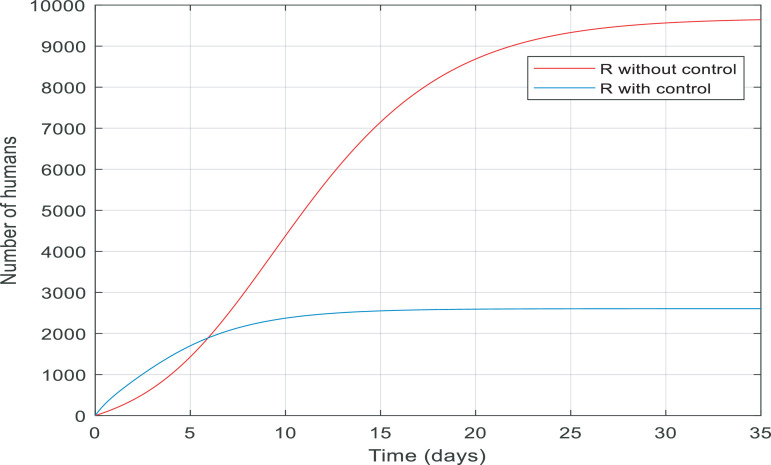
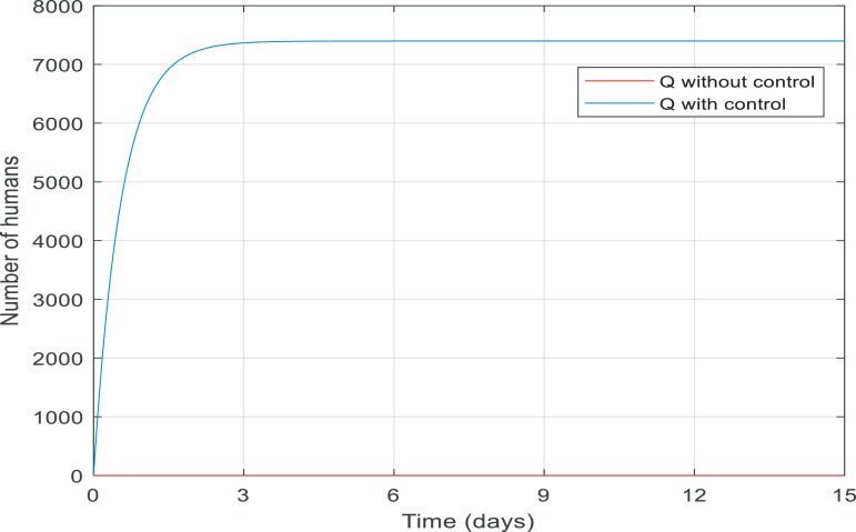
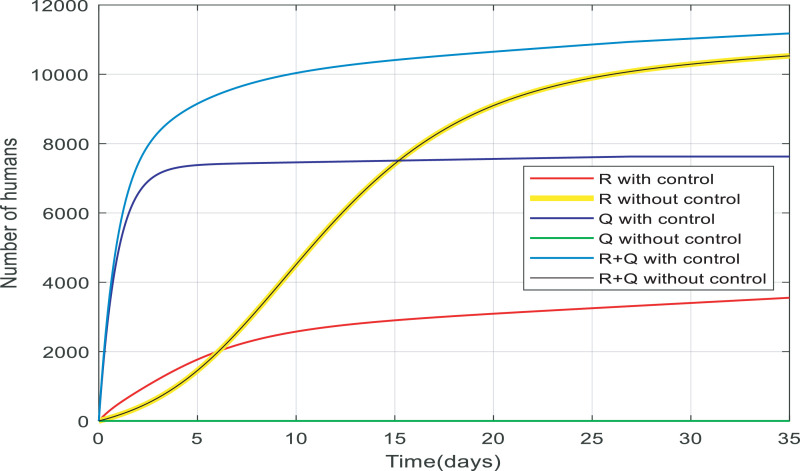
Fig. 9 compares the number of recovered individuals with and without the applied controller. We can see a decrease in the number of recovered individuals with the controller over the 35-day period. It is noticeable that in almost 15 days only about 2500 of them are recovered and remained at 2500. The reason for this is obvious because when people are quarantined against the infection, fewer people will get infected then fewer people will recover which is discussed in greater detail in Fig. 13. Fig. 10 also shows when there was no control over the infection, the number of quarantined individuals was zero and with the control of them, the number gradually increases, which is normal.

Fig. 9.

Changes in population number of recovered individuals over time with and without control.

Fig. 13.

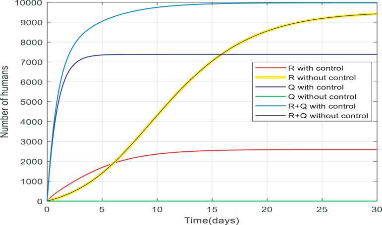
Comparison between the recovered and quarantined individuals and a total of them with and without control.

Fig. 10.

Changes in population number of quarantined individuals over time with and without control.

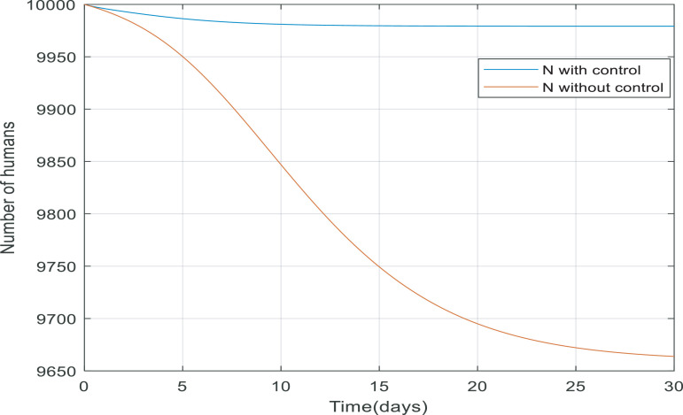
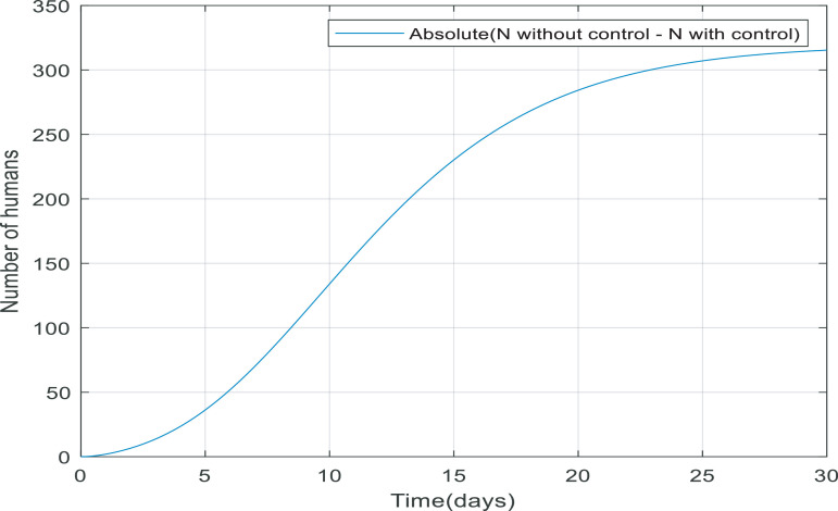
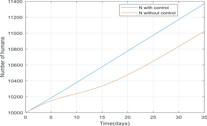
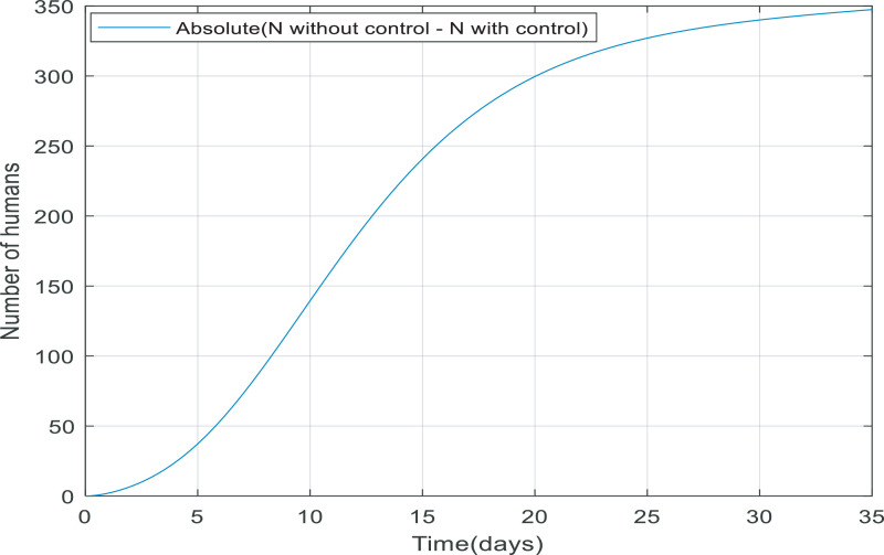
Looking at Fig. 11 , when the controller applied to the dynamic, more people survive because the total number of the population equals the number of recovered and quarantined people. The reason that the total number of people is not exactly equal to 10,000 people is that 3.5% of infected people die from their infection. Fig. 12 shows the absolute difference between N(t) with and without the controller, it can conclude the difference between them reaches to a constant value (approximately 315), meaning the controller has managed to keep 315 more people alive.

Fig. 11.

Changes in total number of populations over time with and without control.

Fig. 12.

Comparison between total population (N(t)) with and without the controller.

In Fig. 13 , there are two separate cases: with no control and with control. In the case of people under control, more than half of the recovered people went down while quarantined people are almost 7200, therefore a total of them is approximately 10,000(≅9970). It is noticeable that the majority of susceptible people are quarantined and there are fewer infected people to become recovered. While in the case of people without the controller the number of recovered people rose to around 9660 and there are any quarantined people, therefore, a total of them is about 9660. as a result, the total number of alive people with control is more than the case without control. Approximately 200 more people have survived from infection when the infection is under control which is very significant in a community of 10,000 people.

B. Simulation Results of the Impulsive SQEIAR Epidemic Model

The following figures compare the number of people from different groups introduced before with and without the controller. The difference between these figures and the figures of Section 5.A is that in this section, some people are being added at variable rates θ_i(t) to susceptible, exposed, infected and asymptomatic individuals every day. This fact means the number of these people will never be zero but the controller has been able to overcome this population growth and eradicate the disease.

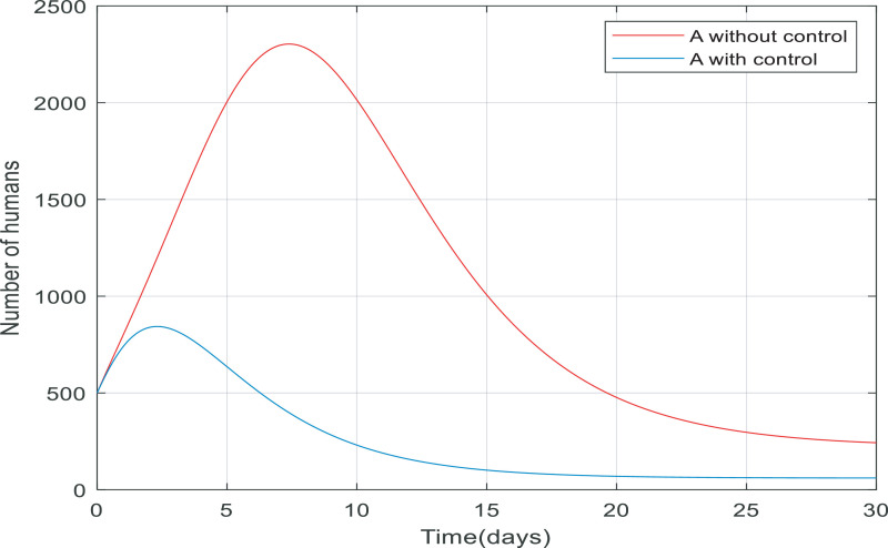
There is a number of asymptomatic people that is added to the asymptomatic group of travelers and migrants entering the society every day at variable rates and they do not allow declining the population of asymptomatic individuals. They are also causing the epidemic to continue, so with proper and optimal control, we must prevent it from spreading in the community. Fig. 14 illustrates the number of asymptomatic people decreasing daily and it eventually reaches 250 and remains stable. This is because populations that come into society every day change suddenly and prevent this decline. On the other hand, the blue line shows that the controller has been able to overcome this population stagnation and reduce their numbers.

Fig. 14.

Time evolution of asymptomatic people with and without controls with the impulsive rate of growth.

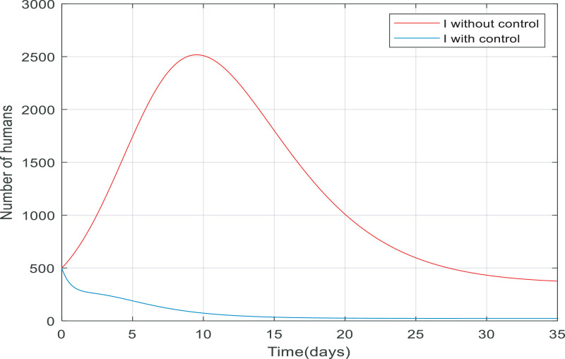
Since those who are added to the society (by travel or immigration) also include the infected individuals which cause the outbreak, daily injections of people on to the whole population under study have a profound effect on the number of infected people too. The controller was also able to reduce the number of infected people because if the infected population was not controlled, approximately 500 people in the community would infect and spread the disease daily. But the reason for the population staying constant is that as infected people are added to the population daily, some of them recover and go to the recovered group and some die from the infection then the population almost reaches stability and remains constant that is controlled by the controller, and finally the number of infected people has fallen to zero shown in Fig. 15 .

Fig. 15.

Time evolution of infected people with and without controls with the impulsive rate of growth.

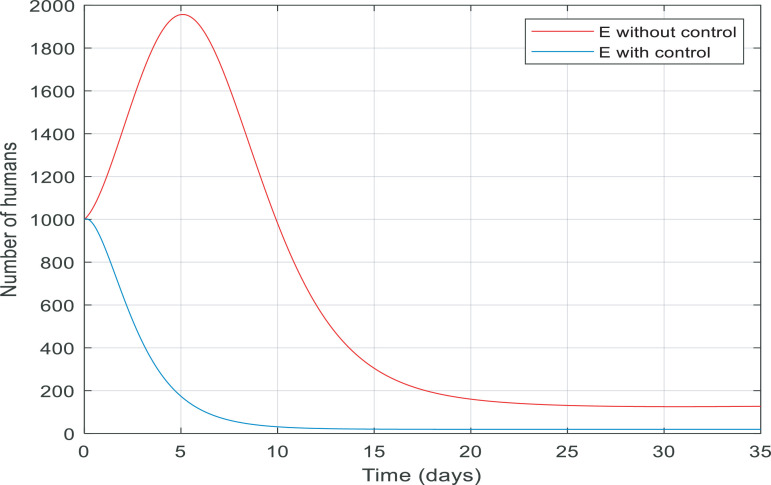
In Figs. 16 and 17 , it can be observed the impact of the sudden population increase on the number of exposed and susceptible individuals, respectively. The controller reduced the population of susceptible individuals to zero within five days and the population of exposed individuals to the lowest possible extent.

Fig. 16.

Time evolution of exposed people with and without controls with the impulsive rate of growth.

Fig. 17.

Time evolution of susceptible people with and without controls with the impulsive rate of growth.

As previously mentioned, the number of individuals in quarantine is equal to zero when there is no control over the disease, but when we implement the controller, the number of people in quarantine increases. It is noticeable in Fig. 13 that the number of people in quarantine when no population enters the community is approximately 7200, but in Fig. 18 when people come into the community that included susceptible people too, the same number must also be quarantined daily. Thus, there was about 700 increase in numbers and the number of people in quarantine went up to approximately under 8000. The number of recovered people has also increased compared to the time when there was no sudden injection of the population because those who enter the community include infected people who go to the recovered group after the recovery and increase the number of recovered people. While some people are adding to the population and there is no control over it, the number of recovered people is greater than when the population is controlled because in a controlled case, because the susceptible individuals are rapidly quarantined and fewer people get infected and eventually recover. The total number of people in the quarantine plus the recovered ones in the controlled case is higher because in the uncontrolled case there were no quarantined people at all, but in the controlled case, the people in the quarantine are all healthy and have a large share in society. The reason for the daily increase in the $R\left(t\right)+Q\left(t\right)$ plot is that the population of the community is dynamic, not closed and a number is added to the population every day. $\left(\dot{N}\left(t\right)\ne 0\right)$

Fig. 18.

Time evolution of recovered and quarantined people and a total of them with and without controls with the impulsive rate of growth.

Fig. 19 shows the number of changes in the total population size each day when there is no control over dynamic compared with the number of them under proposed optimal control. As shown, we were able to keep more of the population alive with the controller compared with when the infection was spreading without any control. Fig. 20 shows the absolute difference between the whole population with and without the controller. The difference between them is a constant value (equal to 350), meaning the controller has managed to keep 350 more people alive per unit of time.

Fig. 19.

Time evolution of total population of people with and without controls with the impulsive rate of growth.

Fig. 20.

The absolute of total population of people with and without controls with the impulsive rate of growth.

6. Comparison with other Diseases and with Actual Data

This section is divided into four sub-section, in the first and second sub-section (A and B, respectively), the results of the controller applied to the impulsive epidemic model are compared for two different diseases (Ebola Virus Disease (EVD) and influenza). In the following sub-section C, the simulation result for three types of diseases (COVID-19, Ebola, and Influenza) are compared together. Finally, the comparison of simulation results with real data of China and Spain is also given in the last sub-section. The parameters of each disease are represented in Table 3 .

Table 3.

Parameters values of the SQEIAR epidemic model.

Parameter	Ebola [27]	Influenza(H2N2) [24]	COVID-19
κ	0.0023	0.526	0.54
α	0.178	0.244	0.3
η	0.178	0.244	0.3
p	0.76	0.667	0.1
f	0.26	0.98	0.965
ɛ	0	0	0
δ	1	1	1
q	0.5	0.5	0.5
z	0.02	0.9	0.02

A. Ebola Virus Disease (EVD)

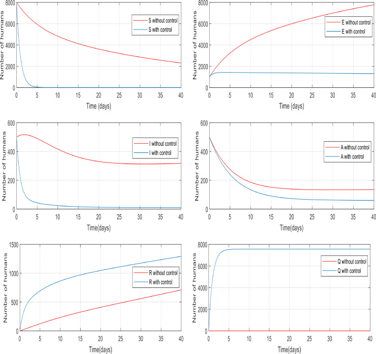
As it can be seen in Fig. 21 , the number of susceptible people is reduced in only 5 days when the controller is applied to the impulsive epidemic model. There is a big fall in the number of exposed people when the controller is applied to the dynamic and this reduction is acceptable for Ebola disease because the rate of (κ) is low, that is, the exposed people, go to the infected and asymptomatic group at a lower rate. Also, since the population is considered dynamic, some people are added every day (whether traveling or migrating) and it prevents the population of groups from declining rapidly. Despite the Ebola virus disease is a severe, often fatal illness in humans and its case fatality rate is 90% the controller was still able to reduce the number of infected significantly. When recovered people were controlled, the number of them is increased by almost 550 people and reached to almost 1300 in 40 days.

Fig. 21.

The Comparison between (S(t), Q(t), E(t), I(t), A(t), R(t)) with and without the controller in Ebola.

B. Influenza (H2N2)

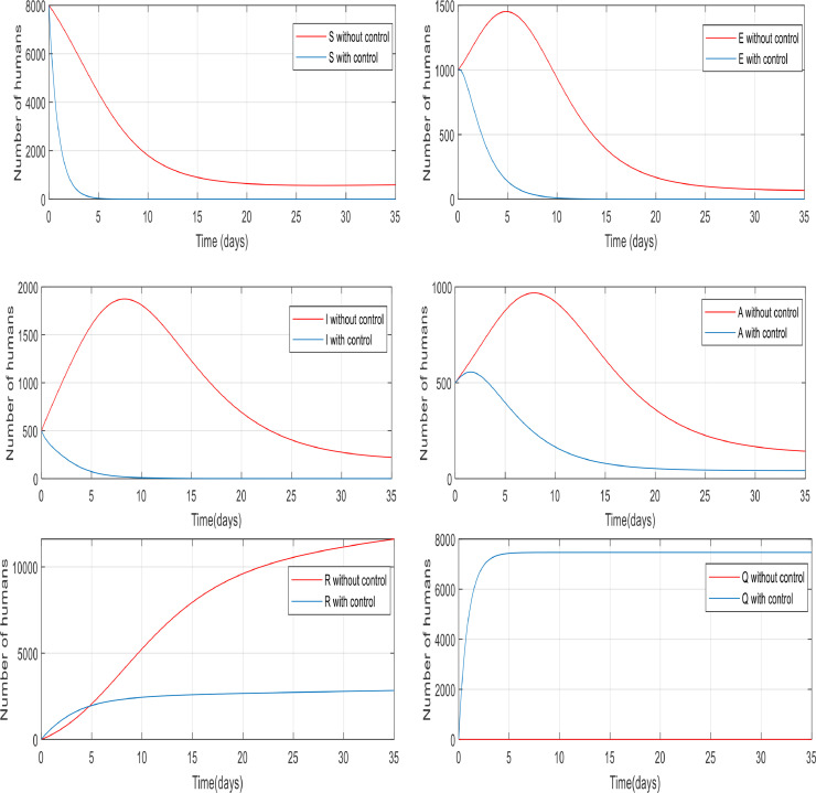
According to Fig. 22 and as stated in detail in the preceding sections, the controller was able to properly control the susceptible individuals and move them to the quarantined people group. Also, the number of infected and exposed people converged to zero in only 10 days with the controller. The number of asymptomatic people with the controller has also reached its lowest level and the reason it takes longer to reach zero is that there is no direct controller on it and zeroing of this is as a result of zeroing of the other groups, which are discussed in detail in Remark 6. Recovered people in the presence of controller are reduced compared to when there was no control over them because when there is no control over the disease, the number of infected people is higher, so the number of recovered will be more, also the death rate in influenza is less than Ebola. In the end, the number of people in quarantine with controllers has reached its peak.

Fig. 22.

The Comparison between (S(t), Q(t), E(t), I(t), A(t), R(t)) with and without the controller in Influenza.

C. Comparison of Three Types of Diseases (COVID-19, Ebola, and Influenza)

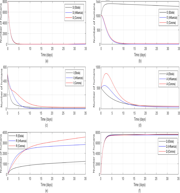
As it can be seen in Fig. 23. a, the controller was able to control the dynamic and the susceptible individuals are quarantined in all three disease groups. In Fig. 23.b, the number of exposed people in both influenza and corona groups are converged to zero by the controller in ten days. But the number of exposed people in the Ebola disease group is reached to zero later because the rate of κ in this disease is lower than the other group and prevents exposed individuals from joining groups A and I rapidly. In Remark 5, it is proved that E eventually reaches zero. Fig. 23.c shows the number of infected people went down by controller and according to Fig. 23.d in every three groups, the number of asymptomatic people converged to zero later because there was no direct controller on them, but in the end, according to the evidence in Remark 6, they eventually got to zero. Since exposed people have a higher rate of infection (κ) in coronavirus (according to Table 3), so more of them get infected and eventually more of them will be recovered, which is quite evident in Fig. 23.e. The number of recovered people in Ebola is lower than the other two groups, this reduction is acceptable for Ebola disease because the mortality rate (f) is very high therefore there are fewer infected people, as a result, fewer recovered people. Finally, in Fig. 23.f, the susceptible individuals are well quarantined and the number of people in the quarantine group is increased.

Fig. 23.

The comparison between different groups of people in one community against three types of disease like Influenza, Coronavirus, and Ebola (S(t), Q(t), E(t), I(t), A(t), R(t)).

D. Comparison of the Simulation Results with Actual Data of China and Spain

In this sub-section, divided into two prats (1 and 2), the accuracy of the designed controller is examined by the actual data of China. Then, the controller, whose parameters were estimated using actual data of China, is applied to the actual data of Spain to show the applicability of quarantine and treatment policies in both countries.

China

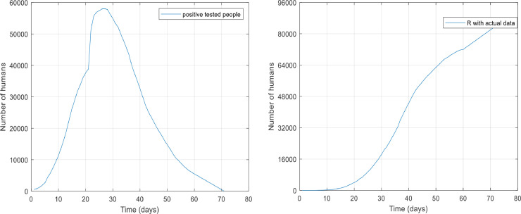
To evaluate the SQEIAR epidemic model, we need to study a successful model of this type of operation (quarantine and treatment). China has been one of those countries involved with the virus that has been able to control and eventually eradicate it. Therefore, in this part, the results of this study are compared to the actual data from China, to find out the efficiency of the designed controller. If we look at the total population of cities infected with coronavirus in China, they are approximately 80,000,000 people. The number of those who have tested positive for the coronavirus and recovered people given by the National Health Commission of the People's Republic of China (from 22 January 2020 to 22 March 2020) [28] shown in Fig. 24 respectively. According to [29], about 20% of those who have tested positive for the coronavirus have no symptoms of the disease (asymptomatic people) and the rest of them are infected.

Fig. 24.

The number of people who has tested positive for the virus and recovered people in China.

Using this real data, the number of other states can be estimated. Since R ₀ (Basic Reproduction Number [3, 30]) equal to 2 then the value of E(t) can be calculated as $E\left(t\right)\approx 2I\left(t\right)+2A\left(t\right)$, that is, each person whether asymptomatic or infected can infect two other people and by assuming 98% of people are quarantined, the number of susceptible people can easily be calculated as $S\left(t\right)=N\left(t\right)-Q\left(t\right)-E\left(t\right)-I\left(t\right)-A\left(t\right)-R\left(t\right)$.

If the model output is considered as the total number of quarantined and recovered people, therefore, the parameters of the system can be identified by actual data given from [27]. For this purpose, we consider $y\left(t\right)=\left[\begin{array}{cccccc}0& 1& 0& 0& 0& 1\end{array}\right]{\left[\begin{array}{ccccc}S\left(t\right)& Q\left(t\right)& E\left(t\right)I\left(t\right)& A\left(t\right)& R\left(t\right)\end{array}\right]}^T$ which implies $y\left(t\right)=Q\left(t\right)+R\left(t\right)$. By using Eq. $\left(2-b\right)$, $\dot{Q}\left(t\right)=\lambda \left(t\right)S\left(t\right)$that is equivalent to $\frac{dQ\left(t\right)}{dt}=\lambda \left(t\right)S\left(t\right)$ and then $dQ\left(t\right)=\lambda \left(t\right)S\left(t\right)dt$ and $\underset{0}{\overset{t}{\int }}dQ\left(t\right)=\underset{0}{\overset{t}{\int }}\lambda \left(t\right)S\left(t\right)dt$. By assuming λ is stationary, then $Q\left(t\right)-Q\left(0\right)=\lambda \underset{0}{\overset{t}{\int }}S\left(t\right)dt$. Since $Q\left(0\right)=0$ then finally $Q\left(t\right)=\lambda \underset{0}{\overset{t}{\int }}S\left(t\right)dt$. In the same way and by assuming U is stationary, since $\dot{R}\left(t\right)=z\eta \mathrm{A}\left(t\right)+\left(f\alpha +U\right)I\left(t\right)$ then $R\left(t\right)=z\eta \underset{0}{\overset{t}{\int }}A\left(t\right)dt+\left(f\alpha +U\right)\underset{0}{\overset{t}{\int }}I\left(t\right)dt$. Since the actual data used reported daily, then the model is changed to a discrete-time model. By this fact it can be deduced

$$y_k=z\eta \sum _{i=0}^k{A}_i+\left(f\alpha +U\right)\sum _{i=0}^k{I}_i+\lambda \sum _{i=0}^k{S}_i$$ (31)

where y_k is the output of kth day, therefore:

$$y_k=\left[\begin{array}{ccc}\sum _{i=0}^k{A}_i& \sum _{i=0}^k{I}_i& \sum _{i=0}^k{S}_i\end{array}\right]\left[\begin{array}{c}z\eta \\ f\alpha +U\\ \lambda \end{array}\right]$$ (32)

Define the parameter vectors θ, and the information vectors φ_k as $\theta ={\left[\begin{array}{ccc}{\theta }_1& {\theta }_2& {\theta }_3\end{array}\right]}^T={\left[\begin{array}{ccc}z\eta & f\alpha +U& \lambda \end{array}\right]}^T$ and ${\phi }_k={\left[\begin{array}{ccc}{\phi }_1& {\phi }_2& {\phi }_3\end{array}\right]}^T={\left[\begin{array}{ccc}\sum _{i=0}^k{A}_i& \sum _{i=0}^k{I}_i& \sum _{i=0}^k{S}_i\end{array}\right]}^T$, respectively. We obtain the following evaluations:

$$y_k={\phi }_k^T\theta$$ (33)

define a quadratic criterion function:

$$J\left(\theta \right)=\sum _{k=0}^{\aleph }{\left[e_k\right]}^2=\sum _{k=0}^{\aleph }{\left[y_i-{{\phi }_k}^T\theta \right]}^2={\left(Y_k-{\Phi }_k\theta \right)}^T\left(Y_k-{\Phi }_k\theta \right)$$ (34)

where ℵ is the total number of samples and the vector Y_k and the matrix Φ_k are defined as $Y=\left[\begin{array}{c}\begin{array}{c}{y}_1\\ y_2\\ ⋮\end{array}\\ y_{\aleph }\end{array}\right]\in {\mathbb{R}}^{\aleph }$ and $\Phi =\left[\begin{array}{c}\begin{array}{c}{{\phi }_1}^T\\ {{\phi }_2}^T\\ ⋮\end{array}\\ {{\phi }_{\aleph }}^T\end{array}\right]\in {\mathbb{R}}^{\aleph \times 3}$. By minimizing the criterion function J, the least-squares estimate of θ is obtained as:

$$\theta ={\left({\Phi }^T\Phi \right)}^{-1}{\Phi }^{T}Y$$ (35)

However, since Φ and Y are known, it is possible to calculate the parameter estimation vector θ via the above equation directly. Replacing the obtained parameters in the model of this study and comparing the responses, the following results are obtained. If new data is added to the system while system is estimating at the same time, it should be used recursive Identification as described in detail [31].

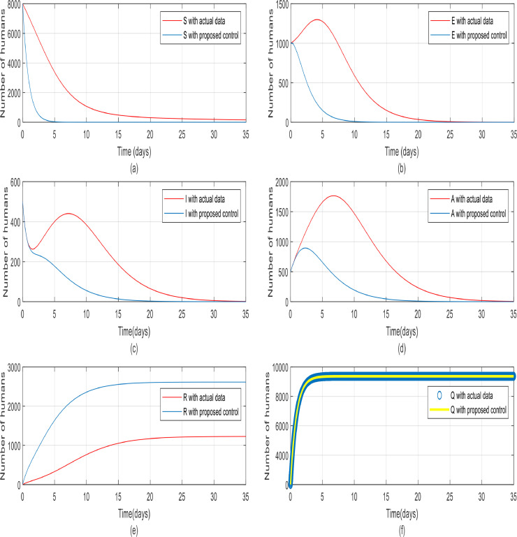
As seen in Fig. 25 , the results of applying the controller on the original model are compared to a model whose parameters are estimated using real data, and the total number is scaled for a population of 10,000. In part (a), when the controller is applied to the model using the identified parameters, the rate of reduction of the susceptible individuals is lower than before (when the controller is applied to the original model), which is also justified in reality but ultimately achieved zero. Part (b) shows the diagram of the exposed people, when the model parameters were identified by using real data, initially had a peak, but the controller converged it to zero in about twenty days. Part (c) of Fig. 25 shows that unlike quarantine and treatment in the real-world, the peak in the number of infected people does not show up in modeling, but eventually converges to zero. In part (d), similar to part (c), the diagrams of the asymptomatic population have a higher peak than people in the modeling, and have growth about 1800 in population, but have finally become zero by the 30th day. A valid point can be found in part (e) is the reduction in the population of recovered people (with real data) and the reason for this is that the recovery time is actually longer and more delayed in real-world society. Part (f) shows the quarantine of individuals at a rate of 98 percent, which is equal in both cases, and 98 percent of the total population (10,000) are quarantined successfully. As can be seen from the results of these studies and since China, where the virus originated from, have implemented quarantines and got good results and also quarantine is by far one of the most effective ways to prevent the spread of the disease like coronavirus that there is still no vaccine for them. So, it is concluded that without the quarantine, the disease spreads very rapidly and will be highly fatal and catastrophic.

Fig. 25.

The comparison between different groups of people in one community with proposed control and actual data (S(t), Q(t), E(t), I(t), A(t), R(t)).

Spain

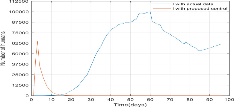
In this part, similar to part 1 process, the results obtained from applying the desired controller to the disease and the actual data are compared. In part 1, unknown parameters are estimated using real data from China. In Fig. 26 , 2 diagrams are compared. The diagram in blue shows the number of confirmed cases in Spain, which is based on actual data, extracted from the Health Alert and Emergency Coordination center (from 24 Feb to 29 May 2020) [32]. The red graph shows the number of declining trends in the number of infected people when the controller is applied. The controller parameters are estimated by the actual data from China. As it is known, if Spain had taken the process of controlling the COVID-19, it could have controlled the disease well and within about 20 days. In the case that the desired controller applied to the model, the number of infected people has finally reached approximately 62,500, but in the case without the controller, the number of infected people has reached 100,000 and has an upward trend after 85 days, which has reached zero in the shortest time in the controlled case. It is essential to note that the evidence in this paper, given from modeling studies, proves how quarantine affects the COVID-19 outbreak. Putting quarantine in place early and combining it with medical treatment is critical if it is to be effective to control the spread of COVID-19. Also, the quarantining of travelers from a country involved with COVID-19 reduces disease transmission and deaths and also makes greater cost-savings. However, if the government enact strict laws to ban rallies and quarantine and other different ways to getting people away from rallies like: Isolation, social distancing, community containment, driving ban and etc., in the shortest possible time, it can be expected that the COVID-19 prevalence will decline in the next few months.

Fig. 26.

The comparison between the number of infected people in Spain with and without proposed controller.

7. Conclusion

In this paper, the SEIAR dynamic epidemic model was improved with a new group of people called quarantined people (SQEIAR). The goal of this article was to eradicate the infection by decreasing the number of infected, exposed, and asymptomatic and quarantining the susceptible people with optimal control that applied to the SQEIAR model. Two control actions are employed to achieve this objective: quarantine and treatment of infected individuals. The Pontryagin's maximum principle was used to describe the optimal controls and the optimal final time. Also, an impulsive epidemic model was considered to indicate the sudden growth in population and that model was controlled by optimal control strategy. The presented approach is suitable to describe models for infectious diseases caused by a group of viruses called coronavirus for which there is no vaccine yet. Thus, the theoretical results were illustrated for the case of COVID-19. Our simulation results of the COVID-19 were compared with Ebola and Influenza. Also, numerical simulation corroborated our theoretical results. Then, the system parameters were identified using actual data of China. Eventually, the process of quarantine and treatment of China and Spain was compared by applying the controller with the estimated parameters using actual data of China.

Declaration of Competing Interest

None.

References

- 1.Tahir M., Shah S.I.A., Zaman G., Khan T. ‘ Prevention Strategies for Mathematical Model MERS-Corona Virus with Stability Analysis and Optimal Control’. Journal of Nanoscience and Nanotechnology, 2018;2:401. [Google Scholar]
- 2.‘World Health Organization (WHO) 2020. Coronavirus’. [Google Scholar]
- 3.Amiri Mehra, A.H., Zamani I., Abbasi Z., Ibeas A. ‘Observer-Based Adaptive PI Sliding Mode Control of Developed Uncertain SEIAR Influenza Epidemic Model Considering Dynamic Population’. Journal of Theoretical Biology, 2019;482 doi: 10.1016/j.jtbi.2019.08.015. [DOI] [PubMed] [Google Scholar]
- 4.Ibeas A., de la Sen M., Alonso-Quesada S., Zamani I. ‘Stability Analysis and Observer Design for Discrete-Time SEIR Epidemic Models’. Advances in Difference Equations, 2015;2015(1):122. [Google Scholar]
- 5.Ibeas A., de la Sen M., Alonso-Quesada S., Zamani I., Shafiee M. Observer Design for SEIR Discrete-Time Epidemic Models'. in 2014 13th International Conference on Control Automation Robotics & Vision; ICARCV; 2014. pp. 1321–1326. [Google Scholar]
- 6.Zamani I., Shafiee M. ‘Stability Analysis of Uncertain Switched Singular Time‐Delay Systems with Discrete and Distributed Delays’. Optimal Control Applications Methods, 2015;36(1):1–28. [Google Scholar]
- 7.Jana S., Haldar P., Kar T. ‘Optimal Control and Stability Analysis of an Epidemic Model with Population Dispersal’, Chaos. Chaos, Solitons & Fractals, 2016;83:67–81. [Google Scholar]
- 8.Zhang T., Teng Z. ‘An Impulsive Delayed SEIRS Epidemic Model with Saturation Incidence’. Journal of Biological Dynamics, 2008;2(1):64–84. doi: 10.1080/17513750801894845. [DOI] [PubMed] [Google Scholar]
- 9.Meng X., Li Z., Wang X. ‘Dynamics of a Novel Nonlinear SIR Model with Double Epidemic Hypothesis and Impulsive Effects’. Journal of Biological Dynamics, 2010;59(3):503–513. doi: 10.1007/s11071-009-9557-1. [DOI] [PMC free article] [PubMed] [Google Scholar]
- 10.Jia Q., Xia C... ‘Exponential Stability of Impulsive Delayed Nonlinear Hybrid Differential Systems’. Archives of Electrical Engineering, 2019;68(3) [Google Scholar]
- 11.Zamani I., Shafiee M., Ibeas A., de la Sen M. in AIP Conference Proceedings. Vol. 1637. 2014. 'Switched Impulsive Control of the Endocrine Disruptor Diethylstilbestrol Singular Model'; pp. 1218–1227. American Institute of Physics. [Google Scholar]
- 12.Zamani I., Shafie M. in 2009 IEEE International Conference on Fuzzy Systems. 2009. 'Fuzzy Affine Impulsive Controller'; pp. 361–366. [Google Scholar]
- 13.Zamani I., Shafiee M., Ibeas A. ‘On Singular Hybrid Switched and Impulsive Systems’. International Journal of Robust Nonlinear Control, 2018;28(2):437–465. [Google Scholar]
- 14.Zamani I., Shafie M. in 2009 IEEE International Conference on Fuzzy Systems. 2009. 'Fuzzy Impulsive Control with Application to Chaos Control'; pp. 338–343. [Google Scholar]
- 15.Stengel R.F., Ghigliazza R., Kulkarni N., Laplace O. ‘Optimal Control of Innate Immune Response’. Optimal Control Applications and Methods, 2002;23(2):91–104. [Google Scholar]
- 16.Lhous M., Rachik M., Larrache A. ‘Free Optimal Time Control Problem for a SEIR-Epidemic Model with Immigration of Infective’. International Journal of Computer Applications, 2017;159(3):1–5. [Google Scholar]
- 17.Abdelhadi A., Hassan L. ‘Optimal Control Strategy for SEIR with Latent Period and a Saturated Incidence Rate’. ISRN Applied Mathematics, 2013;2013 [Google Scholar]
- 18.Zamani, I., Zaynali, M., Shafiee, M., Afshar, A.: 'Optimal Control of Singular Large-Scale Linear Systems', in 2011 19th Iranian Conference on Electrical Engineering, 2011, pp. 1–5.
- 19.Di Giamberardino P., Iacoviello D. ‘Optimal Control of SIR Epidemic Model with State Dependent Switching Cost Index’. Biomedical Signal Processing and Control, 2017;31:377–380. [Google Scholar]
- 20.Sharomi O., Malik T. ‘Optimal Control in Epidemiology’. Annals of Operations Research, 2017;251(1–2):55–71. [Google Scholar]
- 21.Rachah A. ‘Analysis, Simulation and Optimal Control of a SEIR Model for Ebola Virus with Demographic Effects’. Communications Faculty of Sciences University of Ankara Series A1 Mathematics and Statistics. 2018;67(1):179–197. [Google Scholar]
- 22.Area, I., NdaÏrou, F., Nieto, J.J., Silva, C.J., Torres, D.: 'Ebola Model and Optimal Control with Vaccination Constraints', arXiv, 2017.
- 23.Zamani I., Shafiee M., Shafieirad M., Zeinali M. ‘Optimal Control of Large-Scale Singular Linear Systems Via Hierarchical Strategy’. Transactions of the Institute of Measurement Control, 2019;41(8):2250–2267. [Google Scholar]
- 24.Arino J., Brauer F., Van Den Driessche P., Watmough J., Wu J. ‘A Model for Influenza with Vaccination and Antiviral Treatment’. Journal of Theoretical Biology, 2008;253(1):118–130. doi: 10.1016/j.jtbi.2008.02.026. [DOI] [PubMed] [Google Scholar]
- 25.Riou J., Althaus C.L. ’Pattern of Early Human-to-Human Transmission of Wuhan 2019 Novel Coronavirus (2019-nCoV), December 2019 to January 2020. Eurosurveillance, 2020;25(4) doi: 10.2807/1560-7917.ES.2020.25.4.2000058. [DOI] [PMC free article] [PubMed] [Google Scholar]
- 26.Li Q., Guan X., Wu P., Wang X., Zhou L., Tong Y., et al. ‘Early Transmission Dynamics in Wuhan, China, of Novel Coronavirus–Infected Pneumonia’. The New England Journal of Medicine, 2020 doi: 10.1056/NEJMoa2001316. [DOI] [PMC free article] [PubMed] [Google Scholar]
- 27.Althaus C.L. ‘Estimating the Reproduction Number of Ebola Virus (EBOV) During the 2014 Outbreak in West Africa’. PLoS Currents, 2014:6. doi: 10.1371/currents.outbreaks.91afb5e0f279e7f29e7056095255b288. [DOI] [PMC free article] [PubMed] [Google Scholar]
- 28.'National Health Commission of the People's Republic of China (NHC)', 2020. [DOI] [PMC free article] [PubMed]
- 29.Mizumoto K., Kagaya K., Zarebski A., Chowell G. ’Estimating the Asymptomatic Proportion of Coronavirus Disease 2019 (COVID-19) Cases on Board the Diamond Princess Cruise Ship, Yokohama, Japan, 2020′. Eurosurveillance, 2020;25(10) doi: 10.2807/1560-7917.ES.2020.25.10.2000180. [DOI] [PMC free article] [PubMed] [Google Scholar]
- 30.Van den Driessche P., Watmough J. ‘Reproduction Numbers and Sub-Threshold Endemic Equilibria For Compartmental Models of Disease Transmission’. Mathematical Biosciences, 2002;180(1):29–48. doi: 10.1016/s0025-5564(02)00108-6. [DOI] [PubMed] [Google Scholar]
- 31.Shafieirad M., Shafiee M., Abedi M. ‘Recursive Identification of Continuous Two-Dimensional Systems in the Presence of Additive Colored Noise’. IETE Journal of Research, 2014;60(1):74–84. [Google Scholar]
- 32.‘Health Alert and Emergency Coordination Centre’ . 2020. [Google Scholar]