Practical considerations for measuring the effective reproductive number, R_t

Abstract

Estimation of the effective reproductive number, R_t, is important for detecting changes in disease transmission over time. During the COVID-19 pandemic, policymakers and public health officials are using R_t to assess the effectiveness of interventions and to inform policy. However, estimation of R_t from available data presents several challenges, with critical implications for the interpretation of the course of the pandemic. The purpose of this document is to summarize these challenges, illustrate them with examples from synthetic data, and, where possible, make methodological recommendations. For near real-time estimation of R_t, we recommend the approach of Cori et al. (2013), which uses data from before time t and empirical estimates of the distribution of time between infections. Methods that require data from after time t, such as Wallinga and Teunis (2004), are conceptually and methodologically less suited for near real-time estimation, but may be appropriate for some retrospective analyses. We advise against using methods derived from Bettencourt and Ribeiro (2008), as the resulting R_t estimates may be biased if the underlying structural assumptions are not met. A challenge common to all approaches is reconstruction of the time series of new infections from observations occurring long after the moment of transmission. Naive approaches for dealing with observation delays, such as subtracting delays sampled from a distribution, can introduce bias. We provide suggestions for how to mitigate this and other technical challenges and highlight open problems in R_t estimation.

Introduction

The effective reproduction number, denoted R_e or R_t, is the expected number of new infections caused by an infectious individual in a population where some individuals may no longer be susceptible. Estimates of R_t are used to assess how changes in policy, population immunity, and other factors have affected transmission [1–5]. The effective reproductive number can also be used to monitor near real-time changes in transmission [6–10].

For both purposes, estimates need to be accurate and correctly represent uncertainty, and for near real-time monitoring they also need to be timely.

Estimating R_t accurately is challenging. Depending on the methods used, R_t estimates may be leading or lagging indicators of the true value [4,11], even measuring transmission events that occurred days or weeks ago if the data are not properly adjusted. Temporal inaccuracy in R_t estimation is particularly concerning when trying to relate changes in R_t to changes in policy [1]. R_t estimates can also be biased. They can systematically over- or underestimate the true transmission rate or misestimate it at particular times. Biases are particularly concerning if they occur near the critical threshold, R_t = 1.

This paper summarizes common pitfalls, assuming familiarity with the main empirical methods to estimate R_t [12–15], and suggests ways to estimate and interpret R_t accurately. In addition to the empirical methods reviewed here, a complementary approach is to infer changes in transmission using a dynamical compartment model (e.g. [3,16–18]). The accuracy and timeliness of R_t estimates obtained in this way should be assessed on a case-by-case basis, given sensitivity to model structure and data availability.

We first use synthetic data to compare the accuracy of three common empirical R_t estimation methods under ideal conditions, in the absence of parametric uncertainty and with all infections observed at the moment they occur. This idealized analysis illustrates the inputs needed to estimate R_t accurately and the intrinsic differences between the methods. The results show the method of Cori et al. [14] is best for near real-time estimation of R_t. For retrospective analysis, the methods of Cori et al. or of Wallinga and Teunis may be appropriate, depending on the aims.

Next we add realism and address practical considerations for working with imperfect data. These analyses emphasize the need to adjust for delays in case observation, the need to adjust for right truncation, the need to choose an appropriate smoothing window given the sample size, and potential errors introduced by imperfect observation and parametric uncertainty. Failure to appropriately account for these five sources of uncertainty when calculating confidence intervals can lead to over-interpretation of the results and could falsely imply that R_t has crossed the critical threshold.

Synthetic data

First, we used synthetic data to compare three common R_t estimation methods. Synthetic data were generated from a deterministic or stochastic SEIR model in which the transmission rate drops and spikes abruptly, representing the adoption and lifting of public health interventions. Results were similar whether data were generated using a deterministic or stochastic model. For simplicity we show deterministic outputs throughout the document, except in the section on smoothing windows where stochasticity is a conceptual focus.

In our model, all infections are locally transmitted, but all three of the methods we test can incorporate cases arising from importations or zoonotic spillover [12,13,15]. Estimates of R_t are likely to be inaccurate if a large proportion of cases involve transmission outside the population. This situation could arise when transmission rates are low (e.g., at the beginning or end of an epidemic) or when R_t is defined for a population that is closely connected to others.

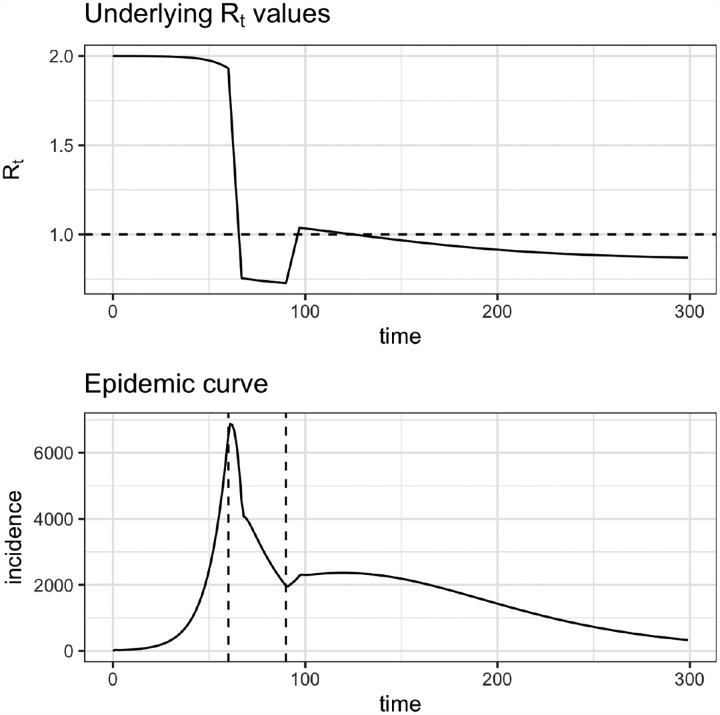
A synthetic time series of new infections (observed daily at the S → E transition) was input into the R_t estimation methods of Wallinga and Teunis, Cori et al., and Bettencourt and Ribeiro [12–14]. Following the published methods, we also tested the Wallinga and Teunis estimator using a synthetic time series of symptom onset events, extracted daily from the E → I transition. The simulated generation interval followed a gamma distribution with shape 2 and rate $\frac{1}{4}$, which is the sum of exponentially distributed residence times in compartments E and I, each with mean of 4 days [19]. R₀ was set to 2.0 initially, then fell to 0.8 and rose back to 1.15 to simulate the adoption and later the partial lifting of public health interventions. To mimic estimation in real time, we truncated the time series at t = 150, before the end of the epidemic. Estimates from the methods of Wallinga and Teunis and Cori et al. were obtained using the R package EpiEstim [20]. Estimates based on the method of Bettencourt and Ribeiro were obtained by adapting code from [6,21] to the package rstan [22]. We initially assumed all infections were observed, which is consistent with the assumptions of all tested methods. Unless otherwise noted, the smoothing window was set to 1 day (effectively, estimates were not smoothed).

Comparison of common methods

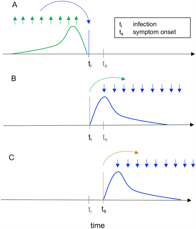
The effective reproductive number at time t can be defined in two ways: as the instantaneous reproductive number or as the case reproductive number [14, 23]. The instantaneous reproductive number measures transmission at a specific point in time, whereas the case reproductive number measures transmission by a specific cohort of individuals (Fig. 1). (A cohort is a group of individuals with the same date of infection or the same date of symptom onset.) The case reproductive number is useful for retrospective analyses of how individuals infected at different time points contributed to spread, and it more easily incorporates data on observed chains of transmission and epidemiologically linked clusters [12,24,25]. The instantaneous reproductive number is useful for estimating the reproductive number on specific dates, either retrospectively or in real time.

Figure 1: Instantaneous reproductive number as estimated by the method of Cori et al. versus cohort reproductive number estimated by Wallinga and Teunis.

For each definition of R_t, arrows show the times at which infectors (upwards) and their infectees (downwards) appear in the data. Curves show the generation interval distribution (A,B), or serial interval distribution (C), conceptually the probability that a given interval of time would separate an infector-infectee pair. (A) The instantaneous reproductive number quantifies the number of new infections incident at a single point in time (t_i, blue arrow), relative to the number of infections incident in the previous generation (green arrows), and their current infectiousness (green curve). The method does not require data beyond time t_i. This figure illustrates the method of Cori et al., which uses data on infection incidence at all times in the previous generation to estimate R_t. The method of Bettencourt and Ribeiro also estimates the instantaneous reproductive number, but instead focuses on the approximate SIR relationship between the number of infections incident at time t_i − 1 and t_i. (B-C) The case reproductive number of Wallinga and Teunis is the average number of new infections that an individual who becomes (B) infected on day t_i (green arrow) or (C) symptomatic on day t_s (yellow arrow) will eventually go on to cause (blue downward arrows show timing of daughter cases). The first definition applies when estimating the case reproductive number using inferred times of infection, and the second applies when using data on times of symptom onset. Because the case reproduction number depends on data from after time t, it is a leading estimator of the instantaneous reproductive number. The magnitude of this lead is less when working with data on times of symptom onset as in (C), because the lag from infection to observation partially offsets the lead (Fig. 2C).

The instantaneous reproductive number is defined as the expected number of secondary infections occurring at time t, divided by the number of infected individuals, and their relative infectiousness at time t [14,23]. It can be calculated exactly within the synthetic data as follows, where β(t) is the time-varying transmission rate, S(t) the fraction of the population that is susceptible, and D the mean duration of infectiousness:

$$R_t^{\text{inst}}=\beta (t)S(t)D.$$ (1)

We assessed the accuracy of all tested methods by comparison to the instantaneous reproductive number (thick black line in Figs. 2, 4, 5 & 6).

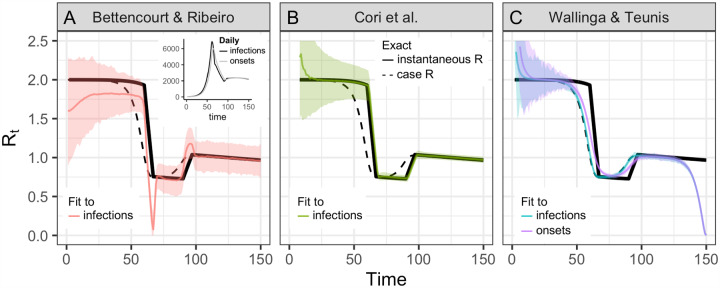
Figure 2: Accuracy of R_t estimation methods given ideal, synthetic data.

Solid black line shows the instantaneous reproductive number, which is estimated by Bettencourt Ribiero and Cori et al. Dashed black line shows the case reproductive number, which is estimated by Wallinga and Teunis. To mimic an epidemic progressing in real time, the time series of infections or symptom onset events up to t = 150 was input into each estimation method (inset). Terminating the time series while R_t is falling or rising produces similar results B.2. (A) By assuming a SIR model (rather than SEIR, the source of the synthetic data), the method of Bettencourt and Ribeiro systematically underestimates R_t when the true value is substantially higher than one. The method is also biased as transmission rates shift. (B) The Cori method accurately measures the instantaneous reproductive number. (C) The Wallinga and Teunis method estimates the cohort reproductive number, which incorporates future changes in transmission rates. Thus, the method produces R_t estimates that lead the instantaneous effective reproductive number and becomes unreliable for real-time estimation at the end of the observed time series without adjustment for right truncation [4,26]. In (A,B) the colored line shows the posterior mean and the shaded region the 95% credible interval. In (C) the colored line shows the maximum likelihood estimate and the shaded region the 95% confidence interval.

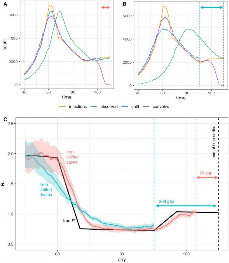
Figure 4: Pitfalls of simple methods to adjust for delays to observation when estimating R_t.

Infections back calculated from (A) observed cases or (B) observed deaths either by shifting the observed curve back in time by the mean observation delay (shift) or by subtracting a random sample from the delay distribution from each individual time of observation (convolve), without adjustment for right truncation. Neither back-calculation strategy accurately recovers peaks or valleys in the true infection curve. The inferred infection curve is less accurate when the variance of the delay distribution is greater (B vs. A). (C) Posterior mean and credible interval of R_t estimates from the Cori et al. method. Inaccuracies in the imputed incidence curves affect R_t estimates, especially when R_t is changing (here R_t was estimated using shifted values from A and B). Finally we note that shifting the observed curves back in time without adjustment for right truncation leads to a gap between the last date in the inferred time series of infection and the last date in the observed data, as shown by the dashed lines and horizontal arrows in A-C.

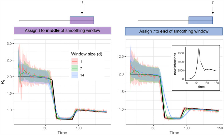
Figure 5:

Accuracy of R_t estimates given smoothing window width and location of t within the smoothing window. Estimates were obtained using synthetic data drawn from the S → E transition of a stochastic SEIR model (inset) as an input to the method of Cori et al. Colored estimates show the posterior mean and 95% credible interval. Black line shows the exact instantaneous R_t calculated from synthetic data.

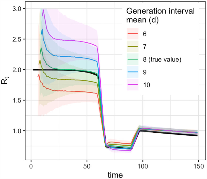
Figure 6:

Biases from misspecification of the mean generation interval (method of Cori et al.).

The methods of Cori et al. [14,15] and methods adapted from Bettencourt and Ribeiro [6,13,21] estimate the instantaneous reproductive number. These approaches were partly developed for near real-time estimation and only use data from before time t (Fig. 1A). Under ideal conditions without observation delays and a window size of one day, neither method is affected by the termination of the synthetic time series at t = 150 (Figs. 2 A&B). These methods are similarly robust if the time series ends while R_t is rapidly falling (Fig. B.2A) or rising (Fig. B.2B). Below we discuss more realistic conditions, in which data at the end of a right-truncated time series would be incomplete due to observation delays.

Of the two methods that estimate the instantaneous reproductive number, the Cori method is more accurate, including in tracking abrupt changes (Fig. 2). An advantage of this method is that it involves minimal parametric assumptions about the epidemic process, and only requires users to specify the generation interval distribution. (The same is true of the Wallinga and Teunis method). Methods adapted from Bettencourt and Ribeiro [13] instead assume a model-dependent form for the relationship between R_t and the epidemic growth rate. The published method is based on the linearized growth rate of an SIR model, and derives an approximate relationship between the number of infections incident at times t and t − 1. Although it is possible to modify the method for more complex models, including SEIR, the SIR-type derivation is most straightforward and is currently used to analyze SARS-CoV-2 spread in real time [6,7, 21]. We found that incorrectly specifying the underlying dynamical model with this method biases inference of R_t, particularly when R_t substantially exceeds one (Fig. 2). When the underlying dynamics of a pathogen are not well understood, this method could lead to incorrect conclusions about R_t. We caution against its use in monitoring the spread of SARS-CoV-2.

The case or cohort reproductive number is the expected number of secondary infections that an individual who becomes infected at time t will eventually cause as they progress through their infection [14,19,23] (Fig. 1B,C). This is the R_t estimated by Wallinga and Teunis. The case reproductive number $R_t^{\text{case}}$ can be calculated exactly at time t within the synthetic data as the convolution of the generation interval distribution w(·) and the instantaneous reproductive number, $R_t^{\text{inst}}$, described in Equation 1 [19],

$$R_t^{\text{case}}={\int }_{u=t}^{\infty }{R}_t^{\text{inst}}w(u-t)du.$$ (2)

We compared the accuracy of each method in estimating the case reproductive number (Fig. 2 and Fig. B.2).

Because the case reproductive number is inherently forward-looking (Fig. 1B,C), near the end of a right-truncated time series it relies on data that have not yet been observed. Extensions of the method can be used to adjust for these missing data and to obtain accurate R_t estimates to the end of a truncated time series [4,26]. But as shown in Fig. 2C, without these adjustments the method will always underestimate R_t at the end of the time series, even in the absence of reporting delays. Mathematically, this underestimation occurs because calculating the case reproductive number involves a weighted sum across transmission events observed after time t. Time points not yet observed become missing terms in the weighted sum. Similarly, infections occurring before the first date in the time series are missing terms in the denominator of the Cori et al. estimator, and so the method of Cori et al. overestimates R_t early in the time series.

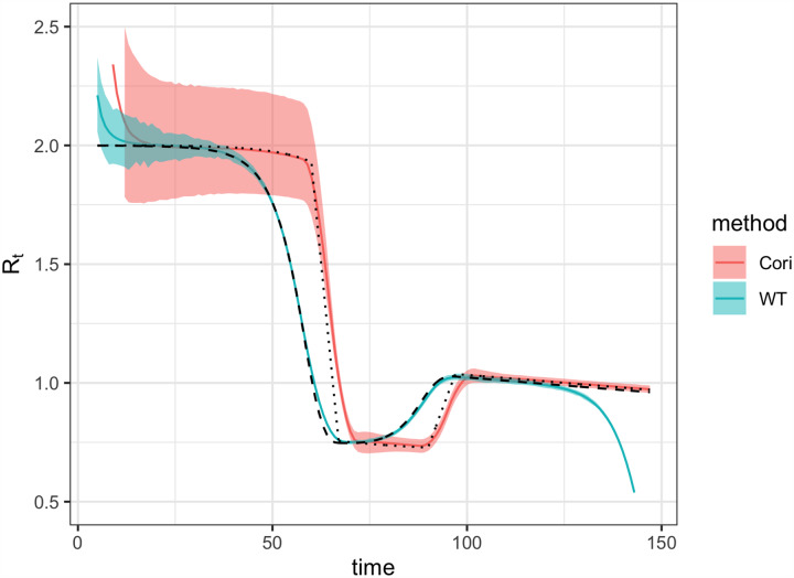
Practically speaking, there are other important differences between the case reproductive number estimated by Wallinga and Teunis and the instantaneous reproductive number estimated by Cori et al. First, the case reproductive number changes more smoothly than the instantaneous reproductive number [23] (Fig. 2B,C). However, if a smoothing window is used, the estimates become more similar in shape and smoothness. Second, the case reproductive number is shifted forward in time relative to the instantaneous reproductive number of Cori et al. (Fig. B). This temporal shift occurs whether or not a smoothing window is used. The case reproductive number produces leading estimates of changes in the instantaneous reproductive number (Fig. 2, B) because it uses data from time points after t, whereas the instantaneous reproductive number uses data from time points before t (Fig. 1). Shifting the case reproductive number back in time by the mean generation interval usually provides a good approximation of the instantaneous reproductive number [2], because the case reproductive number is essentially a convolution of the instantaneous reproductive number and the generation interval (Equation 2) [19]. For real-time analyses aiming to quantify the reproductive number at a particular moment in time, the instantaneous reproductive number will provide more temporally accurate estimates.

Summary

• The Cori method most accurately estimates the instantaneous reproductive number in real time. It uses only past data and minimal parametric assumptions.

• The method of Wallinga and Teunis estimates a slightly different quantity, the case or cohort reproductive number. The case reproductive number is conceptually less appropriate for real-time estimation, but may be useful in retrospective analyses.

• Methods adapted from Bettencourt and Ribeiro [6,13] can lead to biased R_t estimates if the underlying structural assumptions are not met.

Adjusting for delays

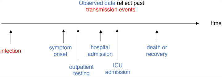
Estimating R_t requires data on the daily number of new infections (i.e., transmission events). Due to lags in the development of detectable viral loads, symptom onset, seeking care, and reporting, these numbers are not readily available. All observations reflect transmission events from some time in the past. In other words, if d is the delay from infection to observation, then observations at time t inform R_t−d, not R_t (Fig. 3). Reconstructing R_t thus requires assumptions about lags from infection to observation. If the distribution of delays can be estimated, then R_t can be estimated in two steps: first inferring the incidence time series from observations and then inputting the inferred time series into an R_t estimation method. Alternatively, a complementary Bayesian approach to infer latent states could potentially estimate the unlagged time series and R_t simultaneously. Such methods are now under development.

Figure 3:

R_t is a measure of transmission at time t. Observations after time t must be adjusted.

Two simple but mathematically incorrect methods for inference of unobserved times of infection have been applied to COVID-19. One method infers each individual’s time of infection by subtracting a sample from the delay distribution from each observation time. This is mathematically equivalent to convolving the observation time series with the reversed delay distribution (Fig. B.1). However, convolution is not the correct inverse operation and adds spurious variance to the imputed incidence curve [27–29]. The delay distribution has the effect of spreading out infections incident on a particular day across many days of observation; subtracting the delay distribution from the already blurred observations spreads them out further. Instead, deconvolution is needed. In direct analogy with image processing, the subtraction operation blurs, whereas the proper deconvolution sharpens (Fig. B.1). An unintended consequence of this blurring is that it can help smooth over weekend effects and other observation noise. But a crucial pitfall is that this blurring also smooths over the main signal of changes in the underlying infection rate: peaks, valleys and changes in slope of the latent time series of infection events. Changes in incidence inform changes in R_t estimates, so while some degree of smoothing may be justified, approaches that blur or oversmooth the inferred incidence time series will prevent or delay detection of changes in R_t, and may bias the inferred magnitude of these changes (Fig. 4C).

The second simple-but-incorrect method to adjust for lags is to subtract the mean of the delay distribution, effectively shifting the observed time series into the past by the mean delay. This does not add variance, and if the mean delay is known accurately, is preferable to subtracting samples from the delay distribution. However, it still does not reverse the blurring effect of the original delay, and it also fails to account for realistic uncertainty in the true mean delay. In practice, the mean delay will not be known exactly and might shift over time.

Reliable methods to reconstruct the incidence time series have not been established for COVID-19, but several directions might be useful. Given a known delay distribution, the unlagged signal could be inferred using maximum-likelihood deconvolution. This method was applied to AIDS cases, which feature long delays from infection to observation [29], and in the reconstruction of incidence from mortality times series for the 2009 H1N1 pandemic [27]. The first method is implemented in the R package backprojNP.

A partial solution to the challenge of adjusting for delays is to rely on observations from closer to the time of infection. Longer and more variable delays to observation worsen inference of the underlying incidence curve. In turn, this makes it more difficult to detect abrupt changes in R_t and to relate changes in R_t to changes in policy. For illustration, when working with synthetic data in which the mean delays to observation are known exactly, the underlying infection curve (Fig. 4A) and underlying R_t values (Fig. 4C) can be recovered with reasonable accuracy by subtracting the mean delay to observation from the observed time series of newly confirmed cases. But because delays from infection to death are more variable, applying the same procedure to observed deaths does not accurately recover the underlying curves of infections or R_t (Fig. 4B,C).

Another advantage of working with observations nearer the time of infection is that they provide more information about recent transmission events and therefore allow R_t to be estimated in closer to real time (Fig. 4C) [28]. Of course, this advantage could be offset by sampling biases and reporting delays. Case data and data on times of symptom onset often vary more in quality than data on deaths or hospital admissions. Users will need to balance data quality with the observation delay when selecting inputs.

Further investigation is needed to determine the best methods for inferring infections from observations if the underlying delay distribution is uncertain. If the delay distribution is severely misspecified, all three approaches (deconvolution, shifting by the mean delay, or convolution) will incorrectly infer the timing of changes in incidence. In this case, methods like deconvolution or shifting by the mean delay might more accurately estimate the magnitude of changes in R_t, but at the cost of spurious precision in the inferred timing of those changes. Ideally, the delay distribution could be inferred jointly with the underlying times of infection or estimated as the sum of the incubation period distribution and the distribution of delays from symptom onset to observation (e.g. from line-list data).

Summary

• Estimating the instantaneous reproduction number requires data on the number of new infections (i.e., transmission events) over time. These inputs must be inferred from observations using assumptions about delays between infection and observation.

• The most accurate way to recover the true incidence curve from lagged observations is to use deconvolution methods, assuming the delay is accurately known [27,29].

• A less accurate but simpler approach is to shift the observed time series by the mean delay to observation. If the delay to observation is not highly variable, and if the mean delay is known exactly, the error introduced by this approach may be tolerable. A key disadvantage is that this approach does not account for uncertainty in the delay.

• Sampling from the delay distribution to impute individual times of infection from times of observation accounts for uncertainty but blurs peaks and valleys in the underlying incidence curve, which in turn compromises the ability to rapidly detect changes in R_t.

Adjusting for right truncation

Near real-time estimation requires not only inferring times of infection from the observed data but also adjusting for missing observations of recent infections. The absence of recent infections is known as “right truncation”. Without adjustment for right truncation, the number of recent infections will appear artificially low because they have not yet been reported [4,26,30–34].

Figure 4 illustrates the consequences of failure to adjust for right truncation when inferring times of infection from observations. Subtracting the mean observation delay m from times of observation (“shift” method in Fig. 4A,B) leaves a gap of m days between the last date in the inferred infection time series and the last date in the observed data. This hampers recent R_t estimation (Fig. 4C). Inferring the underlying times of infection by subtracting samples from the delay distribution (“convolve” method in Fig. 4A,B) dramatically underestimates the number of infections occurring in the last few days of the time series.

Many statistical methods are available to adjust for right truncation in epidemiological data [30–35]. These methods infer the total number of infections, observed and not-yet-observed, at the end of the time series.

In short, accurate near real-time R_t estimation requires both inferring the infection time series from recent observations and adjusting for right truncation. Errors in either step could amplify errors in the other. Joint inference approaches for near real-time R_t estimation, which simultaneously infer times of infection and adjust for right truncation are now in development [35].

Summary

• At the end of a truncated time series some infections will not yet have been observed. Infer the missing data to obtain accurate recent R_t estimates.

Accounting for incomplete observation

The effect of incomplete case observation on R_t estimation depends on the observation process. If the fraction of infections observed is constant over time, R_t point estimates will remain accurate and unbiased despite incomplete observation [12,14]. Data obtained from carefully designed surveillance programs might meet these criteria. But even in this best-case scenario, because the estimation methods reviewed here assume all infections are observed, confidence or credible intervals obtained using these methods will not include uncertainty from incomplete observation. Without these statistical adjustments, practitioners and policy makers should beware false precision in reported R_t estimates.

Sampling biases will also bias R_t estimates [36]. COVID-19 test availability, testing criteria, interest in testing, and even the fraction of deaths reported [37] have all changed over time. If these biases are well understood, it might be possible to adjust for them when estimating R_t. Another solution is to flag R_t estimates as potentially biased in the few weeks following known changes in data collection or reporting. At a minimum, practitioners and policy makers should understand how the data underlying R_t estimates were generated and whether they were collected under a standardized testing protocol.

Summary

• R_t point estimates will remain accurate given imperfect observation of cases if the fraction of cases observed is time-independent and representative of a defined population. But even in this best-case scenario, confidence or credible intervals will not accurately measure uncertainty from imperfect observation.

• Changes over time in the type or fraction of infections observed can bias R_t estimates. Structured surveillance with fixed testing protocols can reduce or eliminate this problem.

Smoothing windows

R_t might appear to fluctuate if cases are severely undersampled and confidence intervals are not calculated accurately. The Cori method incorporates a sliding window to smooth noisy estimates of R_t. Larger windows effectively increase sample size by drawing information from multiple time points, but temporal smoothing blurs changes in R_t and may cause R_t estimates to lead or lag the true value (Fig. 5). Although the sliding window increases statistical power to infer R_t, it does not by itself accurately calculate confidence intervals. Thus, underfitting and overfitting are possible.

The risk of overfitting in the Cori method is determined by the length of the time window that is chosen. In other words, there is a trade-off in window length between picking up noise with very short windows and over-smoothing with very long ones. To avoid this, one can choose the window size based on short-term predictive accuracy, for example using leave-future-out validation to minimize the one-step-ahead log score [38]. Proper scoring rules such as the Ranked Probability Score can be used in the same way, and a time-varying window size can be chosen adaptively [35].

In addition to window size, the position of focal time point t within the window can affect lags in R_t estimates. Cori et al. [14] recommend using a smoothing window that ends at time t. This allows estimation of R_t up to the last date in the inferred time series of infections, but such estimates lag the true value if R_t is changing (Fig 5, right). Because the method assumes R_t is constant within the window, more accurate R_t estimates are obtainable using a smoothing window with midpoint at t (Fig 5, left). The disadvantage of assigning t to the window’s midpoint is that R_t estimates are not obtainable for the last w/2 time units in the inferred infection time series, where w is the width of the window. This impedes near-real time estimation. Thus, for SARS-CoV-2 and other pathogens with short timescales of infection, near real-time R_t estimation requires enough daily counts to permit a small window (e.g., a few days).

Summary

• If R_t appears to vary abruptly due to underreporting, a wide smoothing window can help resolve R_t. However, wider windows can also lead to lagged or inaccurate R_t estimates.

• If a wide smoothing window is needed, consider reporting R_t for t corresponding to the middle of the window.

• To avoid overfitting, choose a smoothing window based on short-term predictive accuracy [38] or use an adaptive window [35].

Specifying the generation interval

R_t estimates are sensitive to the assumed distribution of the generation interval, the time between infection in a primary infection (infector) and a secondary infection (infectee). The serial interval, the time between symptom onset in an infector-infectee pair, is more easily observed and often used to approximate the generation interval, but direct substitution of the serial interval for the generation interval can bias estimated R_t [24,39], especially given the possibility of negative serial intervals [24] (Appendix A). Users must specify the generation interval or estimate it jointly with R_t.

Small misspecification of the generation interval can substantially bias the estimated R_t (Fig. 6). If the mean of the generation interval is set too high, R_t values will typically be further from 1 than the true value—too high when R_t > 1 and too low when R_t < 1. If the mean is set too low, R_t values will typically be closer to 1 than the true value. These biases are relatively small when R_t is near 1 but increase as R_t takes substantially higher or lower values (Fig. 6). Accounting for uncertainty in the generation interval distribution by specifying the variance of the mean (an option when using the adaptation of [6] of methods from Bettencourt and Ribeiro [13]) or resampling over a range of plausible means (an option in EpiEstim [20]) affects the width of the 95% interval but does not correct bias in the mean R_t estimate. A further issue is that the serial interval may decrease over time, especially if pandemic control measures like contact tracing and case isolation are effective at preventing transmission events late in the course of infectiousness [39,40]. Joint estimation of both R_t and the generation interval is possible, depending on data quality and magnitude of R_t [41, 42]. The EpiEstim [15, 20] package provides an off-the-shelf option for joint estimation of the generation interval and R_t.

Summary

• Carefully estimate the generation interval or investigate the sensitivity of R_t to uncertainty in its estimation.

Conclusion

We tested the accuracy of several methods for R_t estimation in near real-time and recommend the methods of Cori et al. [14], which are currently implemented in the R package EpiEstim [20]. The Cori et al. method estimates the instantaneous, not the case reproductive number, and is conceptually appropriate for near real-time estimation. The method uses minimal parametric assumptions about the underlying epidemic process and can accurately estimate abrupt changes in the instantaneous reproductive number using ideal, synthetic data.

Most epidemiological data are not ideal, and statistical adjustments are needed to obtain accurate and timely R_t estimates. First, considerable pre-processing is needed to infer the underlying time series of infections (i.e. transmission events) from delayed observations and to adjust for right truncation. Best practices for this inference are still under investigation, especially if the delay distribution is uncertain. The smoothing window must also be chosen carefully, or adaptively; daily case counts must be sufficiently high for changes in R_t to be resolved on short timescales; and the generation interval distribution must be specified accurately or estimated. Finally, to avoid false precision in R_t, uncertainty arising from delays to observation, from adjustment for right truncation, and from imperfect observation must be propagated. The functions provided in the EpiEstim package quantify uncertainty arising from the R_t estimation model but currently not from uncertainty arising from imperfect observation or delays.

Work is ongoing to determine how best to infer infections from observations and to account for all relevant forms of uncertainty when estimating R_t. Some useful extensions of the methods provided in EpiEstim have already been implemented in the R package EpiNow [35,43], and further updates to this package are planned as new best practices become established.

But even the most powerful inferential methods, extant and proposed, will fail to estimate R_t accurately if changes in sampling are not known and accounted for. If testing shifts from more to less infected subpopulations, or if test availability shifts over time, the resulting changes in case numbers will be ascribed to changes in R_t. Thus, structured surveillance also belongs at the foundation of accurate R_t estimation. This is an urgent problem for near real-time estimation of R_t for COVID-19, as case counts in many regions derive from clinical testing outside any formal surveillance program. Deaths, which are more reliably sampled, are lagged by 2–3 weeks. The establishment of sentinel populations (e.g., outpatient visits with recent symptom onset) for R_t estimation could thus help rapidly identify the effectiveness of different interventions and recent trends in transmission.

Appendix

A. Generation versus serial interval

The generation interval and the serial interval represent two conceptually different quantities. The serial interval is defined as the time between symptom onset in an infector-infectee pair. The generation interval is defined as the time between infection in an infector-infectee pair. Because infected individuals’ times of symptom onset are observable, whereas their times of infection are not, the serial interval is often used as a proxy for the generation interval. As a result of the similarity between the two concepts, and the difficulty of measuring the generation interval empirically, the two are often conflated, obscuring their relevance to different methods for R_t estimation.

As described in [44], the serial interval distribution and the distribution of generation times have the same mean, but they can have different variances, with the variance of the serial interval typically being greater than that of the generation interval [24]. Practically speaking, overestimating the variance of the generation interval may bias R_t estimates [24,39,45]. Moreover, the generation interval is always positive, but the serial interval can be negative in cases where infectiousness occurs before symptom onset. Negative serial intervals have been observed for COVID-19 [46–49]. Failure to account for these negative serial intervals may lead to overestimation of the generation interval, and bias in R_t estimates [24].

The method of Cori et al. defines R_t such that the rate at which an individual infected at time t − s causes secondary infections at time t is given by R_tw_s, where w_s is the infectiousness profile, a probability distribution representing the infectiousness of an individual s days after they have been infected. Biologically, the infectiousness profile depends on the rate at which a given individual is shedding virus. Mathematically, the infectiousness profile represents the probability that person A, the index case, infects person B, a daughter case, exactly s days after person A became infected. This is a generation interval-the probability that s days separates the birth of infection A (the parent) and infection B (the daughter). However, because the distribution of generation times is not observed, the method of Cori et al. suggests using the serial interval distribution as a proxy for the distribution of generation times, and thus often refers to the input to their model as the serial interval distribution. In practice, the serial interval distribution, or the best available approximation thereof, is typically used as the input to the Cori method.

In the published text, Wallinga and Teunis [12] describe the method in terms of symptom onset. Under this convention, the quantity being estimated must be interpreted biologically as the expected number of new infections that a single infected individual who became symptomatic at time t will eventually cause, and the estimation is based on the serial interval, not the generation interval. An alternate, but equally valid convention is to focus on the time of infection, rather than the time of symptom onset. Under this convention, R_t is defined as the number of new infections that an individual infected at time t will eventually cause, and the estimation is based on the generation interval. Here for illustration, we tested the method of Wallinga and Teunis with both times of infection and times of symptom onset as the focal point.

In methods adapted from Bettencourt and Ribeiro [13], the mean generation interval, not the generation interval distribution, is the quantity of interest. Bettencourt and Ribeiro [13] derive a relationship between R_t and the exponential growth rate of the incidence curve by assuming an underlying deterministic SIR system. This relationship depends on the mean infectious period γ⁻¹, which in the SIR model is equal to the generation interval. In the implementation of [6,21], estimates of the mean serial interval (not the serial interval distribution) are used as a proxy for the mean generation interval. It is worth noting that, in that implementation, there is a Bayesian prior distribution on γ, the inverse of the mean “serial interval,” but there is no representation of the distribution of serial intervals across individuals—that distribution is implicitly assumed to be exponential, based on the assumption of SIR-type epidemic structure. That is, the prior distribution represents uncertainty in knowledge about the mean serial interval, not in variability across individuals, which is the main focus of the empirical literature.

B. Appendix figures

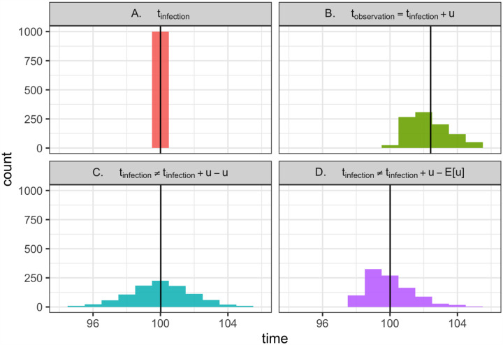
Figure B.1: Why is deconvolution needed to recover latent times of infection?

(A) Consider 1000 individuals, all infected at time 100. (Vertical line shows the mean). (B) Now consider the times at which these individuals are observed. Logically, t_observation = t_infected + u, where u is a random variable describing the delay between infection and observation. Mathematically, this is a convolution of the infection time and the delay distribution. Because u has non-zero variance, observation times are not only shifted into the future but also are blurred across many dates. This blurring is biologically realistic; due to variability in disease progression and care seeking, individuals with the same date of infection will not necessarily be observed at the same time. (C) Using the observations in B, we aim to recover the latent times of infection shown in A. Doing so would require not only shifting into the past but also removing the variance introduced by the observation process, which can be achieved by deconvolution. Instead, as demonstrated here, a common strategy is to subtract u from the times of observation, effectively repeating the convolution shown in B, but this time moving backward in time rather than forward. This is not the correct inverse operation. It fails to remove variance introduced by the observation process (the forward convolution) and adds new, biologically unrealistic variance, further blurring the inferred times of infection. (D) Shifting the times of observation by the mean delay E[u] is also incorrect, as it does not remove the variance from the forward convolution in B. But if the mean delay time is known exactly, this approach is preferable to C, as it avoids adding even more variance. Ultimately, deconvolution methods would be needed to recover A from the observations in B while properly accounting for uncertainty.

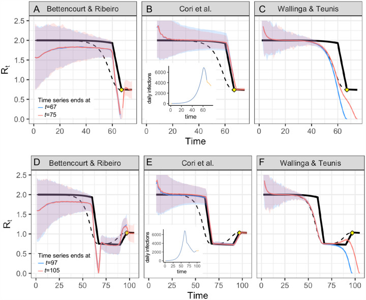
Figure B.2: Real-time accuracy when R_t is rising or falling.

(A-C) Alternate version of Fig. 2 in which the time series ends on the day R_t first hits its minimum value after falling abruptly (time 67, yellow point), or eight days after the changepoint (time 75). (D-F) The time series ends on the day R_t stops rising (time 97, yellow point), or eight days later (time 105). Estimates of the instantaneous reproductive number (A,B,D,E) remain accurate to the end of the time series, and estimates do not change as new observations become available in the 8 days following the changepoint. As in the main text, estimates of the unadjusted case reproductive number (C,F) depend on data from not-yet-observed time points. These estimates become more accurate as new observations are added to the end of the time series (orange vs. blue). Methods to infer the number of not-yet-observed infections can help make estimates of the case reproductive number more accurate in real time [4,26]. All panels show fits to the time series of new infections, and assume all infections are observed instantaneously. Solid black line shows the instantaneous reproductive number, and dashed black line shows the case reproductive number. Colored lines and confidence region show posterior mean and 95% credible interval (A,B,D,E) or maximum likelihood estimate and 95% confidence interval (C,F).

Figure B.3: Smoothed estimates of Cori et al. and Wallinga and Teunis.

Both were estimated using a 7-day smoothing window on a synthetic time series of new infections, observed without delay. The estimates of Cori et al. and Wallinga and Teunis are similar in shape when smoothed, but the estimate of Wallinga and Teunis (the case reproductive number) leads that of Cori et al. (the instantaneous reproductive number) by roughly 8 days, or the mean generation interval. Solid colored lines and confidence regions show the posterior mean and 95% credible interval (Cori et al.) or maximum likelihood estimate and 95% confidence interval (Wallinga and Teunis). Dotted and dashed lines show the exact instantaneous reproductive number and case reproductive number, respectively.

Figure B.4: Synthetic data from SEIR model.

(A) R₀ values were specified as model inputs. The product of R₀(t)S(t) gives the true R_t value. Dashed line shows R_t = 1. (B) Infections observed at the S → E transition. Dashed lines show times at which hypothetical interventions were adopted and lifted.

References

- [1].Pan A, Liu L, Wang C, Guo H, Hao X, Wang Q, et al. Association of Public Health Interventions With the Epidemiology of the COVID-19 Outbreak in Wuhan, China. JAMA. 2020;. doi: 10.1001/jama.2020.6130 [DOI] [PMC free article] [PubMed] [Google Scholar]
- [2].Sciré J, Nadeau SA, Vaughan TG, Gavin B, Fuchs S, Sommer J, et al. Reproductive number of the COVID-19 epidemic in Switzerland with a focus on the Cantons of Basel-Stadt and Basel-Landschaft. Swiss Medical Weekly. 2020;. [DOI] [PubMed] [Google Scholar]
- [3].Kucharski AJ, Russell TW, Diamond C, Liu Y, Edmunds J, Funk S, et al. Early dynamics of transmission and control of COVID-19: a mathematical modelling study. The lancet infectious diseases. 2020;. [DOI] [PMC free article] [PubMed] [Google Scholar]
- [4].Cauchemez S, Boëlle PY, Donnelly CA, Ferguson NM, Guy T, Leung GM, et al. Real-time Estimates in Early Detection of SARS. Emerging Infectious Diseases. 2006;. doi: 10.3201/eid1201.050593 [DOI] [PMC free article] [PubMed] [Google Scholar]
- [5].Flaxman S, Mishra S, Gandy A, et al. Estimating the number of infections and the impact of non-pharmaceutical interventions on COVID-19 in 11 European countries. Imperial College; London; 2020. Available from: 10.25561/77731 [DOI] [Google Scholar]
- [6].rt.live. Available from: http://rt.live [cited 3-June-2020.].
- [7].covidactnow. Available from: https://covidactnow.org/?s=39636 [cited 3-June-2020.].
- [8].Effective reproductive number. Swiss National COVID-19 Science Task Force; Available from: https://ncs-tf.ch/en/situation-report [cited 3-June-2020.]. [Google Scholar]
- [9].Coronavirus disease 2019 Real-time dashboard. School of Public Health, The University of Hong Kong; Available from: https://covid19.sph.hku.hk/ [cited 3-June-2020]. [Google Scholar]
- [10].Modeling Covid-19. Available from: https://modelingcovid.com/ [cited 3-June-2020].
- [11].Lipsitch M, Joshi K, Cobey SE. Comment on Pan A, Liu L, Wang C, et al. Association of Public Health Interventions With the Epidemiology of the COVID-19 Outbreak in Wuhan, China. JAMA. 2020;. doi: 10.1001/jama.2020.6130 [DOI] [PMC free article] [PubMed] [Google Scholar]
- [12].Wallinga J, Teunis P. Different Epidemic Curves for Severe Acute Respiratory Syndrome Reveal Similar Impacts of Control Measures. American Journal of Epidemiology. 2004;. doi: 10.1093/aje/kwh255 [DOI] [PMC free article] [PubMed] [Google Scholar]
- [13].Bettencourt LMA, Ribeiro RM. Real Time Bayesian Estimation of the Epidemic Potential of Emerging Infectious Diseases. PLoS ONE. 2008;. doi: 10.1371/journal.pone.0002185 [DOI] [PMC free article] [PubMed] [Google Scholar]
- [14].Cori A, Ferguson NM, Fraser C, Cauchemez S. A New Framework and Software to Estimate Time-Varying Reproduction Numbers During Epidemics. American Journal of Epidemiology. 2013;. doi: 10.1093/aje/kwt133 [DOI] [PMC free article] [PubMed] [Google Scholar]
- [15].Thompson RN, Stockwin JE, van Gaalen RD, Polonsky JA, Kamvar ZN, Demarsh PA, et al. Improved inference of time-varying reproduction numbers during infectious disease outbreaks. Epidemics. 2019;. doi: 10.1016/j.epidem.2019.100356 [DOI] [PMC free article] [PubMed] [Google Scholar]
- [16].Dehning J, Zierenberg J, Spitzner FP, Wibral M, Neto JP, Wilczek M, et al. Inferring change points in the spread of COVID-19 reveals the effectiveness of interventions. Science. 2020;. doi: 10.1126/science.abb9789 [DOI] [PMC free article] [PubMed] [Google Scholar]
- [17].Lemaitre JC, Perez-Saez J, Azman AS, Rinaldo A, Fellay J. Assessing the impact of non-pharmaceutical interventions on SARS-CoV-2 transmission in Switzerland. Swiss medical weekly. 2020;. doi: 10.4414/smw.2020.20295 [DOI] [PubMed] [Google Scholar]
- [18].Camacho A, Kucharski AJ, Funk S, Breman J, Piot P, Edmunds WJ. Potential for large outbreaks of Ebola virus disease. Epidemics. 2014;. doi: 10.1016/j.epidem.2014.09.003 [DOI] [PMC free article] [PubMed] [Google Scholar]
- [19].Wallinga J, Lipsitch M. How generation intervals shape the relationship between growth rates and reproductive numbers. Proceedings of the Royal Society B: Biological Sciences. 2007;. [DOI] [PMC free article] [PubMed] [Google Scholar]
- [20].Cori A. EpiEstim: Estimate Time Varying Reproduction Numbers from Epidemic Curves.
- [21].Systrom K. The Metric We Need to Manage COVID-19. Available from: http://systrom.com/blog/the-metric-we-need-to-manage-covid-19/ [cited 3-June-2020].
- [22].Stan Development Team. RStan: the R interface to Stan Available from: http://mc-stan.org/.
- [23].Fraser C. Estimating Individual and Household Reproduction Numbers in an Emerging Epidemic. PLoS ONE. 2007;. doi: 10.1371/journal.pone.0000758 [DOI] [PMC free article] [PubMed] [Google Scholar]
- [24].Ganyani T, Kremer C, Chen D, Torneri A, Faes C, Wallinga J, et al. Estimating the generation interval for coronavirus disease (COVID-19) based on symptom onset data, March 2020. Eurosurveillance. 2020;. doi: 10.2807/1560-7917.ES.2020.25.17.2000257 [DOI] [PMC free article] [PubMed] [Google Scholar]
- [25].Hens N, Calatayud L, Kurkela S, Tamme T, Wallinga J. Robust reconstruction and analysis of outbreak data: influenza A(H1N1)v transmission in a school-based population. American journal of epidemiology. 2012;. doi: 10.1093/aje/kws006 [DOI] [PubMed] [Google Scholar]
- [26].Cauchemez S, Boëlle PY, Thomas G, Valleron AJ. Estimating in Real Time the Efficacy of Measures to Control Emerging Communicable Diseases. American Journal of Epidemiology. 2006;. doi: 10.1093/aje/kwj274 [DOI] [PubMed] [Google Scholar]
- [27].Goldstein E, Dushoff J, Ma J, Plotkin JB, Earn DJD, Lipsitch M. Reconstructing influenza incidence by deconvolution of daily mortality time series. Proceedings of the National Academy of Sciences of the United States of America. 2009;. doi: 10.1073/pnas.0902958106 [DOI] [PMC free article] [PubMed] [Google Scholar]
- [28].wyler d, petermann m. A pitfall in estimating the effective reproductive number Rt for COVID-19. medRxiv. 2020;. doi: 10.1101/2020.05.12.20099366 [DOI] [PubMed] [Google Scholar]
- [29].Becker NG, Watson LF, Carlin JB. A method of non-parametric back-projection and its application to AIDS data. Statistics in Medicine. 1991;. doi: 10.1002/sim.4780101005 [DOI] [PubMed] [Google Scholar]
- [30].Lawless JF. Adjustments for reporting delays and the prediction of occurred but not reported events. Canadian Journal of Statistics. 1994;. doi: 10.2307/3315826.n1 [DOI] [Google Scholar]
- [31].McGough SF, Johansson MA, Lipsitch M, Menzies NA. Nowcasting by Bayesian Smoothing: A flexible, generalizable model for real-time epidemic tracking. PLOS Computational Biology. 2020;. doi: 10.1371/journal.pcbi.1007735 [DOI] [PMC free article] [PubMed] [Google Scholar]
- [32].Kalbfleisch JD, Lawless JF. Inference Based on Retrospective Ascertainment: An Analysis of the Data on Transfusion-Related AIDS. Journal of the American Statistical Association. 1989;. doi: 10.1080/01621459.1989.10478780 [DOI] [Google Scholar]
- [33].Höhle M, Heiden Mad. Bayesian nowcasting during the STEC O104:H4 outbreak in Germany, 2011. Biometrics. 2014;. doi: 10.1111/biom.12194 [DOI] [PubMed] [Google Scholar]
- [34].Jvd Kassteele, Eilers PHC, Wallinga J. Nowcasting the Number of New Symptomatic Cases During Infectious Disease Outbreaks Using Constrained P-spline Smoothing. Epidemiology. 2019;. doi: 10.1097/ede.0000000000001050 [DOI] [PMC free article] [PubMed] [Google Scholar]
- [35].Abbott S, Hellewell J, Thompson R, Sherratt K, Gibbs H, Bosse N, et al. Estimating the time-varying reproduction number of SARS-CoV-2 using national and subnational case counts [version 1; peer review: awaiting peer review]. Wellcome Open Research. 2020;. doi: 10.12688/wellcomeopenres.16006.1 [DOI] [Google Scholar]
- [36].Pitzer VE, Chitwood M, Havumaki J, Menzies NA, Perniciaro S, Warren JL, et al. The impact of changes in diagnostic testing practices on estimates of COVID-19 transmission in the United States. medRxiv. 2020;. doi: 10.1101/2020.04.20.20073338 [DOI] [PMC free article] [PubMed] [Google Scholar]
- [37].Weinberger D, Cohen T, Crawford F, Mostashari F, Olson D, Pitzer VE, et al. Estimating the early death toll of COVID-19 in the United States. medRxiv. 2020;. doi: 10.1101/2020.04.15.20066431 [DOI] [Google Scholar]
- [38].Parag K, Donnelly C. Optimising Renewal Models for Real-Time Epidemic Prediction and Estimation. bioRxiv. 2019;. doi: 10.1101/835181 [DOI] [Google Scholar]
- [39].Park SW, Sun K, Champredon D, Li M, Bolker BM, Earn DJD, et al. Cohort-based approach to understanding the roles of generation and serial intervals in shaping epidemiological dynamics. medRxiv. 2020;. doi: 10.1101/2020.06.04.20122713 [DOI] [Google Scholar]
- [40].Lipsitch M, Cohen T, Cooper B, Robins JM, Ma S, James L, et al. Transmission dynamics and control of severe acute respiratory syndrome. Science. 2003;. [DOI] [PMC free article] [PubMed] [Google Scholar]
- [41].Moser CB, Gupta M, Archer BN, White LF. The impact of prior information on estimates of disease transmissibility using Bayesian tools. PloS one. 2015;. [DOI] [PMC free article] [PubMed] [Google Scholar]
- [42].White LF, Wallinga J, Finelli L, Reed C, Riley S, Lipsitch M, et al. Estimation of the reproductive number and the serial interval in early phase of the 2009 influenza A/H1N1 pandemic in the USA. Influenza and other respiratory viruses. 2009;. doi: 10.1111/j.1750-2659.2009.00106.x [DOI] [PMC free article] [PubMed] [Google Scholar]
- [43].Abbott Sam, Hellewell J, Munday J, Thompson R, Funk S. EpiNow: Estimate Realtime Case Counts and Time-varying Epidemiological Parameters Available from: https://github.com/epiforecasts/EpiNow.
- [44].Britton T, Scalia Tomba G. Estimation in emerging epidemics: biases and remedies. Journal of The Royal Society Interface. 2019;. doi: 10.1098/rsif.2018.0670 [DOI] [PMC free article] [PubMed] [Google Scholar]
- [45].Wallinga J, Lipsitch M. How generation intervals shape the relationship between growth rates and reproductive numbers. Proceedings of the Royal Society B: Biological Sciences. 2006;. doi: 10.1098/rspb.2006.3754 [DOI] [PMC free article] [PubMed] [Google Scholar]
- [46].He X, Lau EHY, Wu P, Deng X, Wang J, Hao X, et al. Temporal dynamics in viral shedding and transmissibility of COVID-19. Nature Medicine. 2020;. doi: 10.1038/s41591-020-0869-5 [DOI] [PubMed] [Google Scholar]
- [47].Du Z, Xu X, Wu Y, Wang L, Cowling BJ, Meyers LA. Serial Interval of COVID-19 among Publicly Reported Confirmed Cases. Emerging infectious diseases. 2020;. doi: 10.3201/eid2606.200357 [DOI] [PMC free article] [PubMed] [Google Scholar]
- [48].Nishiura H, Linton NM, Akhmetzhanov AR. Serial interval of novel coronavirus (COVID-19) infections. International Journal of Infectious Diseases. 2020;. doi: 10.1016/j.ijid.2020.02.060 [DOI] [PMC free article] [PubMed] [Google Scholar]
- [49].Tindale L, Coombe M, Stockdale JE, Garlock E, Lau WYV, Saraswat M, et al. Transmission interval estimates suggest pre-symptomatic spread of COVID-19. medRxiv. 2020;. doi: 10.1101/2020.03.03.20029983 [DOI] [Google Scholar]