Fragment pose prediction using non-equilibrium candidate Monte Carlo and molecular dynamics simulations

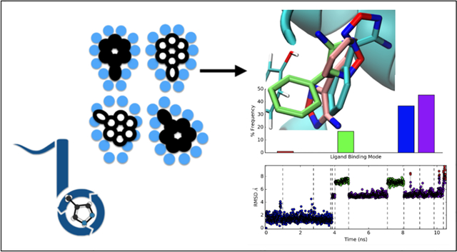
Abstract

Part of early stage drug discovery involves determining how molecules may bind to the target protein. Through understanding where and how molecules bind, chemists can begin to build ideas on how to design improvements to increase binding affinities. In this retrospective study, we compare how computational approaches like docking, molecular dynamics (MD) simulations, and a non-equilibrium candidate Monte Carlo (NCMC) based method (NCMC+MD) perform in predicting binding modes for a set of 12 fragment-like molecules which bind to soluble epoxide hydrolase. We evaluate each method’s effectiveness in identifying the dominant binding mode and finding additional binding modes (if any). Then, we compare our predicted binding modes to experimentally obtained X-ray crystal structures. We dock each of the 12 small molecules into the apo-protein crystal structure and then run simulations up to 1 microsecond each. Small and fragment-like molecules likely have smaller energy barriers separating different binding modes by virtue of relatively fewer and weaker interactions relative to drug-like molecules, and thus likely undergo more rapid binding mode transitions. We expect, thus, to see more rapid transitions between binding modes in our study.

Following this, we build Markov State Models (MSM) to define our stable ligand binding modes. We investigate if adequate sampling of ligand binding modes and transitions between them can occur at the microsecond timescale using traditional MD or a hybrid NCMC+MD simulation approach. Our findings suggest that even with small fragment-like molecules, we fail to sample all the crystallographic binding modes using microsecond MD simulations, but using NCMC+MD we have better success in sampling the crystal structure while obtaining the correct populations.

Graphical Abstract

Introduction

High-throughput screening (HTS) is commonly used in early stage drug discovery to identify potential binders or hits. HTS involves taking a large library of molecules and screening them against a target (e.g. a protein). Hit rates in HTS campaigns are often low, simply due to how vast chemical space can be and the complexity of therapeutic targets.¹ One common strategy in fragment-based drug discovery (FBDD) projects is to conduct the screen using smaller molecules (fragments) to cover a larger portion in chemical space which may lead to higher hit rates. Often in this approach hits tend to be weak binders, but they can serve as a starting point for building a potential lead molecule.² From the pool of hits, medicinal chemists may find a desirable starting scaffold or they can build up new molecules by connecting fragments together in hopes to improve binding affinity. While doing this optimization, chemists must gain an understanding of where and how their molecule binds to their target protein to guide their efforts to optimize the compound’s binding or selectivity.

Some experimental approaches to gaining structural insight on ligand binding include X-ray crystallography, nuclear magnetic resonance (NMR), and surface plasmon resonance (SPR). Each of these approaches present its own set of benefits and challenges but most are costly, time-consuming and difficult.^3,4 For example, X-ray crystallography provides structural information with near atomic-resolution, but obtaining high resolution crystal can be extremely challenging. Especially with FBDD, resolving the binding mode(s) for small molecules and fragments proves challenging as fragments often bind in several different configurations. This often produces X-ray structures which have ambiguous densities around the bound ligand or are generally in too low resolution to definitively resolve the fragment binding mode(s).⁵

Here, with these ambiguous densities in the crystal structures, computational approaches may aid in the design process by resolving ambiguities through predicting fragment binding modes. Computational methods like docking or molecular dynamics (MD) simulations are some common approaches used in helping to determine fragment binding modes.^6–8 If these techniques are accurate enough, computational chemists can apply them to make sense of partial occupancy data and help rescue structure-based design work on fragments that might otherwise have stalled.

Docking is a computationally inexpensive technique which generates a variety of configurations or poses by placing the ligand into a static structure of the apo-protein and subsequently scoring each generated candidate. It can be performed at high speeds by neglecting conformational changes in proteins which might normally occur on binding. This often results in sacrificing accuracy–making it difficult to distinguish binders from non-binders.^9–13 Of course, there are also flexible docking approaches but these usually neglect protein strain and typically do not demonstrate dramatically better performances.¹⁴ Instead, docking can often be used to understand the conformational space of the ligand and provide some initial insight on how a ligand may fit in the binding site. Several studies have shown that docking does not reliably find experimental binding modes of ligands.^13,15 In view of these limitations, here, we use docking to generate a variety of configurations to hopefully provide coverage of the entire binding site and all reasonable binding mode possibilities, and use these as starting points for our simulations.

Unlike docking, MD simulations resolve—in full atomistic detail—the overall dynamics of the protein-ligand system by solving Newton’s equations of motions in discrete timesteps.^16,17 This can get very computationally expensive if one wants to simulate biological timescales as MD simulations must take timesteps which are constrained by the fastest motion in the system (e.g. bond vibrations at 1–2 femtoseconds). One may use schemes like hydrogen mass re-partitioning¹⁸ to enable one to take longer timesteps (e.g. 4fs) by slowing down hydrogen bond stretching, but interesting biological motions occur at much larger timescales necessitating large numbers of timesteps and great computational cost. Interesting biological motions like protein folding or other large conformational changes have timescales ranges from 10⁻⁶s (μs) to 10⁰s or even longer,¹⁹ requiring extremely long compute times if one aims to capture these types of motions.

Fortunately, recent advancements in technology, like the introduction of computing using graphics processing units (GPUs), have made achieving microsecond (or even millisecond) long MD simulations fairly routine. Still, despite using longer timesteps and newer technologies, the utility of MD simulations in the drug discovery process has been hindered by MD’s inability to adequately sample the conformational space. Often, MD simulations of a protein-ligand complex will see the ligand remain trapped in the binding mode the simulation had started in and will fail to capture any transition into alternative binding modes.

For FBDD, MD simulations may hold some value given that fragments are small and rigid enough that transitions between binding modes may occur at shorter timescales. In this case, MD simulations could then resolve potential binding modes and reveal important stabilizing protein-ligand contacts–that is, if such contacts form on reasonable timescales (nanoseconds to milliseconds). But in some cases, binding mode transitions may require conformational changes in the protein which may take beyond the millisecond timescale before a transition can even occur.^20,21 Although these challenges in adequate sampling of the biologically relevant timescales remain an issue to this day, recent advancements in the field have resulted in new ways to address sampling challenges which we apply within this study. We note that in this study, we are mostly focused on addressing problems of sampling ligand binding modes that occur in the absence of slow protein conformational degrees of freedom.

One example of an enhanced sampling approach is a hybrid simulation approach which combines non-equilibrium candidate Monte Carlo (NCMC)²² move proposals with traditional MD simulations. We previously implemented this NCMC+MD approach in a software package called BLUES: Binding modes of Ligands Using Enhanced Sampling,²³ which aims to accelerate sampling of ligand binding modes by proposing random rotational moves on the ligand and then runs a conventional MD simulation. BLUES is similar to using traditional Monte Carlo (MC) moves with MD, except that it uses a gradual non-equilibrium based switching protocol while performing perturbations to the ligand instead of an instantaneous perturbation. In theory, this allows us to perform larger perturbations to the ligand and increase acceptance of proposed moves over traditional MC. With the BLUES approach, we hypothesize that we will observe better sampling of ligand binding modes and be able to identify the experimental ligand binding modes over using traditional MD simulations. Previous work using BLUES has shown success in accelerating sampling of ligand binding modes in the simple model systems of toluene and iodotoluene bound to the T4 lysozyme L99A mutant.²³ Here, we are interested in applying BLUES to a more complex target with pharmaceutical relevance to evaluate its utility beyond a simple model system.

In this retrospective study, we are interested in using computational methods to identify binding modes for fragments which bind to a protein called soluble epoxide hydrolase (SEH). SEH has been hypothesized to have therapeutic potential in cardiovascular diseases, inflammatory diseases, and neurological diseases, which has spurred efforts in developing SEH inhibitors. Specifically, SEH is involved in the breakdown of epoxyeicosatrienoic acids (EETs), acids with cardiovascular effects such as vasodilation and anti-inflammatory actions. Through slowing the degradation of EETs (via SEH inhibition), it has been hypothesized to induce neuroprotective, cardioprotective, and anti-inflammatory effects. In vitro studies with murine models found that SEH inhibition significantly lowered blood pressure, bolstering its hypothesized role in blood pressure regulation.^24–26

Here, we apply docking, MD, and (NCMC+MD) BLUES simulations on a small set of 12 fragments which bind to SEH and evaluate their effectiveness in identifying their binding modes. For the remainder of this paper, we define binding modes as experimentally or simulation-determined metastable bound states; ligand poses are defined as the configurations generated from docking. In some cases, MD simulations can successfully distinguish experimental binding modes from decoy poses better than using docking alone.^27,28 Thus, we will investigate if using microsecond MD simulations or our BLUES (NCMC+MD) enhanced sampling approach provide any value, beyond docking, for identifying the SEH fragment binding modes. We will compare poses generated from docking and the metastable binding modes sampled from MD and BLUES against experimentally obtained x-ray crystal structures. Through this study, we aim to provide insight on the value computational methods can provide in identifying the crystallographic binding modes and finding additional binding modes.

Methods

SEH apo-protein preparation

Prior to beginning this study, our OpenEye Scientific collaborators provided the SEH structure, the location of the binding site where ligands would be docked, and a set of 47 ligands in the form of SMILES strings. The initial SEH structure from OpenEye Scientific was missing residues. We found the apo SEH structure in the Protein Data bank (PDBID:5AHX), built in the missing residues with PDBFixer, and used this structure for the remainder of the study.²⁹ The apo SEH structure was altered using the PDB2PQR web server,³⁰ which uses PROPKA2.0 to assign residue protonation states. We protonated residues at pH 8.5 to match experimental conditions, using AMBER parameters^31–33 and we removed crystallographic waters from the system. The PQR file was then converted back to a PDB file with ParmEd (v3.0.1). We aligned the corrected apo SEH structure to the SEH structure provided by OpenEye Scientific to ensure the predefined docking site was the same.

The SEH protein contains 2 domains, a phosphatase domain (N-terminus) and a hydrolase domain (C-terminus) connected by a flexible proline rich linker.³⁴ The predefined docking site was only located in the C-terminal hydrolase domain, so to reduce computational cost, we removed the N-terminal domain from residue 0 to residue 224 (Fig. 1). We analyzed the structural integrity of the truncated protein by averaging the RMSD of the protein backbone over a 1 microsecond MD simulation. The average RMSD of the truncated protein backbone was 2.1 Angstroms suggesting the C-terminus was relatively unaffected by the removal of N-terminus. The slight spikes in RMSD correspond to fluctuations in the flexible linker region and did not affect the overall integrity of the C-terminal hydrolase domain–where the binding site was located. In Figure 3, we show the entire binding site located in the C-terminus domain as defined by our collaborators.

Figure 1:

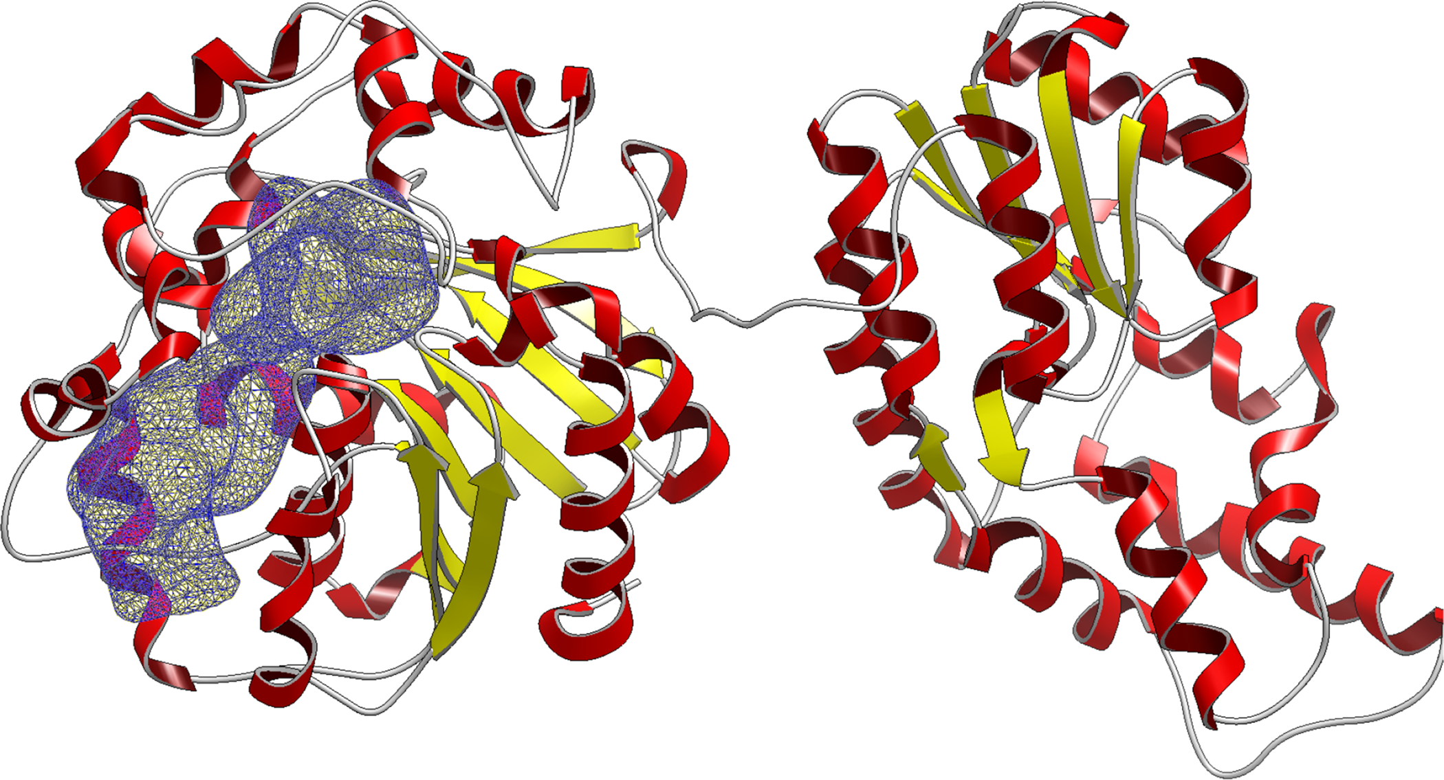
The complete SEH protein structure with the C-terminal domain (left) and the N-terminal domain (right). The docking site is highlighted (blue) in a mesh representation. The N-terminal domain (right) was removed to reduce computational costs, keeping the C-terminal domain with the defined docking site.

Figure 3:

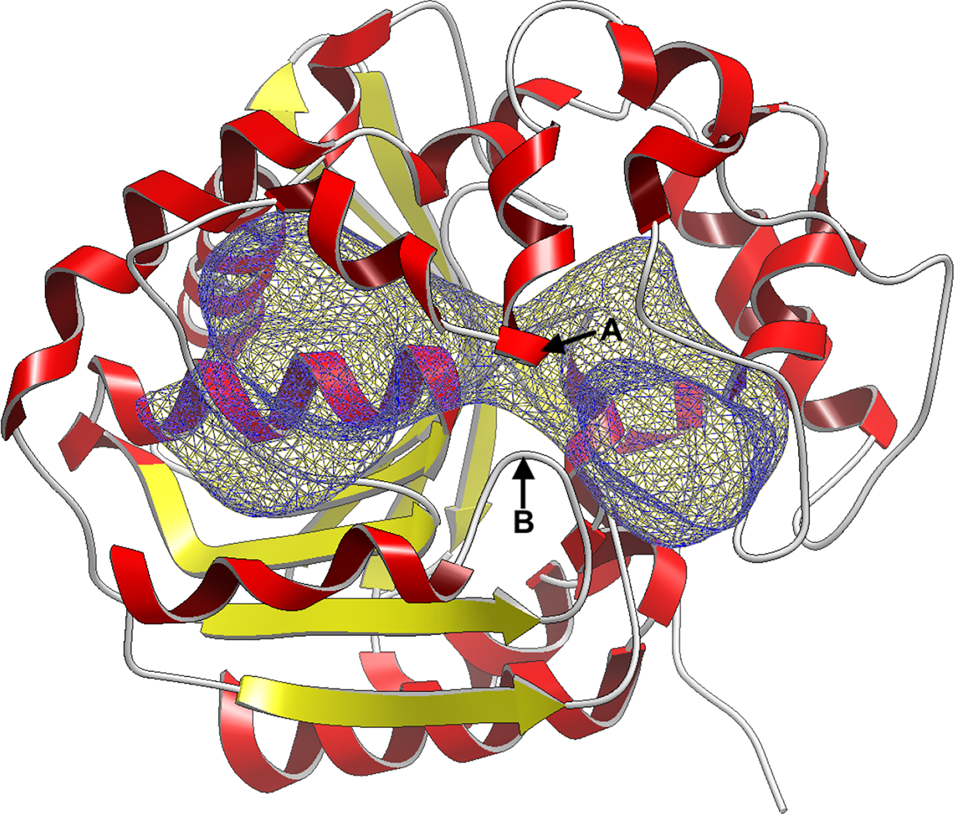
Truncated SEH protein structure (C-domain only) with the the docking site is highlighted (blue) in a mesh representation. We divide the full cavity into two sub-cavities denoted by left and right. The sub-cavity division is best denoted at the two loops marked as A and B in the figure. In the SEH apo protein structure, point A is closest to residue VAL381 and point B is closest to residue VAL499. We treat each sub-cavity separately in our analysis to better resolve binding modes within each sub-cavity.

Here, we define two sub-cavities (left/right) which are separated by two loops which form at residues VAL381 (A) and VAL499 (B), creating a cleft in the center of the SEH binding site (Fig. 3). Throughout this study, we treat the left and right sub-cavity separately as we did not observe transitions between them in our simulations. By performing our analysis on each sub-cavity separately, we are better able to resolve the binding modes and timescales for transitions between binding modes, relative to trying to resolve the transition timescales between the sub-cavities.

Ligand preparation and docking

From a set of 47 ligands given to us by our OpenEye Scientific collaborators, we chose to study a smaller subset of 12 ligands (Fig. 4). The initial set of 47 ligands were taken from a fragment-based drug discovery campaign from AstraZeneca.³⁵ Here, we chose ligands based on the overall size and number of rotatable bonds. Particularly, we were interested in only studying small and rigid fragment molecules as we expected to observe more binding mode transitions during our simulations, due to their size and rigidity. The molecule set ranged from 133.13 to 156.73 ų in shape volume with 0 to 1 rotatable bonds.

Figure 4:

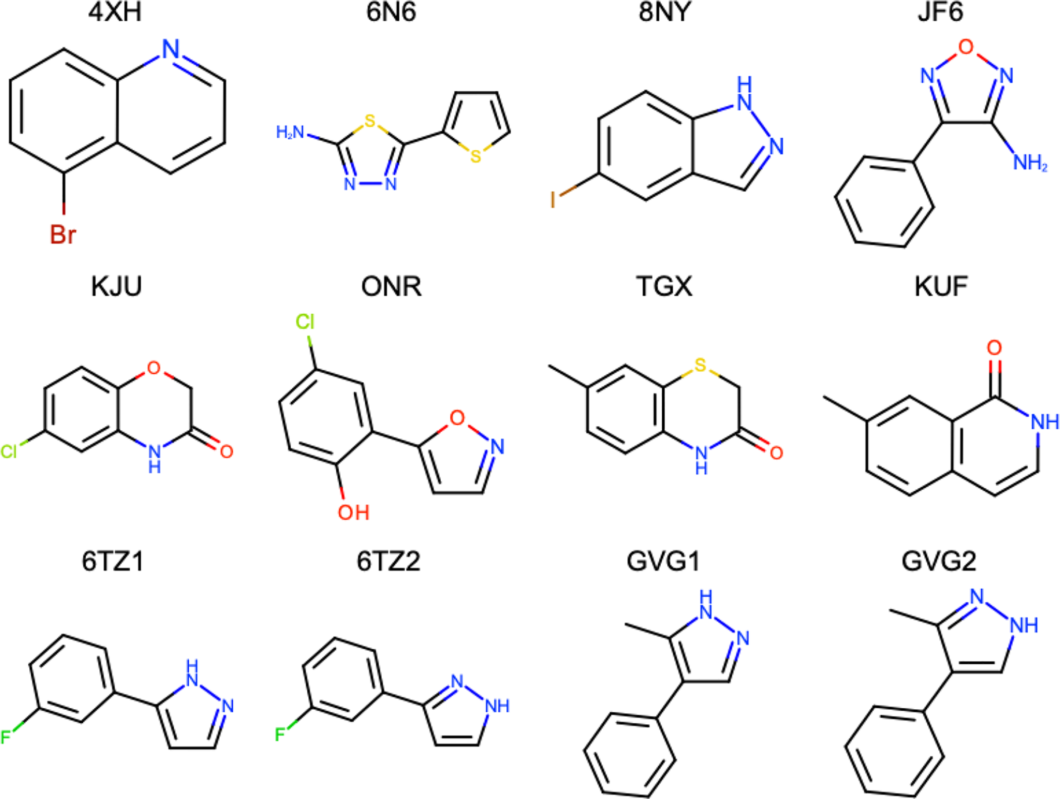
2D representation of molecules used in this study and their identifying label.

We used openmoltools (v0.8.1)³⁶ and OpenEye toolkits³⁷ to convert each ligand SMILES string to a 3D structure and then we assigned charges using the OEAM1BCC charging scheme from the OEQUACPAC library.³⁷ This scheme assigns AM1 Mulliken-type partial charges with bond-charge corrections to the ligand atoms.³⁸ Then, we generated 1000 conformers of each charged ligand using OpenEye’s OMEGA (20180212).³⁹ These conformers were then docked into the SEH apo protein structure using FRED from OEDock(v3.2.0.2), generating 1000 docked poses, and scored with the Chemgauss4 scoring function.⁴⁰

From the 1000 generated docked poses, we wanted to select the most distinct and use them as our starting positions for our simulations. Here, we define distinct docked poses as poses which are dissimilar from one another. Some studies have shown that docking is an unreliable method for identifying the true binding mode using the top scoring pose.¹³ Given this, we believed that the top scoring poses would often be far from the true binding mode and thus, we did not retain them and use them as starting points for our MD simulations to ensure broad coverage of possible binding modes/sites. This was done without utilizing experimental binding modes. In analysis after our calculations, we confirmed that the top scoring docked poses are not generally close to the crystallographic binding modes (Fig. 5).

Figure 5:

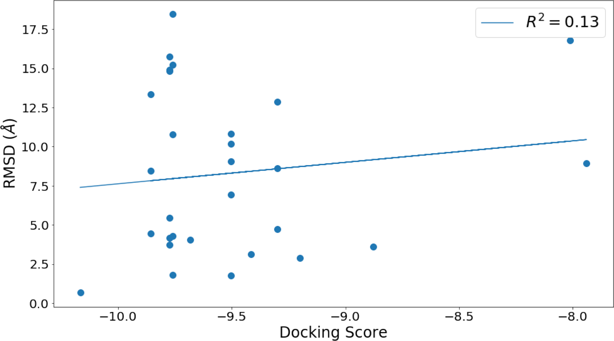
Docking score and the calculated RMSD (Å) to the crystallographic binding modes from the top scoring docked poses.

By selecting the distinct poses generated from docking, we have a variety of starting configurations in our simulations and provide reasonable coverage of the protein binding site. Regardless of the starting positions, given enough simulation time and the fragment-like properties (i.e. small and rigid properties) of the molecules we are simulating, we should see convergence to the true binding mode given the forcefields, protonation states, accuracy of our model, and simulation timescales used in this study. However, how much “enough simulation time” truly is remains an open question in general. We describe the filtering and selection process below.

MDS-RMSD Filtering: Unique pose selection

First, we generate a RMSD-based similarity matrix of the 1000 generated docked poses. That is, we compute the RMSD, using only the ligand heavy atoms, from each docked pose to every other docked pose. This gives us an NxN similarity matrix (N=1000), in which our measure of similarity is based on the calculated RMSD between the docked poses (Fig. 6). Next, we apply a technique called Multi-Dimensional Scaling (MDS) through scikit-learn (v0.19.0)⁴¹ in order to reduce our NxN dimensional space into a 2D space, where we can then apply clustering techniques. MDS is a method which transforms our similarity matrix and projects each object (i.e pose) into a lower dimensional space in such a way that the distance between objects (i.e poses) are preserved as best as possible. In other words, when we project into a 2D space, poses which are similar (low RMSD) will appear closer together and poses which are dissimilar (high RMSD) will appear farther away.

Figure 6:

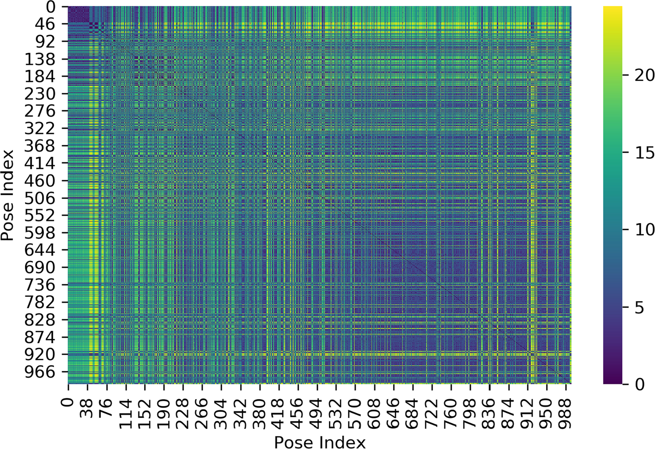
RMSD (Å) similarity matrix from 1000 docked poses for 8NY. Poses which are similar will have a low RMSD represented by darker colors (blue to purple) and poses which are dissimilar will have a high RMSD represented by brighter colors (green to yellow). This shows the raw similarities between docked poses.

After applying MDS to our RMSD similarity matrix, we transform our NxN dimensional space and take our first two MDS components to project the data into a 2D scatter plot. This enables us to easily apply K-means clustering⁴² (from scikit-learn) to group up similar poses and separate dissimilar poses with the first two components which best represent the pair-wise similarity distances. A notable downside to K-means clustering is that one has to specify the number of clusters to be used to separate the data points. To avoid bias, we use silhouette scoring⁴³ (from scikit-learn) to automatically determine the best number of clusters to use to separate our data points. Silhouette scores range from −1 to +1 and evaluates how similar objects belonging to the same cluster are (cohesion) and how dissimilar those objects are with other clusters (separation) (Left: Fig. 7). High values (closer to +1) indicate that the object is similar to other objects within the same cluster and dissimilar to objects in neighboring clusters. Low values (closer to −1) indicate that the object is dissimilar to others within the same clusters and similar to objects in neighboring clusters. A low total silhouette score indicates that the clustering configuration is likely incorrect with either too many or too few clusters, so we can use the total silhouette score as a way to select the optimal number of clusters.

Figure 7:

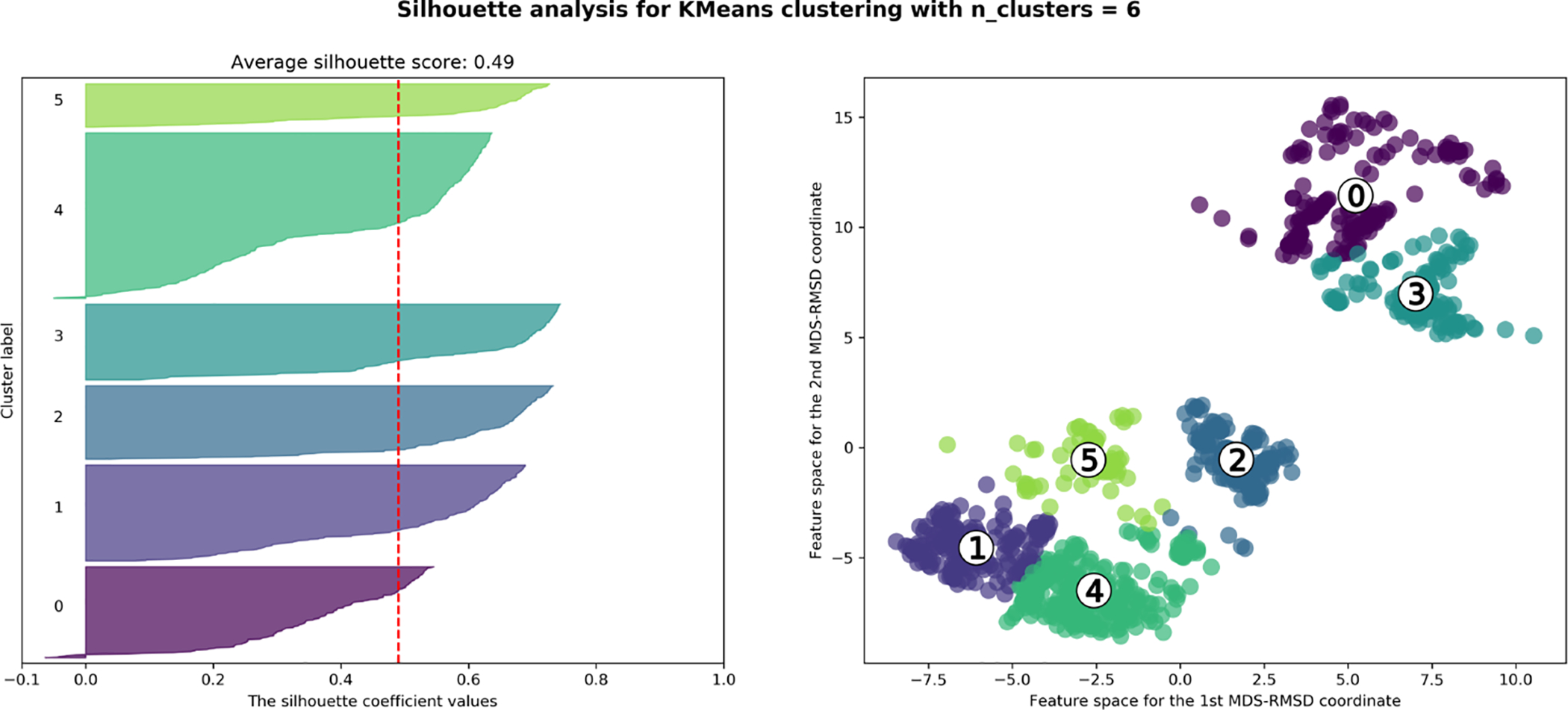
Left: Silhouette scores from 1000 docked poses for 8NY using 6 clusters from K-means clustering. Right:MDS-RMSD scatter plot for 1000 docked poses for 8NY with K-means clustered points using 6 clusters. The cluster centroids are denoted by a number in white circles.

We apply K-means clustering using a range of 2–9 clusters on our MDS-RMSD scatter plot and score each round of clustering using silhouette scores. We selected the number of clusters K maximizing total silhouette score, and then used this to partition our 1000 docked poses in MDS-RMSD space and set the number of starting poses to be used for our simulations. Using the K clusters which maximized the silhouette score, we then selected the pose closest to the calculated centroid of each cluster as the representative pose for starting our simulations (Right: Fig. 7).

Molecular Dynamics and BLUES Simulations

In this study, we used two simulation approaches: traditional molecular dynamics (MD) simulations and our hybrid approach called BLUES: Binding modes of Ligands Using Enhanced Sampling,²³ which combines Non-equilibrium Candidate Monte Carlo (NCMC)²² move proposals with MD. Both MD and BLUES simulations using OpenMM (v7.1.1)⁴⁴ with the same solvated SEH system. For our simulations, the truncated SEH protein (consisting of only the C-terminal domain) was parameterized with amber99sbildn forcefield for the protein and GAFF2 for the ligands, and solvated with TIP3P waters.⁴⁵

We performed a maximum of 30,000 energy minimization steps and a 3 stage (NVT, NPT, NPT) equilibration protocol which we describe as follows. In each equilibration stage, a restraint force is placed on the α-Carbons of the protein backbone and the ligand heavy atoms, where we successively decrease the force from $2.0\frac{\mathit{\text{kcal}}}{\mathit{\text{mol}}\cdot {\AA }^2}$ to $0.5\frac{\mathit{\text{kcal}}}{\mathit{\text{mol}}\cdot {\AA }^2}$ to $0.1\frac{\mathit{\text{kcal}}}{\mathit{\text{mol}}\cdot {\AA }^2}$ at each stage. After equilibration, we ran 1 microsecond (μs) using molecular dynamics (MD) and 600 nanoseconds (ns) to 1 microsecond using BLUES for each pose selected by our MDS-RMSD filtering protocol (described in the previous section). We note that some BLUES simulations were run less than 1 microsecond due to limitations in our available compute resources. Our simulations were run using 4 femtosecond (fs) timesteps and with the hydrogen-mass repartitioning scheme.¹⁸

Briefly, we describe our protocol for BLUES simulations. A BLUES simulation begins with the NCMC phase, which involves proposing a random rotation about the ligand center of mass and then relaxes via a series of non-equilibrium switching steps which alchemically scale the ligand iterations off/on over N steps. This is in contrast to traditional Monte Carlo, which involves performing an instantaneous change to the ligand coordinates. Specifically, interactions are controlled via a parameter (λ_0→1) which scales the ligand interactions with the surrounding environment. Our non-equilibrium switching protocol begins with the fully interacting ligand at λ₀ and then we alchemically scale the ligand forces off until λ_0.5, where the ligand is no longer interacting with surrounding atoms. We perform the proposed random rotation on the non-interacting ligand and then alchemically scale the ligand forces back on until λ₁, where the ligand is fully interacting and in the proposed position. Over the series of N NCMC switching steps, we accumulate the total non-equilibrium work done and use this in acceptance or rejection of the proposed move (following the Metropolis-Hasting acceptance criterion⁴⁶). After the Metropolization step, we follow-up using traditional MD methodology and repeat the cycle (NCMC -> MD -> NCMC…etc.) for I iterations.

Determination of Binding Modes with TICA and PCCA

We divide the SEH binding site (Figure 3) into two sub-cavities denoted as “left” and “right” and analyze simulation data from these two sub-cavities separately, as we rarely observed transitions between them. That is, simulations which started with dock poses in the right sub-cavity were pooled together and vice versa, but simulations in each sub-cavity were kept separate, since very few simulations exhibited transitions and thus pooling data across sub-cavities would have complicated analysis. By treating the two sub-cavities separately, we are better able to distinguish between binding modes sampled within each sub-cavity and understand their timescales, over the timescale to transition between sub-cavities. In other words, we can better distinguish rapid transitions between binding modes within each sub-cavity over the slow transitions between sub-cavities. Additionally, if we had pooled together simulation data from both sub-cavities, our silhouette scores would always suggest 2 binding modes, which is actually just the separation of binding modes between the two cavities.

Using PyEMMA (v2.5.5), we analyzed and built Markov State Models (MSM) separately between our MD and BLUES simulations. MD simulation frames were stored every 25,000 steps (100ps/frame) and BLUES simulation frames were stored every 10,000 steps (40ps/frame). In this study, we apply a method called time-lagged independent component analysis (TICA) with perron-cluster cluster analysis (PCCA) to define our metastable binding modes sampled during our simulation. Here, we analyzed our simulations using the coordinates of the ligand heavy atoms as our chosen feature set. In Figure 8, the appropriate lagtime for TICA was chosen by performing an analysis on the VAMP2 score^47–49 by varying the TICA dimensions parameter for several lag times. VAMP2 score measures the kinetic variance in our chosen feature set and provides a heuristic for selecting an appropriate lagtime to discretize our input coordinates in TICA space. Here, we chose a lag time of 1ns to discretize our MD simulations, but lag times below 1ns would have been an appropriate choices as well. For our BLUES simulations, we chose a lag time of 200ps to discretize the simulation data as this corresponds to the amount of simulation time between each move proposal, where a change in binding mode may occur. We applied TICA⁵⁰ to extract the slow order parameters from our feature set (ligand heavy atom coordinates). From our TICA coordinates, we cluster our simulation frames into discrete microstates using k-means clustering. This gives us a set of N discrete microstates (i.e. simulation frames) which we map into the coordinate space of the first 2 TICA components (Fig. 9), where N is defined as the square root of the total number of simulation frames (the default setting for PyEMMA).

Figure 8:

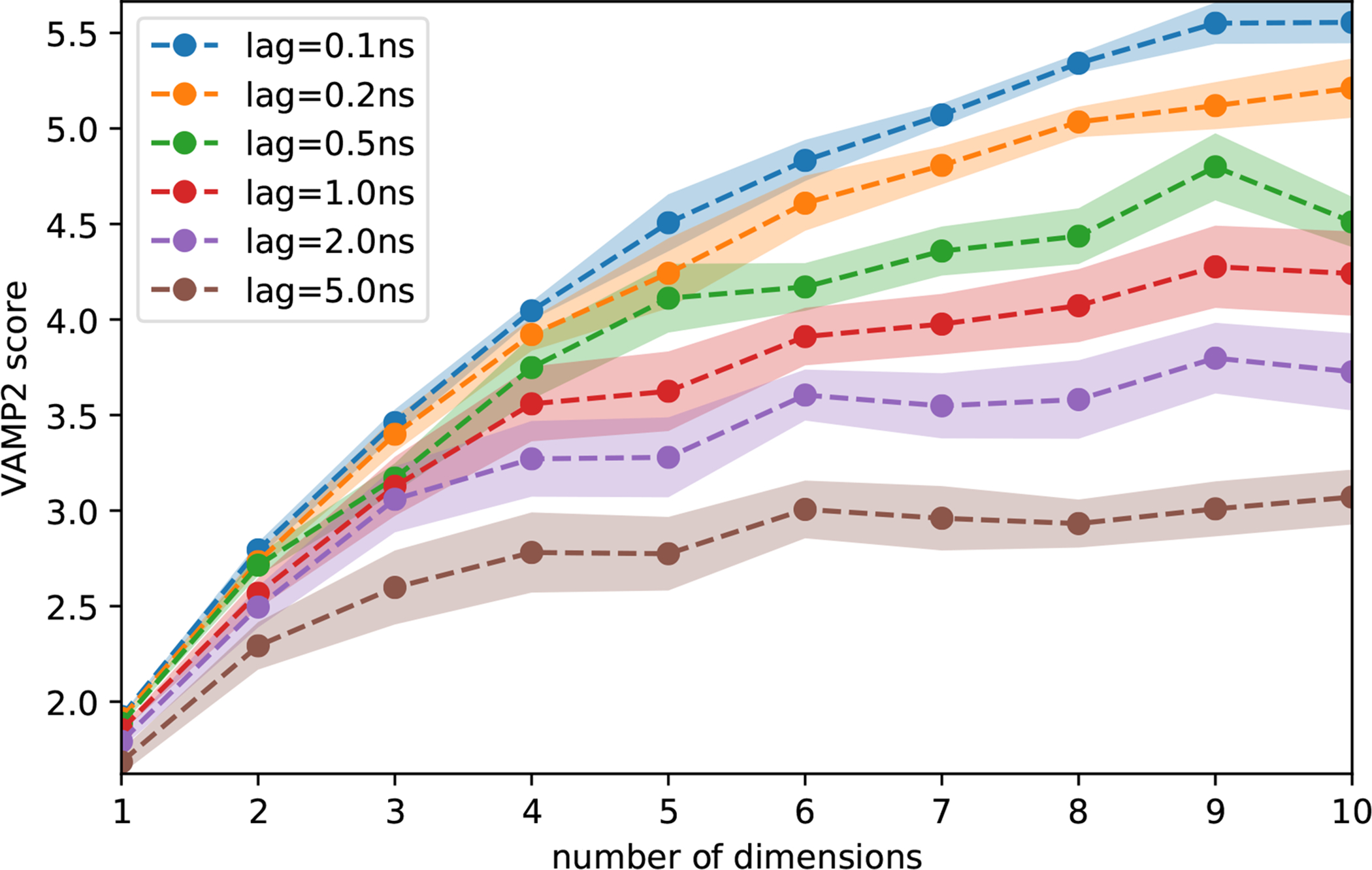
VAMP2 scores analysis for 8NY from our MD simulations. This plots the number of TICA dimensions against the VAMP2 scores for several lag times (nanoseconds). At lag times above 1ns we do not observe as large of an increase in the VAMP2 score when using more than four dimensions, i.e. the first four dimensions contains most of the relevant information of the slow dynamics.

Figure 9:

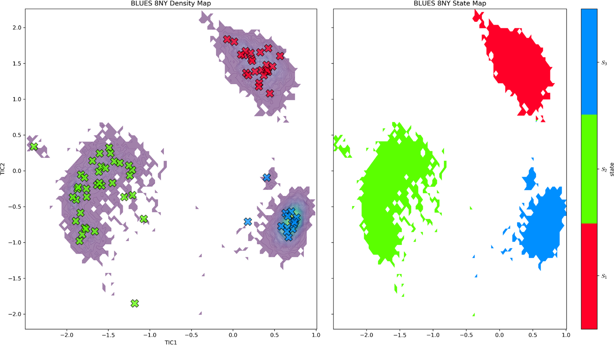
Left: Time-lagged independent component analysis (TICA) plot for binding modes of 8NY located in the right sub-cavity using the first two TICA components from our BLUES simulations. Discrete microstates (i.e. simulation frames are denoted by Xs. Each microstate has been assigned to a macrostate by PCCA which define our metastable binding modes sampled during our simulation. We find 3 states (red, green, blue) or binding modes sampled from simulations of 8NY in the right sub-cavity. Right: Shows the sampling density from our BLUES simulations for the 3 macrostates defined by PCCA, where tighter clusters are suggestive of higher stability for that particular macrostate.

In Figure 9, we define our macrostates or metastable binding modes by assigning each microstate to a given K number of macrostates via PCCA.^51,52 To determine the appropriate number of K macrostates to use, we evaluate the clustering using silhouette scoring⁴² (discussed previously). In our analysis we represent each macrostate by randomly draw 50 simulation frames from the pool of microstates assigned to each of the K macrostates.

In Fig S13, we plot the RMSD of the ligand heavy atoms relative to the crystal structure and color each time point by assigning it to the macrostate which minimizes the RMSD. Specifically, we compute the ligand heavy atom RMSD to the 50 representative microstates (simulation frames) belonging to each macrostate; then, assign it to the macrostate which minimizes the RMSD. We can then compute the populations or amount of simulation time spent within each binding mode by counting how many frames fall within each binding mode (Fig. S12).

Crystal Structure Selection and Refinement

The fragment binding data used in this study was a subset of the 55 complex structures and 1 apo structure with associated affinity data published by L. Öster et al.⁵³ All 55 complex structures were re-refined using phenix.refine (version 1.14.3283)^54,55 with AFITT⁵⁶ generated MMFF94s gradients on the small molecule ligand-complexes used in phenix.refine (PHENIX-AFITT). All refinements using phenix.refine or PHENIX-AFITT used six refinement macrocycles. The resulting structures were aligned to the apo structure (PDBID:5AHX) using defaults options for protein alignment in the OpenEye SpruceTK.⁵⁷ The ten fragment complex structures used for prediction (PDBID:5AI0, 5AI6, 5AIB, 5AIC, 5AK4, 5AKG, 5AKX, 5ALE, 5ALV, 5AM2) were further re-refined in an attempt estimate the occupancy of the fragment in the binding site and to determine if an automated ligand placement algorithm (AFITT)⁵⁸ agreed with the conformation and placement done by L. Öster et al.⁵³ The re-refinement protocol was as follows: 1) remove the ligand and refine using phenix.refine the resulting protein, excipients and solvent; 2) AFITT⁵⁸ was used to automatically fit fragment to the resulting difference density; 3) the new fragment placement was checked to see if significantly different from the deposited placement; 4) the new complex was re-refined using PHENIX-AFITT; and 5) the structure was refined with occupancy refinement of the ligand turned on and automatically generated Translational, Librational, and Screw (TLS) constraints for PHENIX-AFITT. The refinement and occupancy data for all ten structures can be found in supporting data tables S3, S2 and S1. The median root mean square deviation (RMSD) between the deposited and re-refined ligands was 0.11 Å with a maximum of 1.4 Å for 6N6 (PDBID:5AK4).

The ten structures used in this study were initially re-refined using PHENIX-AFITT for two reasons. The first was to generate ligand bond lengths, angles and torsions fit using energetics from a small molecule force field – in this case MMFF94s. The second was to assess whether additional low occupancy conformations or binding modes existed. While the depositors⁵³ were very careful and thorough in fitting the ligands for these structures there is prior evidence, from the recent qFit publication by G. C. P. van Zundert et al.,⁵⁹ that up to 29% of protein-ligand complexes could have ligand heterogeneity or unmodeled alternate binding modes. Our initial analysis suggested some of the ten structures had evidence of alternate binding modes, making them an ideal test cases for a method geared towards sampling of binding modes. We used a method based on AFITT^56,58 but similar in principle to qFit and found three cases of previously unmodeled heterogeneity. They were a missing alternate conformation for TGX, a different binding conformation for 6N6, and an additional binding mode for GVG. For 6N6 the new conformation rotates the thiodiazol-2-amine ring by 180° into an orientation with better interactions with the protein but the thiophene ring is left in a higher energy conformation (see Figure S1). This new conformation had the highest RMSD difference (1.4 Å) to the deposited structure for all the ligands in this set. For 6N6 an alternate and possibly better model would have rotated the thiophene ring or added an alternate conformation for the thiophene. It is interesting to note that the amount of heterogeneity was for this small data set was 30%, which is very similar to the 29% reported by G. C. P. van Zundert et al.⁵⁹

Crystallographic Binding Mode Predictions

To evaluate the ability to predict dominant binding modes as determined by crystallography using docking, MD or BLUES, we report two RMSD (Å) metrics, both based on analysis of the docked pose or cluster (macrostate) which is closest to the crystallographic binding mode. Particularly, we compute the minimum RMSD to the crystallographic structure, as well as the average RMSD of the selected representative frames of the macrostate or remaining (MDS-RMSD filtered) docked poses. Here, our reported average RMSD is calculated by averaging over 10,000 randomly drawn (with replacement) values from the remaining docked poses or 50 simulation frames which we saved to represent each binding mode. We believe our reported ‘average’ RMSD best represents random selection of a single docked pose from a pool of poses or a single representative frame of a macrostate to compare against the crystallographic structure.

Dominant binding modes observed in simulations may disagree with crystallographic binding modes for multiple reasons; in this work, our main focus is on sampling, but force field errors can also lead to disagreements. Our data can help distinguish between disagreements caused by insufficient sampling and those caused by force field errors. Particularly, the reported average RMSD from our simulations for the binding mode closest to the crystallographic one helps us diagnose the source of error. That is, if we see a low average RMSD, the binding mode determined by our clustering approach is not only well defined but also closely agrees with the binding mode found within the crystal structure. On the other hand, a higher average RMSD — with a minimum RMSD which is low — may indicate that the binding mode determined from clustering is poorly defined or does not precisely correspond with the crystallographic binding mode, even though it is close. For example, in Figure S21 we see that from the 2nd to last simulation, the cyan cluster has a minimum RMSD of 0.3Å to the crystallographic structure but the average RMSD of this cluster is 3.0Å (Fig. 10, Table 1). This suggests that clustering of this binding mode may not be well defined or does not precisely correspond with the crystallographic binding mode, but we are still able to sample close to the crystallographic binding mode. In such cases, this may mean that there is a force field or model error not directly related to sampling — though we are sampling the crystallographic binding mode, our predicted dominant binding mode is not that close to it, so perhaps crystal conditions or temperature alter the preferred binding mode slightly, or our force field does not adequately represent reality.

Figure 10:

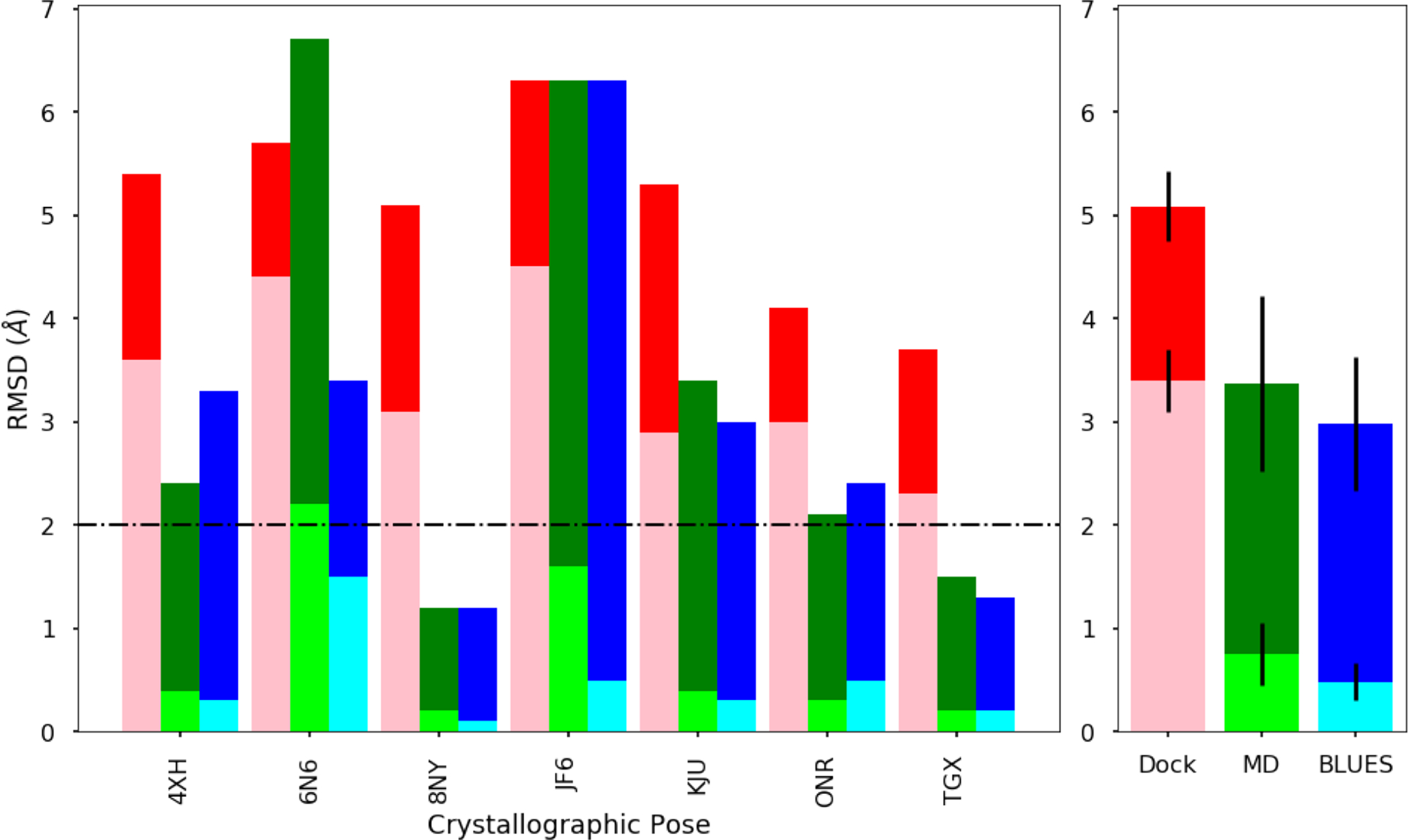
Left: Calculated RMSDs (minimum/average) relative to the crystallographic ligand binding mode and binding modes from docking (pink/red), MD (lime/green), and BLUES (cyan/blue) simulations for ligands with a single binding mode. The lighter shades represent the minimum RMSD and the darker shades represent the average RMSD. Successful prediction in binding mode is judged to be less than or equal to 2Å (black dashed horizontal line). Right: Averaged RMSD for each method: docking, MD, and BLUES for ligands with a single binding mode. Considering the minimum RMSD averaged across ligands with a single binding mode, MD and BLUES can both make predictions with 2Å to the true binding mode.

Table 1:

Calculated RMSD (Å) to the crystal structures for docking, MD, and BLUES. The ‘Side’ column denotes the sub-cavity that the crystallographic binding mode was located in. The ‘Rank’ column denotes the population (% simulation time) rank order of the binding mode for MD and BLUES simulations. The ‘Rank’ column is colored green if the cluster corresponds to the first or second (or third, if there are 3 or more binding modes, per sub-cavity) most populated binding mode and has a minimum RMSD within 2Å; it is colored yellow if it is within 4Å. The ‘Min’ and ‘Avg’ columns denotes the minimum and average RMSDs from the docked poses or cluster of simulation frames. The ‘Err’ column denotes the corresponding error with a 95% confidence interval for the reported average RMSD. The ‘Min’ and ‘Avg’ RMSD columns are colored green to indicate success in sampling the crystallographic binding mode within 2Å and is colored yellow to indicate sampling within 4Å. The population ranking corresponding to the binding modes on this table are also reported in Table 2). Docking generated poses within 2Å of the crystallographic structure in 2/29 (7%) cases. MD recovered the crystallographic binding mode in 14/29 (48%) while BLUES succeeded in 25/29 (86%) cases.

		Dock			MD				BLUES
Ligand	Side	Min	Avg	Err	Rank	Min	Avg	Err	Rank	Min	Avg	Err
4XH	R	3.6	5.4	0	6	0.4	2.4	0.0	2	0.3	3.3	0.0
6N6	L	4.4	5.7	0	4	2.2	6.7	0.1	1	1.5	3.4	0.0
8NY	R	3.1	5.1	0	1	0.2	1.2	0.0	1	0.1	1.2	0.0
JF6	L	4.5	6.3	0	4	1.6	6.3	0.0	2	0.5	6.3	0.1
KJU	R	2.9	5.3	0	3	0.4	3.4	0.0	1	0.3	3.0	0.0
ONR	R	3.0	4.1	0	1	0.3	2.1	0.0	2	0.5	2.4	0.0
TGX	R	2.3	3.7	0	1	0.2	1.5	0.0	1	0.2	1.3	0.0
6TZ1–0	L	4.0	9.1	0.1	1	2.5	8.5	0.1	1	1.7	8.4	0.1
6TZ1–1	R	4.7	7.9	0.1	3	1.5	5.7	0.0	1	1.5	5.6	0.0
6TZ1–2	L	5.1	6.4	0	1	2.6	6.7	0.1	1	1.8	5.3	0.0
6TZ2–0	L	3.9	7.0	0	1	3.6	10.1	0.0	2	1.6	7.4	0.1
6TZ2–1	R	6.2	6.2	0	2	2.3	8.9	0.0	1	1.8	5.5	0.0
6TZ2–2	L	4.3	5.5	0	1	2.3	7.0	0.0	1	0.8	5.6	0.0
GVG1–0	R	3.7	5.5	0	1	0.8	5.0	0.1	2	0.8	3.7	0.0
GVG1–1	R	4.3	5.9	0	1	0.7	5.2	0.1	1	1.6	5.1	0.0
GVG1–2	L	4.3	6.2	0	3	0.6	2.7	0.0	6	0.7	4.1	0.1
GVG1–3	L	1.8	6.3	0.1	1	0.5	2.9	0.1	1	0.5	2.9	0.1
GVG1–4	L	4.9	6.6	0	4	2.4	7.9	0.0	4	1.9	6.0	0.0
GVG2–0	R	4.4	6.1	0	2	0.3	1.4	0.0	1	1.0	2.9	0.0
GVG2–1	R	1.8	4.8	0.1	4	1.5	4.0	0.0	1	1.4	3.9	0.0
GVG2–2	L	4.4	6.5	0	1	2.7	9.1	0.1	2	0.4	6.6	0.1
GVG2–3	L	2.2	6.9	0.1	4	1.3	7.0	0.1	1	0.8	6.5	0.1
GVG2–4	L	4.8	6.7	0	1	1.8	7.7	0.1	1	1.3	6.0	0.0
KUF-0	R	4.9	6.1	0	3	1.4	4.0	0.0	1	1.9	5.8	5.8
KUF-1	R	3.8	4.3	0	2	1.3	5.7	0.0	6	0.9	3.1	0.0
KUF-2	R	2.1	3.6	0	1	0.9	3.5	0.0	1	0.7	3.4	0.0
KUF-3	L	4.0	5.1	0	2	0.9	2.7	0.0	1	0.6	3.1	0.0
KUF-4	L	4.5	6.0	0	1	1.9	8.1	0.0	4	1.3	5.3	0.0
KUF-5	L	6.1	6.6	0	5	1.4	5.5	0.0	3	1.1	4.0	0.0

We also report the minimum RMSD as this represents the best case or ‘ideal’ scenario where we could identify which of our structures (generated from docking or sampled from our simulations) would be closest to the crystallographic binding mode. However, we are not aware of any method which could identify such poses so we view minimum RMSD to be useless as an overall performance metric. Here, we include it simply to provide a way to assess whether any poses sampled were close to the crystallographic binding mode.

To compare the sampling performance between MD and BLUES, we report the rank order (based on population) of the binding mode which is closest to the crystallographic structure. Ideally, with adequate sampling and an accurate force field, the the crystallographic binding mode should be represented by the most populated binding mode sampled during our simulations. In other words, if the binding mode closest to the crystal structure is not the most populated binding modes, this would be indicative of poor sampling performance for that particular method, or of force field errors.

We remind the reader that our analysis treats each sub-cavity separately (Fig. 3). There were a total of 29 crystallographic binding modes identified for the 12 ligands we simulated, because some ligands had multiple binding modes. Molecules fell into 2 groups: those with a single binding mode and those with multiple binding modes (2+). For ligands with a single binding mode, we report the average and minimum RMSDs (described previously) of the ligand atoms in the crystallographic structure against those in the representative frames from the binding mode with the highest occupancy (i.e simulation time). When ligands have multiple crystallographic binding modes, we report the lowest RMSD from the binding modes found from simulations, relative to each crystallographic binding mode.

Here, we define successful predictions as being within 2Å (RMSD) of the crystallographic binding mode and close predictions as those within 4Å of the crystallographic binding mode.

Results

Here, we analyze the success of docking, standard MD and BLUES at recovering crystallographic binding modes for a series of 12 ligands which have a total of 29 binding modes between them. In our analysis, we consider data only from docked poses or binding modes sampled during our simulations which are in the correct sub-cavity. That is, if the crystallographic structure was found in the right sub-cavity, we computed the RMSD using docked poses or simulation frames that were only in the right sub-cavity (and vice versa). In this study, we consider predictions successful when they are within 2Å of the crystallographic binding mode and we label predictions “close” when they are within 4Å.

We remind the reader that we report an ‘average’ RMSD from each method (See Methods: Crystallographic Binding Mode Predictions). Since we cannot determine which docked pose or single simulation frame would result in minimizing the RMSD to the crystallographic binding mode without knowing the crystallographic binding mode, an average RMSD represents the typical accuracy expected from randomly picking from a pool of docked poses or a single simulation frame representative of a metastable binding mode. We also report the minimum RMSD to show the best case or ‘ideal’ scenario for each method. The minimum RMSD reflects the accuracy which would be expected if one could determine somehow, without knowing the crystal structure, which docked pose or simulation frame would be closest to the true binding mode.

The minimum and average RMSDs for each method are reported in Table 1.

As a performance metric, in comparing how well BLUES and MD do at sapling binding modes, we turn to comparing the ranked population of the binding mode closest to the crystal structure, which is reported in Table 2. That is, given sufficient sampling and an appropriate force field, the most populated binding mode should represent the crystallographic binding mode. Here, we also examine a “recovery success rate” which we define as finding the crystallographic binding mode in one of the top two most populated binding modes, as long as the minimum RMSD for this cluster falls below the 2Å cutoff. If there are three or more crystallographic binding modes to identify, we declare success if the crystallographic binding mode is in the top three most populated binding modes.

Table 2:

Rank order based on population (% simulation time) from MD or BLUES simulations of the binding mode closest to the crystallographic structure. The ‘Side’ column denotes the sub-cavity that the crystallographic binding mode was located in. The ‘Start’ column denotes the number of docked poses used for starting the simulations. The ‘BM’ column specifies the total number of binding modes sampled during the MD or BLUES simulations. The ‘CL’ column denotes the index (0-based) of the cluster closest to the crystallographic binding mode and the ‘Color’ column specifies the color. The ‘Rank’ column is colored green if the cluster corresponds to the first or second (or third, if there are 3 or more binding modes, per sub-cavity) most populated binding mode and that the binding mode has a minimum RMSD equal to or less than 2Å; it is colored yellow if the minimum RMSD is between 2 to 4Å. The minimum and average RMSD of each cluster is reported in Table 1. When considering the minimum RMSDs and population rankings, MD was able to recover the crystallographic binding mode in 14/29 (48%) cases but was close in 6/29 (21%) cases; while BLUES was successful finding the crystallographic binding modes in 25/29 (86%) cases.

			MD				BLUES
Ligand	Side	Start	BM	CL	Color	Rank	BM	CL	Color	Rank
4XH	R	2	9	0	red	6	9	7	blue	2
6N6	L	4	6	3	spring green	4	6	5	purple	1
8NY	R	2	7	6	purple	1	3	2	blue	1
JF6	L	4	5	0	red	4	6	4	blue	2
KJU	R	3	8	4	spring green	3	7	4	cyan	1
ONR	R	2	5	4	blue	1	4	3	blue	2
TGX	R	2	4	2	spring green	1	3	2	blue	1
6TZ1–0	L	3	5	1	yellow	1	6	4	blue	1
6TZ1–1	R	2	4	1	yellow	3	6	5	purple	1
6TZ1–2	L	3	5	1	yellow	1	6	4	blue	1
6TZ2–0	L	3	3	1	green	1	5	2	green	2
6TZ2–1	R	2	7	4	cyan	2	6	5	purple	1
6TZ2–2	L	3	3	1	green	1	5	3	cyan	1
GVG1–0	R	3	5	3	cyan	1	6	4	blue	2
GVG1–1	R	3	5	3	cyan	1	6	0	green	1
GVG1–2	L	3	5	3	cyan	3	8	3	green	6
GVG1–3	L	3	5	4	blue	1	8	7	purple	1
GVG1–4	L	3	5	2	green	4	8	0	red	4
GVG2–0	R	2	4	2	spring green	2	3	1	green	1
GVG2–1	R	2	4	0	red	4	3	1	green	1
GVG2–2	L	4	6	3	spring green	1	6	5	purple	2
GVG2–3	L	4	6	4	blue	4	6	4	blue	1
GVG2–4	L	4	6	3	spring green	1	6	4	blue	1
KUF-0	R	2	7	4	cyan	3	8	1	purple	1
KUF-1	R	2	7	3	green	2	8	6	red	6
KUF-2	R	2	7	6	purple	1	8	1	purple	1
KUF-3	L	4	6	5	purple	2	9	8	purple	1
KUF-4	L	4	6	4	blue	1	9	5	cyan	4
KUF-5	L	4	6	2	green	5	9	6	sky blue	3

Analysis of Molecules with a Single Binding Mode

Molecules with a single crystallographic binding mode were 4XH, 6N6, 8NY, JF6, KJU, ONR, and TGX. Calculated RMSDs are measured in units of Å and are shown in Figure 10 and reported in Table 1. The rankings of the binding modes closest to the crystallographic structure are reported in Table 2.

When considering the minimum RMSDs from docking, we see that docking can generate poses which are only close (within 4Å) to the crystallographic structure for molecules 4XH, 8NY, KJU, ONR, and TGX (Table 1). None of the poses generated from docking were within our success cutoff of 2Å to the crystal structure. This suggests that docking may be good for generating simulation starting configurations as the simulations would start off fairly close to the crystallographic structure.

From Table 2, we show the rankings (based on % simulation time) of the MD/BLUES binding modes which are closest to the crystallographic binding mode. For this subset of single binding mode molecules, the most populated binding modes from MD corresponded with the crystal structure in 3/7 cases which are from molecules 8NY, ONR, TGX. For MD simulations of 8NY and TGX, both the minimum and average RMSD are within the 2Å cutoff for the most populated binding mode. This indicates that the most populated binding modes were well defined and are in good agreement with the crystallographic binding mode (Fig. 10, Table 1). For MD simulations of ONR, the minimum RMSD was calculated to be 0.3Å, which suggests that we were able to sample the crystallographic binding mode. But, the average RMSD for this binding mode was 2.1Å which suggests that the binding mode may not be as well defined or that the forcefield used prefers a binding mode which is close (within 4Å) to the crystal structure (Fig. 10, Table 1).

From our BLUES simulations, the most populated binding mode corresponded with the crystal structure in 4/7 cases but in the remaining 3/7 cases, the second most populated binding mode represented the crystallographic binding mode. In all 7/7 single binding mode cases, the minimum RMSD from BLUES simulations were all below the 2Å cutoff, indicating that BLUES can indeed sample the crystallographic binding mode and does so more successfully than standard MD. But, only molecules 8NY and TGX appeared to be well defined and in close agreement with the crystal structure as the average RMSD for these molecules fell below 2Å. For molecules 4XH, 6N6, KJU, and ONR, the binding modes were less well defined or had slight disagreement with the crystal structure with average RMSDs that were below our 4Å cutoff. Lastly, JF6 had a very high average RMSD of 6.3Å indicating that the binding mode was poorly defined or that the forcefield disagreed with the crystallographic binding mode.

Across this subset of molecules with a single binding mode, the minimum RMSDs for docking (pink), MD (lime), and BLUES (cyan), were 3.4 ± 0.3Å, 0.8 ± 0.3Å, and 0.5 ± 0.2Å respectively; average RMSDs for docking (red), MD (green), and BLUES (blue) were 5.1±0.3Å, 3.4 ± 0.9Å, and 3.0 ± 0.6Å respectively (Fig. 10, right). Thus, based on considering the overall minimum RMSD, docking will often generate poses which are close (within 4Å) to the crystallographic binding mode. Using these docked poses as starting points, further exploration via either MD or BLUES simulations here easily generates samples which are representative of the crystal structure (Fig. 10, Table 1). But, here, only BLUES simulations generate trajectories which spend most of the simulation time in the binding modes which represents the crystallographic binding mode (Table 2), due to slower transitions between binding modes in the MD simulations. With longer MD simulations, we expect results could become comparable, with significant additional sampling expense.

When we consider the overall average RMSD from each method, we can see that docked poses will be quite far from the crystal structure on average. On the other hand–given that we can at least sample the crystallographic binding mode using MD or BLUES–when a modeller tries to select a specific sample or simulation frame (from the most populated cluster) to compare against the crystal structure, they will on average select a sample which is at least within 4Å to the crystallographic binding mode.

Analysis of Molecules with Multiple Binding Modes

Molecules with multiple binding modes were 6TZ(1/2), GVG(1/2), and KUF which had 3, 5, and 6 crystallographic binding modes, respectively. Some molecules had uncertain tautomers, which we reflect in our notation. Specifically, 6TZ(1/2) denote two possible tautomers of 6TZ, and similarly for or GVG(1/2). We consider these separately as we were uncertain which tautomers would actually be dominant in binding to this target, and thus which we should simulate both.

We compare binding modes sampled in simulations of 6TZ(1/2) and GVG(1/2) to the same crystallographic structure regardless of which tautomer we were simulating, since protons are not resolved in the crystal structures. The RMSD for each molecule to each crystallographic structure is denoted as XXXX-#; for example, 6TZ1-(0,1,2) is the comparison from the simulations of 6TZ1 against each of the 3 crystallographic binding modes.

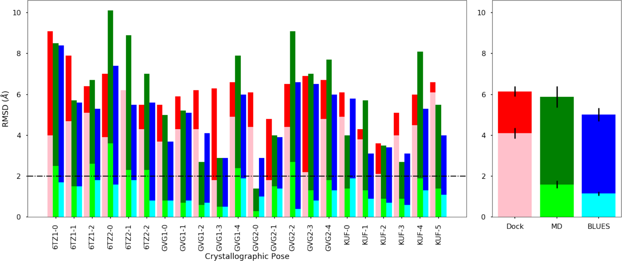
For this subset of ligands with multiple binding modes, the collective minimum RMSD was 4.1 ± 0.3, 1.6 ± 0.2, and 1.2 ± 0.1 from docking, MD, and BLUES, respectively. The collective average RMSD was 6.1±0.2, 5.9±0.5, and 5.0±0.3 from docking, MD and BLUES, respectively. When considering the minimum RMSD, docking can generate poses which are close (within 4Å) to the crystallographic structures, even if there are multiple binding modes. With MD and BLUES, we found that we were able to generate samples which are within 2Å of the crystallographic binding modes.

Analysis of Simulations of 6TZ(1/2)

For 6TZ(1/2), there were two crystallographic binding modes in the left sub-cavity (6TZ-0/2) and one in the right sub-cavity (6TZ-1). From Table 1 and Figure 11, the minimum RMSDs of 6TZ1 to the crystallographic structures were 4.0, 4.7, and 5.1 from docking; 2.5, 1.5, and 2.6 from MD; and 1.7, 1.5, and 1.8 from BLUES. The average RMSDs were reported to be 9.1, 7.9, and 6.4 from docking; 8.5, 5.7, and 6.7 from MD; and 8.4, 5.6, and 5.3 from BLUES. In the case of 6TZ1, docking had generated one pose which was close to one crystal structure (6TZ-0) and was far away from the other crystal structures.

Figure 11:

Left: Calculated RMSDs (minimum/average) relative to the crystallographic ligand binding mode and binding modes from docking (pink/red), MD (lime/green), and BLUES (cyan/blue) simulations for ligands with a single binding mode. The lighter shades represent the minimum RMSD and the darker shades represent the average RMSD. Successful prediction in binding mode is judged to be less than or equal to 2Å (black dashed horizontal line). Right: Averaged RMSDs for each method: docking, MD, and BLUES for ligands with a single binding mode. Considering the minimum RMSD averaged across ligands with a single binding mode, BLUES can make predictions with 2Å to the true binding mode.

From Table 2, we see that the single most populated binding mode from MD and BLUES corresponds to the two crystal structures 6TZ-0 and 6TZ-2, which were located in the left sub-cavity. This suggests that our clustering approach was unable to distinguish two separate binding modes in the left sub-cavity and instead defined a single binding mode which resembled something in between both of them. From MD (Table 1), the minimum RMSDs relative to 6TZ-(0/2) from the most populated MD binding mode (yellow, Fig. S32) was only close to the crystallographic binding mode (2.5Å and 2.6Å). Thus, we do not count this as successfully sampling the crystallographic structure but claim MD had sampled fairly close to it.

From BLUES (Table 1), the minimum RMSD for the most populated binding mode in the left sub-cavity (blue, Fig. S34) and right sub-cavity (purple, Fig. S38) were below our 2Å cutoff. This indicates that with BLUES simulations of 6TZ1, we were successfully able to generate samples which were representative of all 3 crystallographic binding modes. Despite the low minimum RMSDs, the average RMSDs were quite high (above 4Å), suggesting that the BLUES binding modes for 6TZ1 were poorly defined or the simulations simply disagree with the crystallographic results. Such a high average RMSD would indicate that it would be challenging for a modeller to pick the specific sample (i.e. simulation frame) which would be closest to the crystal structure.

In the case of 6TZ2, the minimum RMSDs were 3.9, 6.2, and 4.3 from docking; 3.6, 2.3 and 2.3 from MD; and 1.6, 1.8, and 0.8 from BLUES. The average RMSDs were reported to be 7.0, 6.2, and 5.5 from docking; 10.1, 8.9, and 7.0 from MD; and 7.4, 5.5, and 5.6 from BLUES (Table 1 and Fig. 11). Here, docking generated one pose which was 3.9Å away from crystal structure 6TZ-0 and was far away for the rest.

For MD simulations of 6TZ2 in the left sub-cavity, the most populated binding mode (green, Fig. S40) was only close (within 4Å) to the crystal structures 6TZ-(0/2). Like in the case of 6TZ1, our clustering approach was unable to define two separate binding modes for each crystal structure and instead defined a binding mode which was close to both 6TZ-(0/2) (Table 2, 1). For MD simulations of 6TZ2 in the right sub-cavity, the binding mode closest to the crystal structure 6TZ-1 corresponded to the 2nd most populated binding mode (cyan, Fig. S44) and was only close to the crystallographic binding mode (2.3Å). Here, MD simulations of 6TZ2 failed to recover the crystallographic binding mode and were only able to sample close to it.

In BLUES simulations of 6TZ2 in left sub-cavity, the most populated binding mode (cyan, Fig. S42) was at minimum 0.8Å away from crystal structure 6TZ-2 and the second most populated binding (green, Fig. S42) was at minimum 1.6Å away from crystal structure 6TZ-0. For the right sub-cavity, the most populated binding mode (purple, Fig.S46) was at minimum 1.8Å away from crystal structure 6TZ-1. These results indicate that BLUES was able to generate samples which were representative of the crystallographic binding modes 6TZ-(0,1,2) for all 3 cases. However, all the average RMSDs for the BLUES binding modes were higher than 4Å which would suggest that these binding modes were poorly defined or that the forcefield disagrees with the crystal structures.

When we consider the minimum RMSDs, we find that the dominant MD binding modes sampled only close to the crystal structure in 2/3 cases for 6TZ1 and in 3/3 cases for 6TZ2. On the other hand, the dominant BLUES binding modes produced samples which were representative (below 2Å) of the crystallographic structure in all cases for both 6TZ1 and 6TZ2. But, the dominant BLUES binding modes had high average RMSDs, which suggests that there is disagreement with the crystal structure or that the clusters were poorly defined. From these results alone, we cannot definitively say which tautomer for 6TZ is likely to dominate in the binding site, as both produced reasonable agreement with the crystal structure. But based on Fig. S41 and S43), we observe more stabilized sampling of (or near) the crystallographic binding mode in simulations of 6TZ2; thus, we believe 6TZ2 may be the dominant tautomer in the binding site.

Analysis of Simulations of GVG(1/2)

For molecule GVG, we simulated two tautomers which are denoted as GVG1 or GVG2. There were a total of 5 crystallographic binding modes where 2 were located in the right sub-cavity, denoted as GVG1-(0,1) or GVG2-(0,1), and 3 located in the left sub-cavity, denoted with GVG1-(2,3,4) or GVG2-(2,3,4). We first present the results for GVG1 and then discuss the results from GVG2.

For the right sub-cavity, we see that docking had generated poses close to GVG1–0 (within 3.7Å) but was 4.3Å away from GVG1–1 (Table. 1). Given that at least one pose was close to the crystal structure GVG1–0, both MD and BLUES were able to recover the binding mode GVG1–0 within the top two most populated binding modes. The most populated MD binding mode (cyan, Fig. S48), had a minimum RMSD of 0.8Å to GVG1–0 and 0.7Å to GVG1–1 (Table 1, Fig. S49), indicating that we have indeed sampled both crystallographic binding modes. In this case, our clustering approach from our MD simulations defined a single binding mode which was close to both crystallographic binding modes, GVG-(0,1). On the other hand, BLUES defined two separate binding modes which corresponded with each crystal structure. The second most populated BLUES binding mode (blue, Fig. S50) was representative of the crystallographic structure GVG-0 with a minimum RMSD of 0.8Å (Table 1, Fig. S51). The most populated binding (green, Fig. S50) mode was able to sample crystal structure GVG-1 with a minimum RMSD of 1.6Å. Thus, for the right sub-cavity, MD was able to recover 2/2 binding modes while BLUES was only able to recover 2/2 binding modes for GVG1.

When we consider the left sub-cavity, there were 3 crystallographic binding modes to identify GVG1-(2,3,4). In this case, we consider the recovery success rate when either the top three most populated binding modes are able to sample close to the crystallographic binding mode. For crystal structures GVG1-(2,4), poses generated from docking were 4.3 and 4.9Å away and the closest docked pose was 1.8Å away from GVG1–3. From MD binding modes, we were able to sample the crystallographic binding modes GVG1–2 and GVG1–3 with the third (cyan) and first (blue) most populated binding modes (Table. 2, Fig. S52). Here, the closest samples generated from MD were 0.6Å away from GVG1–2 and 0.5Å away from GVG1–3 (Fig. S53). In the case of GVG1–4, the fourth most populated MD binding mode (green) had sampled fairly close to the crystal structure at a distance of 2.4Å away. In our BLUES binding modes, we see only success in sampling GVG1–3, where a sample from the most populated binding mode (purple, Fig. S54) was 0.5Å away from the crystal structure (Fig. S55). For GVG1–2 and GVG1–4, BLUES was able to sample 0.7 and 1.9Å away from the crystal structures, respectively. But, these samples came out of the sixth and fourth most populated binding modes. Thus, for the left sub-cavity, MD was able to recover 2/3 binding modes and BLUES was able to recover 1/3 binding modes for GVG1.

When considering the right sub-cavity for GVG2, the closest docked pose was 1.8Å away from GVG2–1 and was 4.4Å away from GVG-0. The second most populated MD binding mode (spring green, Fig. S56) was able to sample the crystallographic binding mode GVG2–0 at 0.3Å away (Fig. S57). Our clustering approach from our BLUES simulations resulted in defining a single dominant binding mode (green, Fig. S58) which was 1.0 and 1.4Å away from crystal structures GVG2–0 and GVG2–1, respectively. Thus, for the right sub-cavity, MD recovered 1/2 cases and BLUES recovered 2/2 cases for GVG2.

For GVG2 binding modes in the left sub-cavity, docking generated poses which were 4.4, 2.2, and 4.8Å away from crystal structures GVG2-(2,3,4), respectively. From our MD simulations, the most populated binding mode (spring green, Fig. S60) came close to GVG2–2 at 2.7Å but was successful in sampling GVG2–4 at 1.8Å away (Table. 1, Fig.S61). Similarly, in our BLUES simulations, the most populated binding mode (blue, Fig.S62) was successful in sampling GVG2–3 and GVG-4 at 0.8 and 1.3Å away from the crystal structure (Fig. S63). The second most populated BLUES binding mode (purple. Fig.S62) was able to sample 0.4Å away from crystal structure GVG2–2. Thus, for the left sub-cavity, MD recovered 2/3 binding modes while BLUES recovered 3/3 binding modes for GVG2. From our results, we believe simulation of GVG2 were the correct tautomeric state as we were able to recover more of the crystallographic binding modes in simulations of GVG2 over GVG1.

Analysis of Simulations of KUF

For molecule KUF, there were a total of 6 crystallographic binding modes to identify where KUF-(0,1,2) refer to the binding modes located in the right sub-cavity and KUF-(3,4,5) refer to the binding modes located in the left sub-cavity. For the right sub-cavity, docking had generated poses which were close to the crystal structures of KUF-1 and KUF-2 at 3.8 and 2.1Å away, respectively; while the closest pose to KUF-0 was 4.9Å away (Table 1). For the left sub-cavity, docking only came close to crystal structure KUF-3 at 4Å away and was much further away for KUF-4 and KUF-5 at 4.5 and 6.1Å away, respectively (Table 1).

In our MD simulations of KUF, we were able to recover the crystallographic binding modes in the right sub-cavity for all 3 cases KUF-(0,1,2) from the top three most populated binding modes (Table. 2). From Fig. S65, we see that the most populated binding mode (purple, Fig. S64) was able to sample the crystallographic binding mode KUF-2 at 0.9Å. The second (green) and third (cyan) most populated binding modes, corresponded with crystal structures KUF-0 and KUF-1, respectively (Fig.S64). The green binding mode was closest to the crystal structure KUF-1 with minimum RMSD of 1.3Å, while the cyan binding mode was closest to crystal structure KUF-2 with a minimum RMSD of 1.4Å (Table. 1, Fig.S65). In the case of BLUES binding modes, a single dominant binding mode (purple, Fig. S66) generated samples which were 1.9Å away from KUF-0 and 0.7Å away from KUF-2. For KUF binding modes in the right sub-cavity, MD successfully able to sample all 3/3 crystallographic structures KUF-(0,1,2) while BLUES was only able to sample 2/3 cases (KUF-0 and KUF-2).

When considering KUF binding modes in the left sub-cavity (KUF-3,4,5), docking had generated a pose which was close to the crystal structure KUF-3 by 4Å but was 4.5 and 6.1Å away from KUF-4 and KUF-5, respectively (Table 1). From our MD binding modes, the top two most populated binding modes (blue and purple, Fig. S68), corresponded with crystal structures KUF-3 and KUF-4 (Table 2). The most populated binding mode (blue) contained a sample which was representative of the crystal structure KUF-4 at a distance of 1.9Å away; while the second most populated (purple) binding mode represented crystal structure KUF-3 at a distance of 0.9Å away (Fig. S69). In the case of KUF-5, MD failed to recover this crystallographic binding mode, where the fifth most populated binding mode corresponded with the crystal structure at a distance of 1.4Å. From our BLUES binding modes, the first and third binding mode (purple and sky blue, Fig. S70) corresponded with the crystal structures KUF-3 and KUF-5, respectively. The purple binding mode from BLUES contained a sample with a minimum RMSD of 0.6Å from KUF-3 and the sky blue binding mode contained a sample which was 1.1Å away from KUF-5 (Fig. S71). For KUF-4, the fourth most populated binding mode from our BLUES simulations contained a sample with a minimum RMSD of 1.3Å away. Thus, for KUF binding modes in the left sub-cavity, both MD and BLUES were able to recover 2/3 cases where MD found KUF-3 and KUF-4 and BLUES found KUF-3 and KUF-5.

Dataset Summary

Here, we find that no method always correctly identifies the crystallographic binding mode (as evidenced by average RMSD) but both MD and BLUES substantially outperform docking at sampling binding modes near the crystallographic one, and of these, BLUES performs better. From Table 1, we see that docking was only able to generate poses which were within 2Å of the crystallographic structure in 2/29 (7%) cases and was close (within 4Å) in 12/29 (41%) cases. To remind the reader, when we evaluate the sampling proficiency for MD and BLUES, we consider the method successful when the top two most populated binding modes (or top three if there are 3 or more crystallographic binding modes) contain a sample which is within 2Å of the crystal structure (Table 2). Across the all the molecules used in this study, MD was able to recover the crystallographic binding mode in 14/29 (48%) cases but was close in 6/29 (21%) cases; while BLUES was successful finding the crystallographic binding modes in 25/29 (86%) cases.

Averaged across all of the ligands in this study, the minimum RMSDs for docking (pink), MD (lime), and BLUES (cyan) were 3.9 ± 0.2Å, 1.4 ± 0.2Å, and 1.0 ± 0.1Å respectively; the average RMSD for docking (red), MD (green), and BLUES were 5.9 ± 0.2Å, 5.3 ± 0.5Å, and 4.5 ± 0.3Å respectively ((Fig. 12). On average, when considering both cases of single and multiple crystallographic binding modes to identify, none of the 3 methods considered here appear to make predictions which are close (within 4Å) to the crystallographic binding mode. At best (considering the minimum RMSD), both MD and BLUES simulations may be able to generate samples which are at least within 2Å to the crystallographic binding mode. But, when we factor in the binding mode populations, we can clearly see that BLUES out performs standard MD simulations at recovering the crystallographic binding mode. We note that the average RMSD is a poor metric as there is no physical reason why the average RMSD of a ‘perfect’ method ought to be low. The most meaningful metric here is that the most populated binding modes from either simulation method corresponds well with the crystal structure.

Figure 12:

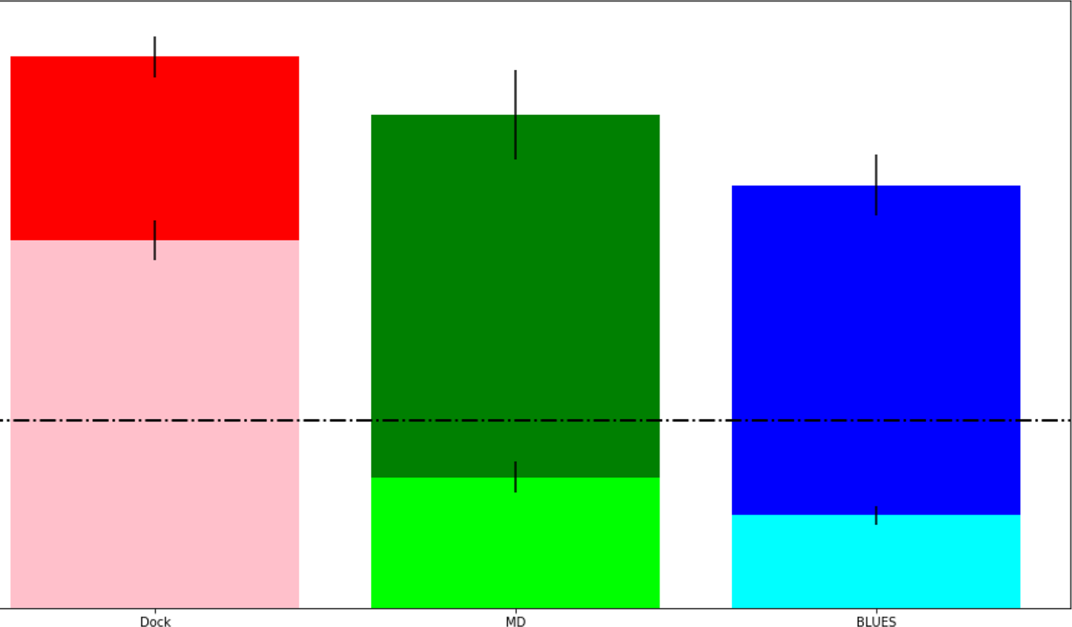
Minimum/Average RMSD for each method: docking (pink/red), MD (lime/green), and BLUES (cyan/blue) for all ligands in this study. Dashed line at 2Å represents successful predictions and dotted line at 4Å represents close predictions. This reports the averaged RMSD from all 12 ligands used in this study.

Discussion

Single Binding Mode: BLUES recovers the crystallographic binding mode faster and better than MD

For molecules which exhibit only a single binding mode (molecules: 4XH, 6N6, 8NY, JF6, KJU, ONR, and TGX), we see from Table 1 and Table 2, that MD is only able to recover 3/7 binding modes while BLUES is able to recover all 7/7 binding modes. In general, we find that through using BLUES simulations, we are able to recover the crystallographic binding mode much faster than standard MD. In some cases (e.g. 8NY, ONR, TGX) MD was able to quickly recover the crystallographic binding mode as docking had generated nearby starting poses (within 4Å).

If we were to only consider the minimum RMSDs, we find that MD is at least able to sample the crystallographic binding mode (within 2Å) in all cases but 6N6. Where MD falls short is in populating the binding mode which is representative of the crystallographic binding mode. Given sufficient sampling time and accurate forcefields, the most populated binding modes should correspond to the crystal structure which we find to be the case when using BLUES rather than standard MD due to the enhanced sampling we get using the BLUES approach.

From BLUES, the first or second most populated binding mode corresponded with the crystal structure in all single binding mode cases, which was not the case when using MD. We find that in cases where both methods are able to find the crystallographic binding mode quickly, MD has a tendency to not produce the expected populations. This is because when MD samples the crystallographic binding mode and then leaves, it has a tendency to not rediscover it (e.g 4XH, JF6, KJU). Ideally, if the crystallographic structure represents the most stable binding mode, both MD and BLUES should populate that binding mode the most. However, if timescales for transition between binding modes are very slow (as is especially the case with MD) this may not be the case on the timescale of any reasonable simulation – as we find here. Given that our BLUES approach proposes random rotational moves on the ligand every 200ps, we did not expect the ligand to remain trapped in the crystallographic binding mode like we did with MD. Thus, this highlights that with BLUES, not only are we able to sample the crystal structure but we are able to recover the correct populations–unlike with MD.

Multiple Binding Mode: BLUES transiently samples the crystallographic binding mode

Here, we separately analyze compounds which exhibit multiple crystallographic binding modes simply because such cases require different analysis approaches. However, we note that it is impossible to know–a priori–if molecules would bind in a single binding mode versus multiple binding modes, as determined by crystallography.

In general, analysis of X-ray crystallography will tend to capture only the dominant binding mode(s) – though our re-refinement here avoids some of these typical limitations. Specifically, we deliberately re-refined the structures in this study in an attempt to specifically detect lower occupancy binding modes.

Here we deliberately avoid discussing potentially confounding factors that might impact agreement between binding modes observed from simulation, and those observed from crystallography, because such differences are not within the scope of our study. These include differences due to cryogenic temperatures for crystals, effects from crystal packing, co-solvent effects in crystals, and protein force field limitations,⁶⁰ which could further impact binding modes.

For these molecules which exhibit multiple crystallographic binding modes, MD was able to recover 11/22 (50%) of the crystallographic binding modes while BLUES was able to resolve 17/22 (77%). This doesn’t suggest that BLUES is more successful in recovering crystallographic binding modes if there are multiple ones to identify. We generally observed that both MD and BLUES were able to stably sample at least 1 of the crystallographic binding modes, while only briefly sampling (or sampling close to) the second or third binding mode. Here, BLUES and MD result in equivalent performance as measured by how often the crystallographic binding mode matches the most populated binding mode. However, BLUES does do a better job transiently sampling the crystallographic binding mode even in those cases where MD does not discover it. Thus, BLUES is more successful at discovering crystallographic binding modes in general, which is not surprising given that it employs rotational moves to better explore possible binding modes. It is interesting that in some of these cases, BLUES discovers the crystallographic binding mode but stabilizes into an alternate nearby mode, potentially due to force field errors.

In the case of MD, the simulations have a tendency to stabilize into a binding mode which is close to the crystal structure, rather than sampling close to the crystallographic structure. In general, we believe this may be due to the forcefield disagreeing with some of the crystal structure–particularly in the case of 6TZ. This discrepancy could also be because of differences in conditions (crystallographic structures being collected at cryogenic temperatures, for example, and in the environment of a crystal). Clusters for molecules which have a single binding mode have an overall average RMSD of 3.4 ± 0.9Å from MD and 3.0 ± 0.6Å from BLUES, while clusters for molecules with multiple binding modes have an overall average RMSD of 5.9 ± 0.5Å from MD and 5.0 ± 0.3Å. We believe that the higher average RMSD for multiple binding mode molecules (6TZ, GVG, KUF) may suggest that converged forcefield results disagree with the crystallographic binding modes. This may indicate deficiencies in the forcefield or differences in simulation conditions relative to crystallographic conditions, as discussed above.

Conclusions

In this study, we evaluated several potential techniques for predicting fragment binding modes, as judged by comparison to crystallographic bound structures. Specifically, we compared the performance of docking, MD, and (NCMC+MD) BLUES at recovering crystallographic binding modes for a set of fragment-like molecules bound to soluble-epoxide hydrolase (SEH). We assessed how well these approaches do at sampling the crystallographic structure, but also how well they do (in the case of BLUES and MD) at recognizing the crystallographic binding mode as the most populated binding mode out of several possibilities.

Here, our reported minimum RMSDs illustrate the ability to sample the crystallographic structure and our reported average RMSDs serve as a representation of how well our clustering algorithm defines a particular binding mode and if our approach in general agrees with the crystallographic binding modes. For docking, the poses chosen by our MDS-RMSD filtering approach were often within 4Å of the crystallographic structure and in rare cases were within 2Å.

When comparing MD and BLUES, we found that both approaches perform roughly equivalently in being able to sample the crystallographic binding mode within 2Å RMSD. BLUES, however, performs much better than standard MD in recovery success rate – that is, finding the crystallographic binding mode in the top two most populated binding modes. This demonstrates that we are indeed able to enhance ligand binding mode sampling using our BLUES approach while also obtaining closer to correct populations.

Overall, we showed that microsecond MD simulations of small fragment-like molecules in the large SEH binding site were unable to adequately sample ligand binding mode transitions, even within a given sub-cavity, which resulted in MD failing to produce correct populations. Only by accelerating the sampling using random ligand rotations via our BLUES approach were we able to recover binding mode populations which correctly identified crystallographic binding modes in most cases. While MD did do better than docking at discovering crystallographic binding modes, even with the relatively long MD simulation time, we found most MD simulations remained trapped in or near a binding mode other than the crystallographic binding mode and, often, relatively near the starting dock pose. Since these simulations often remained trapped, our conclusion is that the best general approach is to use a variety of starting poses from docking to get good coverage of the binding site and run simulations to refine the pose such that it can recover likely potential binding modes, including potentially the crystallographic binding mode.

Using BLUES, we were able to enhance the sampling of ligand binding modes over traditional MD and found that BLUES often discovers the crystallographic binding mode with shorter simulation times and does a better job ensuring the dominant binding mode is well populated in simulations. Ultimately, enhanced sampling via BLUES lead to an improvement in finding the crystallographic binding modes over traditional MD simulations.

Figure 2:

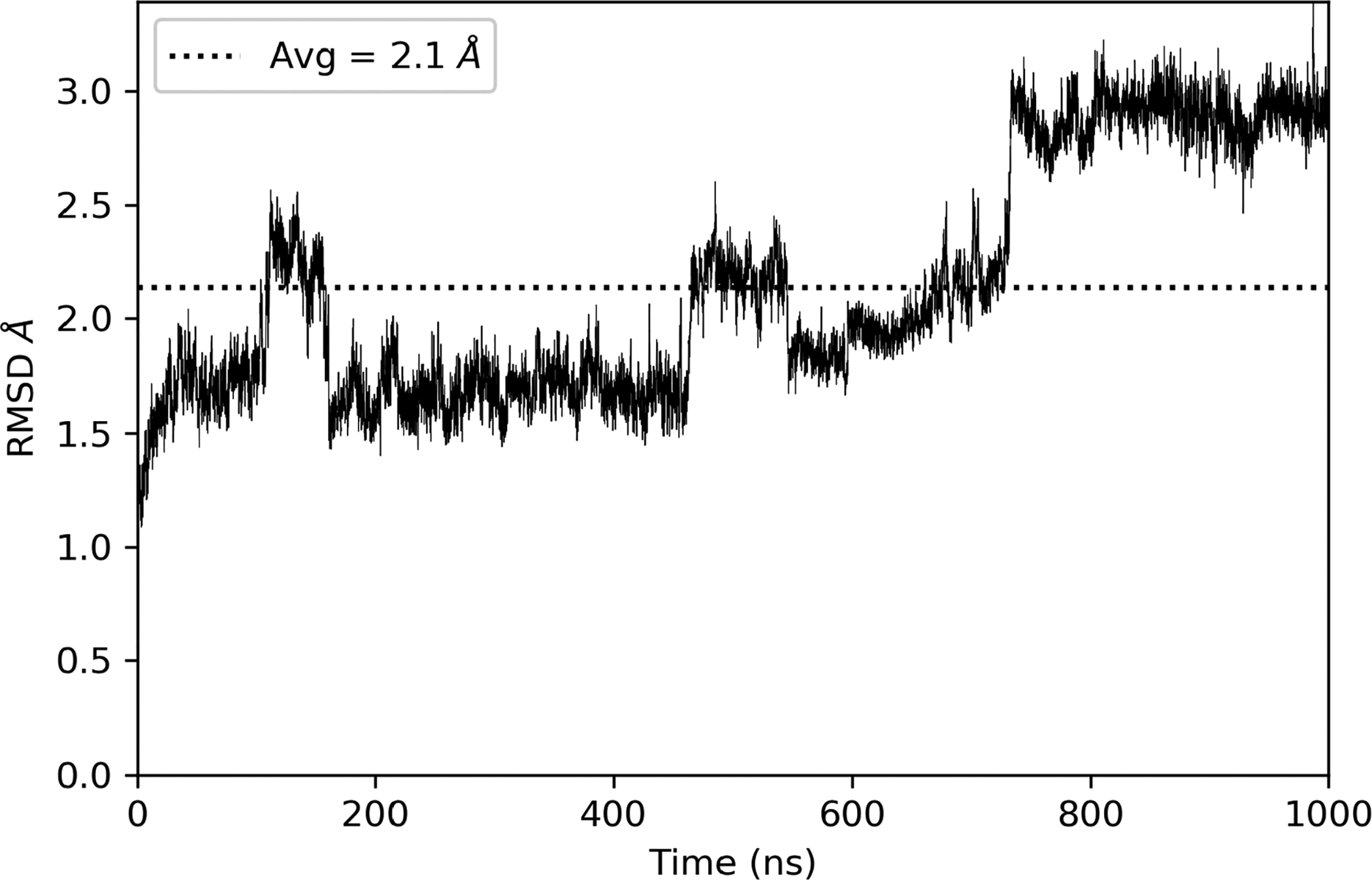
Calculated RMSD (Å) of the protein backbone relative to the starting position for 1 microsecond of MD with an average RMSD of 2.1Å after removal of the N-terminal domain. The protein backbone eventually stabilizes at 3Å from the starting position. This indicates that removal of the N-terminal domain did not largely affect the protein structure.

References

- 1.Erlanson DA In Fragment-Based Drug Discovery and X-Ray Crystallography; Davies TG, Hyvönen M, Eds.; Topics in Current Chemistry; Springer Berlin Heidelberg: Berlin, Heidelberg, 2012; pp 1–32. [DOI] [PubMed] [Google Scholar]
- 2.Erlanson DA; Wells JA; Braisted AC Tethering: Fragment-Based Drug Discovery. Annual Review of Biophysics and Biomolecular Structure 2004, 33, 199–223. [DOI] [PubMed] [Google Scholar]
- 3.Jhoti H; Cleasby A; Verdonk M; Williams G Fragment-based screening using X-ray crystallography and NMR spectroscopy. Current Opinion in Chemical Biology 2007, 11, 485–493. [DOI] [PubMed] [Google Scholar]
- 4.Gozalbes R; Carbajo, R. J; Pineda-Lucena A Contributions of Computational Chemistry and Biophysical Techniques to Fragment-Based Drug Discovery. 2010; https://www.ingentaconnect.com/content/ben/cmc/2010/00000017/00000017/art00003. [DOI] [PubMed] [Google Scholar]
- 5.Domagalski MJ; Zheng H; Zimmerman MD; Dauter Z; Wlodawer A; Minor W The Quality and Validation of Structures from Structural Genomics. Methods in molecular biology (Clifton, N.J.) 2014, 1091, 297–314. [DOI] [PMC free article] [PubMed] [Google Scholar]
- 6.Rocklin GJ; Boyce SE; Fischer M; Fish I; Mobley DL; Shoichet BK; Dill KA Blind prediction of charged ligand binding affinities in a model binding site. Journal of molecular biology 2013, 425, 4569–4583. [DOI] [PMC free article] [PubMed] [Google Scholar]
- 7.Durrant JD; McCammon JA Computer-aided drug-discovery techniques that account for receptor flexibility. Current Opinion in Pharmacology 2010, 10, 770–774. [DOI] [PMC free article] [PubMed] [Google Scholar]
- 8.Sliwoski G; Kothiwale S; Meiler J; Lowe EW Computational Methods in Drug Discovery. Pharmacological Reviews 2014, 66, 334–395. [DOI] [PMC free article] [PubMed] [Google Scholar]
- 9.Lape M; Elam C; Paula S Comparison of current docking tools for the simulation of inhibitor binding by the transmembrane domain of the sarco/endoplasmic reticulum calcium ATPase. Biophysical chemistry 2010, 150, 88–97. [DOI] [PMC free article] [PubMed] [Google Scholar]
- 10.Plewczynski D; Ła¹niewski M; Augustyniak R; Ginalski K Can we trust docking results? Evaluation of seven commonly used programs on PDBbind database. Journal of Computational Chemistry 2011, 32, 742–755. [DOI] [PubMed] [Google Scholar]
- 11.Ramírez D; Caballero J Is It Reliable to Take the Molecular Docking Top Scoring Position as the Best Solution without Considering Available Structural Data? Molecules : A Journal of Synthetic Chemistry and Natural Product Chemistry 2018, 23. [DOI] [PMC free article] [PubMed] [Google Scholar]
- 12.Gohlke H; Hendlich M; Klebe G Knowledge-based scoring function to predict protein-ligand interactions11Edited by R. Huber. Journal of Molecular Biology 2000, 295, 337–356. [DOI] [PubMed] [Google Scholar]
- 13.Warren GL; Andrews CW; Capelli A-M; Clarke B; LaLonde J; Lambert MH; Lindvall M; Nevins N; Semus SF; Senger S; Tedesco G; Wall ID; Woolven JM; Peishoff CE; Head MS A Critical Assessment of Docking Programs and Scoring Functions. Journal of Medicinal Chemistry 2006, 49, 5912–5931.17004707 [Google Scholar]
- 14.Pagadala NS; Syed K; Tuszynski J Software for molecular docking: a review. Biophysical reviews 2017, 9, 91–102. [DOI] [PMC free article] [PubMed] [Google Scholar]
- 15.Guedes IA; de Magalhães CS; Dardenne LE Receptor–ligand molecular docking. Biophysical Reviews 2013, 6, 75–87. [DOI] [PMC free article] [PubMed] [Google Scholar]
- 16.Hospital A; Goñi JR; Orozco M; Gelpí JL Molecular dynamics simulations: advances and applications. Advances and Applications in Bioinformatics and Chemistry : AABC 2015, 8, 37–47. [DOI] [PMC free article] [PubMed] [Google Scholar]
- 17.Hollingsworth SA; Dror RO Molecular Dynamics Simulation for All. Neuron 2018, 99, 1129–1143. [DOI] [PMC free article] [PubMed] [Google Scholar]
- 18.Hopkins CW; Le Grand S; Walker RC; Roitberg AE Long-Time-Step Molecular Dynamics through Hydrogen Mass Repartitioning. Journal of Chemical Theory and Computation 2015, 11, 1864–1874. [DOI] [PubMed] [Google Scholar]
- 19.Han K.-l., Zhang X, Yang M.-j., Eds. Protein Conformational Dynamics; Advances in Experimental Medicine and Biology; Springer International Publishing, 2014. [Google Scholar]
- 20.Schlick T; Barth E; Mandziuk M BIOMOLECULAR DYNAMICS AT LONG TIMESTEPS:Bridging the Timescale Gap Between Simulation and Experimentation. Annual Review of Biophysics and Biomolecular Structure 1997, 26, 181–222. [DOI] [PubMed] [Google Scholar]
- 21.Macek P; Novák P; Žídek L; Sklenář V Backbone Motions of Free and Pheromone-Bound Major Urinary Protein I Studied by Molecular Dynamics Simulation. The Journal of Physical Chemistry B 2007, 111, 5731–5739. [DOI] [PubMed] [Google Scholar]
- 22.Giovannelli E; Gellini C; Pietraperzia G; Cardini G; Chelli R Nonequilibrium Candidate Monte Carlo Simulations with Configurational Freezing Schemes. Journal of Chemical Theory and Computation 2014, 10, 4273–4283. [DOI] [PubMed] [Google Scholar]
- 23.Gill SC; Lim NM; Grinaway PB; Rustenburg AS; Fass J; Ross GA; Chodera JD; Mobley DL Binding Modes of Ligands Using Enhanced Sampling (BLUES): Rapid Decorrelation of Ligand Binding Modes via Nonequilibrium Candidate Monte Carlo. The Journal of Physical Chemistry B 2018, 122, 5579–5598. [DOI] [PMC free article] [PubMed] [Google Scholar]
- 24.Morisseau C; Hammock BD Impact of Soluble Epoxide Hydrolase and Epoxyeicosanoids on Human Health. Annual review of pharmacology and toxicology 2013, 53, 37–58. [DOI] [PMC free article] [PubMed] [Google Scholar]
- 25.Morisseau C; Hammock BD EPOXIDE HYDROLASES: Mechanisms, Inhibitor Designs, and Biological Roles. Annual Review of Pharmacology and Toxicology 2005, 45, 311–333. [DOI] [PubMed] [Google Scholar]
- 26.Kodani SD; Hammock BD The 2014 Bernard B. Brodie Award Lecture—Epoxide Hydrolases: Drug Metabolism to Therapeutics for Chronic Pain. Drug Metabolism and Disposition 2015, 43, 788–802. [DOI] [PMC free article] [PubMed] [Google Scholar]
- 27.Liu K; Kokubo H Exploring the Stability of Ligand Binding Modes to Proteins by Molecular Dynamics Simulations: A Cross-docking Study. Journal of Chemical Information and Modeling 2017, 57, 2514–2522. [DOI] [PubMed] [Google Scholar]
- 28.Clark AJ; Tiwary P; Borrelli K; Feng S; Miller EB; Abel R; Friesner RA; Berne BJ Prediction of Protein–Ligand Binding Poses via a Combination of Induced Fit Docking and Metadynamics Simulations. Journal of Chemical Theory and Computation 2016, 12, 2990–2998. [DOI] [PubMed] [Google Scholar]
- 29.PDBFixer fixes problems in PDB files. 2019; https://github.com/pandegroup/pdbfixer, original-date: 2013-08-29T22:29:24Z.
- 30.UCSF Computer Graphics Laboratory - PDB2PQR. 2015; https://www.cgl.ucsf.edu/chimera/docs/ContributedSoftware/apbs/pdb2pqr.html.
- 31.Jurrus E et al. Improvements to the APBS biomolecular solvation software suite. Protein Science 2018, 27, 112–128. [DOI] [PMC free article] [PubMed] [Google Scholar]
- 32.Søndergaard CR; Olsson MHM; Rostkowski M; Jensen JH Improved Treatment of Ligands and Coupling Effects in Empirical Calculation and Rationalization of pKa Values. Journal of Chemical Theory and Computation 2011, 7, 2284–2295. [DOI] [PubMed] [Google Scholar]
- 33.PROPKA3: Consistent Treatment of Internal and Surface Residues in Empirical pKa Predictions - Journal of Chemical Theory and Computation (ACS Publications). https://pubs.acs.org/doi/10.1021/ct100578z. [DOI] [PubMed] [Google Scholar]
- 34.Tran KL; Aronov PA; Tanaka H; Newman JW; Hammock BD; Morisseau C Lipid Sulfates and Sulfonates Are Allosteric Competitive Inhibitors of the N-Terminal Phosphatase Activity of the Mammalian Soluble Epoxide Hydrolase. Biochemistry 2005, 44, 12179–12187. [DOI] [PMC free article] [PubMed] [Google Scholar]
- 35.Öster L; Tapani S; Xue Y; Käck H Successful generation of structural information for fragment-based drug discovery. Drug Discovery Today 2015, 20, 1104–1111. [DOI] [PubMed] [Google Scholar]
- 36.openmoltools: Tools for Small Molecules, Antechamber, OpenMM, and More. 2019; https://https://github.com/choderalab/openmoltools, original-date: 2013-08-29T22:29:24Z.
- 37. OpenEye Toolkits. 2019 Apr 2; https://docs.eyesopen.com/toolkits/python/index.html.
- 38.Jakalian A; Jack DB; Bayly CI Fast, efficient generation of high-quality atomic charges. AM1-BCC model: II. Parameterization and validation. Journal of Computational Chemistry 2002, 23, 1623–1641. [DOI] [PubMed] [Google Scholar]
- 39.Hawkins PCD; Skillman AG; Warren GL; Ellingson BA; Stahl MT Conformer Generation with OMEGA: Algorithm and Validation Using High Quality Structures from the Protein Databank and Cambridge Structural Database. Journal of Chemical Information and Modeling 2010, 50, 572–584. [DOI] [PMC free article] [PubMed] [Google Scholar]
- 40.McGann M FRED Pose Prediction and Virtual Screening Accuracy. Journal of Chemical Information and Modeling 2011, 51, 578–596. [DOI] [PubMed] [Google Scholar]
- 41.sklearn.manifold.MDS. https://scikit-learn.org/stable/modules/generated/sklearn.manifold.MDS.html.
- 42.sklearn.cluster.KMeans. https://scikit-learn.org/stable/modules/generated/sklearn.cluster.KMeans.html.
- 43.sklearn.metrics.silhouette_score. https://scikit-learn.org/stable/modules/generated/sklearn.metrics.silhouette_score.html.
- 44.8. The OpenMM Library: Introduction. http://docs.openmm.org/7.0.0/userguide/library.html.
- 45.Jorgensen WL; Chandrasekhar J; Madura JD; Impey RW; Klein ML Comparison of simple potential functions for simulating liquid water. The Journal of chemical physics 1983, 79, 926–935. [Google Scholar]
- 46.Chib S; Greenberg E Understanding the Metropolis-Hastings Algorithm. The American Statistician 1995, 49, 327–335. [Google Scholar]
- 47.Wu H; Noé F Variational approach for learning Markov processes from time series data. arXiv preprint arXiv:1707.04659 2017, [Google Scholar]
- 48.McGibbon RT; Pande VS Variational cross-validation of slow dynamical modes in molecular kinetics. The Journal of chemical physics 2015, 142, 03B621_1. [DOI] [PMC free article] [PubMed] [Google Scholar]
- 49.Mardt A; Pasquali L; Wu H; Noé F VAMPnets for deep learning of molecular kinetics. Nature communications 2018, 9, 5. [DOI] [PMC free article] [PubMed] [Google Scholar]
- 50.Pérez-Hernández G; Paul F; Giorgino T; De Fabritiis G; Noé F Identification of slow molecular order parameters for Markov model construction. The Journal of Chemical Physics 2013, 139, 015102. [DOI] [PubMed] [Google Scholar]
- 51.Röblitz S; Weber M Fuzzy spectral clustering by PCCA+: application to Markov state models and data classification. Advances in Data Analysis and Classification 2013, 7, 147–179. [Google Scholar]
- 52.Deuflhard P; Weber M Robust Perron cluster analysis in conformation dynamics. Linear Algebra and its Applications 2005, 398, 161–184. [Google Scholar]
- 53.Öster L; Tapani S; Xue Y; Käck H Successful generation of structural information for fragment-based drug discovery. Drug Discovery Today 2015, 20, 1104–1111. [DOI] [PubMed] [Google Scholar]
- 54.Adams PD et al. PHENIX: a comprehensive Python-based system for macromolecular structure solution. Acta Crystallographica Section D 2010, 66, 213–221. [DOI] [PMC free article] [PubMed] [Google Scholar]
- 55.Afonine PV; Grosse-Kunstleve RW; Echols N; Headd JJ; Moriarty NW; Mustyakimov M; Terwilliger TC; Urzhumtsev A; Zwart PH; Adams PD Towards automated crystallographic structure refinement with phenix. refine. Acta Crystallographica Section D: Biological Crystallography 2012, 68, 352–367. [DOI] [PMC free article] [PubMed] [Google Scholar]
- 56.Janowski PA; Moriarty NW; Kelley BP; Case DA; York DM; Adams PD; Warren GL Improved ligand geometries in crystallographic refinement using AFITT in PHENIX. Acta Crystallographica Section D: Structural Biology 2016, 72, 1062–1072. [DOI] [PMC free article] [PubMed] [Google Scholar]
- 57. SpruceTK. 2019 https://docs.eyesopen.com/toolkits/cpp/sprucetk/index.html.
- 58.Wlodek S; Skillman A; Nicholls A Automated ligand placement and refinement with a combined force field and shape potential. Acta Crystallographica Section D: Biological Crystallography 2006, 62, 741–749. [DOI] [PubMed] [Google Scholar]
- 59.van Zundert GCP; Hudson BM; de Oliveira SHP; Keedy DA; Fonseca R; Heliou A; Suresh P; Borrelli K; Day T; Fraser JS; van den Bedem H qFit-ligand Reveals Widespread Conformational Heterogeneity of Drug-Like Molecules in X-Ray Electron Density Maps. Journal of Medicinal Chemistry 2018, 61, 11183–11198. [DOI] [PMC free article] [PubMed] [Google Scholar]
- 60.Wall ME; Calabró G; Bayly CI; Mobley DL; Warren GL Biomolecular Solvation Structure Revealed by Molecular Dynamics Simulations. J. Am. Chem. Soc 2019, 141, 4711–4720. [DOI] [PMC free article] [PubMed] [Google Scholar]
Associated Data
This section collects any data citations, data availability statements, or supplementary materials included in this article.