

Abstract
Currently, methods for conducting multiple treatment propensity scoring in the presence of high-dimensional covariate spaces that result from ‘big data’ are lacking – the most prominent method relies on inverse probability treatment weighting (IPTW). However, IPTW only utilizes one element of the generalized propensity score (GPS) vector, which can lead to a loss of information and inadequate covariate balance in the presence of multiple treatments. This limitation motivates the development of a novel propensity score method that uses the entire GPS vector to establish a scalar balancing score that, when adjusted for, achieves covariate balance in the presence of potentially high-dimensional covariates. Specifically, the generalized propensity score cumulative distribution function (GPS-CDF) method is introduced. A one-parameter power function fits the CDF of the GPS vector and a resulting scalar balancing score is used for matching and/or stratification. Simulation results show superior performance of the new method compared to IPTW both in achieving covariate balance and estimating average treatment effects in the presence of multiple treatments. The proposed approach is applied to a study derived from electronic medical records to determine the causal relationship between three different vasopressors and mortality in patients with non-traumatic aneurysmal subarachnoid hemorrhage. Results suggest that the GPS-CDF method performs well when applied to large observational studies with multiple treatments that have large covariate spaces.
Keywords: Causal Inference, Multinomial Treatments, Observational Study, Propensity Score
1. Introduction
Propensity scoring is utilized to overcome the covariate imbalance prevalent in observational studies, enabling causal estimates of treatment outcome relationships, when propensity scoring assumptions are met. Increasingly, large data sources including national surveys, electronic health records (EHRs), and genome wide association studies (GWAS) with both phenotypic and covariate data are becoming publicly available. These observational data sources are indexed by large covariate spaces for example, patient demographics, vital signs, laboratory findings, medications/prescriptions, comorbidities, etc.1,2 Researchers are increasingly interested in using these potential pretreatment confounders in propensity models to ultimately assess the causal relationship between treatments and an outcome. While these data types have gained rapid traction in the literature, propensity scoring methods for assessing the effects of multiple (non-binary) treatments in the presence of high-dimensional covariate spaces are lacking.3–7
Methods for binary treatment propensity scoring are very well studied and established.8–12 However, generalization to multiple unordered (multinomial) treatments is more complicated. The generalized propensity score (GPS) has been used to extend the theory of causal inference from the binary to multinomial treatment setting.13–15 The GPS is defined as the probability of receiving one of K treatments conditional on a given set of observed covariates.14 Unlike the binary treatment case where the propensity score is a single value representing the probability a subject was treated, the GPS is a vector, of length K, representing the conditional probabilities of a subject being treated with each of the K treatments.
An important distinction for causal inference, especially when using propensity scoring for multinomial treatments, are the two different estimands of the treatment effect: the average treatment effect (ATE) and the average treatment effect among the treated (ATT). ATE is of interest for comparisons of the mean outcome when the entire population is eligible for all treatments.16 ATE is calculated by taking the expectation across the entire population and is given by:
| (1) |
where Y is the outcome for the comparison of treatment k and treatment k′.17 ATT finds the effect of the treatment of interest among only those subjects who actually received the treatment. ATT is formally defined as:
| (2) |
where Y is the outcome and Z is the treatment of interest.17 Additionally, if the outcome of interest is binary and the odds ratio is used as the measure of the treatment effect, a conditional treatment effect will be the estimand of interest.18–20
Traditionally, methods for conducting propensity scoring in the presence of multinomial treatments have relied on the GPS vector that is produced from some type of multinomial regression model, e.g.,
| (3) |
where θk is a constant, βk is a vector of regression coefficients, Z is the treatment received, and K is the total number of treatments, for k ∈ {1,2, …, K – 1}. Commonly used methods of conducting multinomial propensity scoring based on a parametrically derived GPS can be classified into distance metrics,21–25 clustering techniques,17,26 and stratification, matching, and adjustment methods.27–31
Although some methods have been proposed to conduct multinomial propensity scoring, there is no unified approach, and current methods have drawbacks that diminish their utility, especially in the context of big data.12,21,27–32 For example, as most of the aforementioned methods exclusively estimate either ATE or ATT and not both, their practical utility is limited. Additionally, the distance-based matching approach proposed by Rassen et. al cannot be extended to more than three treatments.21 Likewise, matching based on Mahalanobis distance22,25 does not perform well with more than 8 covariates or when covariates are not normally distributed (for example if they are non-continuous).12,32 These are major limitations for big data applications, which as previously stated, often have multiple treatment groups and a large number of pretreatment confounders.
Clustering techniques have further been introduced as a possible approach to group subjects with similar GPS vectors.17,23,26 Lopez et al. utilize k-Means clustering (KMC) to place subjects into clusters with similar values for one or more components of the GPS vector, and subsequently match subjects (within each sub-cluster) using standard propensity score techniques.17,23 Matching within sub-clusters ensures that subjects will have matched values for one component of the GPS vector and similar values for the other components. However, with clustering, there exists the possibility of obtaining clusters without representation from every possible treatment group.17,23 Moreover, after running KMC, Lopez et al. limits matching to within each cluster which may lead to some possible matches not considered by the method.17,23 Furthermore, as the above-mentioned clustering techniques utilize distance metrics in their algorithms, they are subject to the same limitations as Mahalanobis distance when used to balance covariates.
Additionally, methods that produce covariate balance using adjustment, stratification, and matching based on the GPS vector have been studied in the multiple treatments setting.27–31,33 Methods that rely on adjustment, for example, have been shown to underperform compared to matching and stratification.33–35 Furthermore, a cornerstone of current matching and stratification approaches is the estimation of treatment effects that are performed separately for each treatment level. This simplifies the inherent problems that arise when assessing balance among multiple treatment groups. However, since these approaches utilize one element of the GPS vector instead of the full GPS vector,36 they may suffer from a loss of information in some cases, resulting in suboptimal covariate balance.
To address limitations of the aforementioned methods and not place any parametric restrictions on the relationship between the treatments and pretreatment confounders, non-parametric machine learning methods of estimating the GPS vector, such as generalized boosted models (GBM), recursive partitioning, neural nets, and super learners have been proposed.3,16,37–39 The most popular method, due to the availability of a comprehensive R package, appears to be GBM37– this and other tree-based methods provide notable benefits over parametric regression. For example, variable selection, including the decision to accommodate higher order or interaction terms in the model, occurs automatically. This is of particular importance when working with EHRs, since there are a large number of potential confounders available.16 Further, the iterative estimation procedure used by GBM can easily be refined to provide the propensity score model with the best balance between treatments.16 After estimating the GPS vector, inverse probability treatment weighting (IPTW), where the weight is the inverse propensity of the treatment an individual actually received,14,16,27,37 may be either applied directly to the outcome27 or utilized within weighted regression models16,37 to estimate ATEs. Additionally, weights derived from multiplying the inverse probability weight by the probability of the target treatment may be used to estimate ATTs.16,37
The benefits of utilizing machine learning methods to estimate the GPS vector are clear, but these advanced methods are currently limited in their implementation in outcome analyses to IPTW. Although this approach simplifies many of the inherent issues that arise with multiple treatments, IPTW may produce unreliable outcome estimates, with large sample variances, due to extreme weights.17,40,41 Alternative weighting methods have been proposed that are less susceptible to these extremes.41–43 However, since weighting directly uses the scalar estimated propensity score in determining the effect of treatment,44,45 this results in the greatest sensitivity to misspecification of the propensity score, as Rubin suggests.45 Furthermore, as IPTW only utilizes a single element of GPS vector, it may suffer from dimensionality issues. As the number of multinomial treatments increase, the amount of information contained within each element of the GPS vector will decrease, which may lead to suboptimal covariate balance and biased causal effect estimates. Yang et al. showed via simulation that IPTW performs well in the presence of three treatments but has inferior performance with six treatments.30 Although the GPS vector produced by machine learning methods may be considered more accurate than those resulting from parametric models, the aforementioned limitations have precluded the use of machine learning methods in propensity scoring over the last decade, despite their promise.
In sum, while multinomial propensity score methods exist, they are somewhat ad hoc extensions of the binary setting, potentially difficult to implement, do not always estimate both ATEs and ATTs, and are not typically feasible in the presence of large covariate spaces. Although machine learning methods have been developed to estimate the GPS vector, they do not have the flexibility of the scalar balancing score obtained from binary propensity scoring and are therefore limited to IPTW. To address these limitations, this paper presents a novel approach, the generalized propensity score cumulative distribution function (GPS-CDF), which maps any GPS vector to a scalar balancing score that can be used for propensity score matching and stratification in order to produce causal inference with multinomial treatments. The methodology is a natural extension of the binary treatment setting and can naturally be extended to ordinal treatments.
In the following, Section 2 presents the methods, Sections 3–4 presents several simulation studies, Section 5 applies the methods to an EHR-derived study to evaluate the effect of vasopressor choice on mortality in patients with non-traumatic aneurysmal subarachnoid hemorrhage, and Section 6 presents a discussion. The proposed methodology is publicly available through the GPSCDF R package.46
2. Methods
Since the GPS vector represents the probability a subject received each of the K treatments conditional on a given set of observed covariates,14 the GPS vector can be thought of as a discrete probability distribution that can be used to create a probability mass function (PMF).36 In this way, subjects with similar shapes for their PMFs will have similar values for their GPS vectors, which in turn means that they will have similar covariate distributions, on average. A single scalar parameter function that can accurately describe the shape of the PMF could be used as a balancing score to easily match or stratify subjects.
The PMF is not a monotonically increasing or decreasing function. The shape of the PMF will vary for each subject depending on their treatment probabilities; therefore, estimating a one parameter function that describes the shape of the PMF is difficult. Instead, a cumulative distribution function (CDF) is created for each subject by summing across values of the GPS vector, which by definition, is strictly increasing and bounded by zero and one, so fitting a one parameter function to the shape of the CDF is possible. Since the CDF is a 1-to-1 function of the GPS vector, subjects with similar values for a one parameter function that maps the shape of the CDF will have similar GPS vectors. The equation of the one parameter power function proposed to map the CDF of the GPS vector is given by:
| (4) |
where the left side represents the CDF for the GPS vector, dk is a standardized treatment “dose” that lies between 0 and 1, ã is the scalar that dictates the shape of the power function fitting the CDF, and k is the indicator of the treatment group. In a three treatment setting, for example, the standardized dose dk is taken to be 0.33, 0.66 for the first two treatments and equal to 1 for the final treatment. The chosen power function in equation (4) allows both convex and concave CDFs to be accurately modeled as shown by Figure 1.47,48 Other one parameter functions (e.g. exponential, logarithmic, sigmoid) might initially seem obvious to apply but do not share this advantage.47 Once the CDF has been calculated for each subject, a non-linear least squares (NLS) algorithm is used to fit the power function.49 This NLS algorithm iteratively fits values for ã, the shape parameter, until the residual distance between the CDF and fitted power function is minimized. Formally, NLS estimation is given by:
| (5) |
Figure 1.
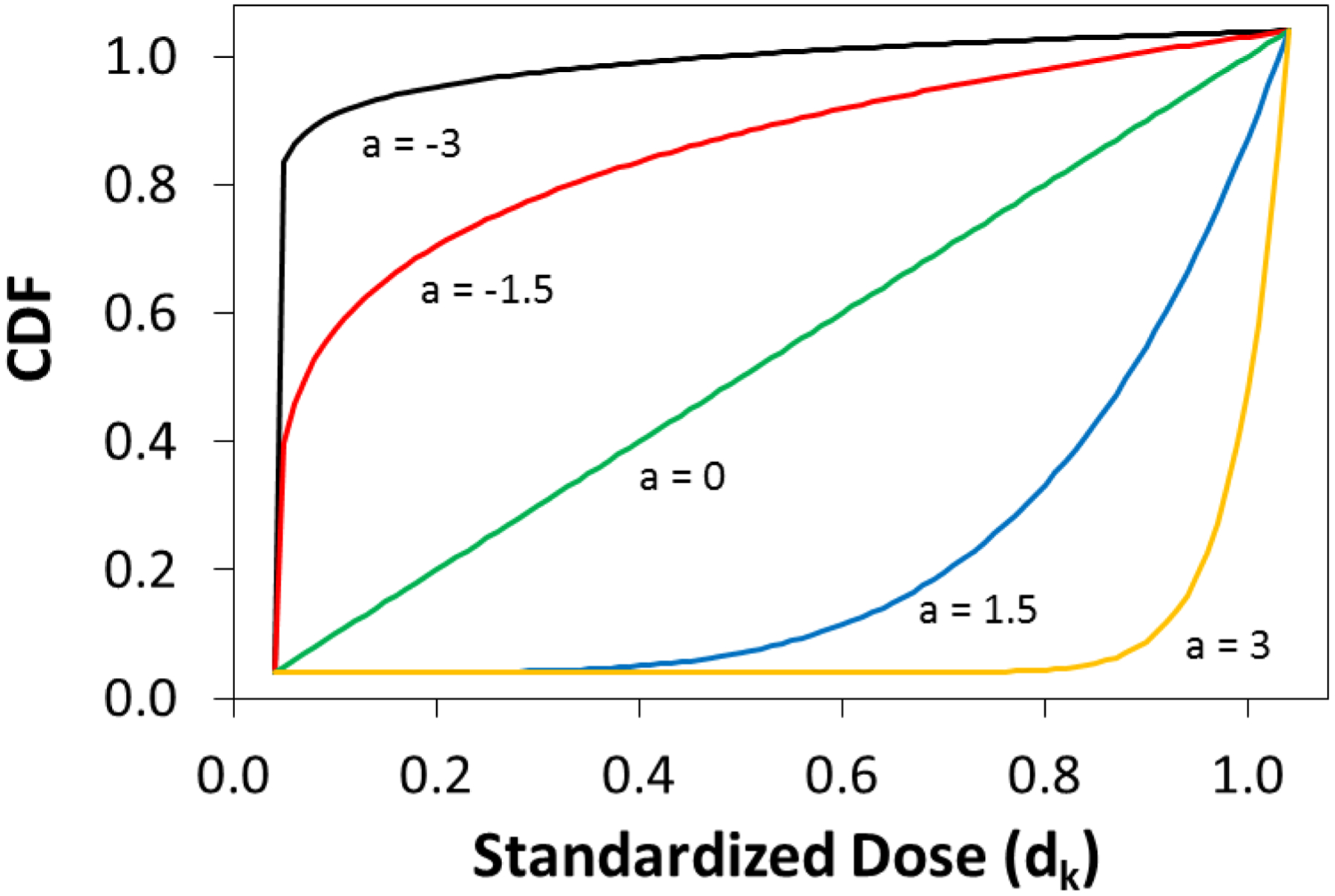
Graphical representation of the convex and concave modeling produced by the power function.
An important feature of the proposed approach for calculating a scalar from a GPS vector is its compatibility with any parametric or machine learning model that produces a GPS vector. Currently, there are no methods for multinomial treatment propensity scoring that are both “propensity model-free” and that produce a scalar balancing score to enable matching and stratification. While it may initially appear that other methods (e.g. multivariate distances, Kolmogorov-Smirnov test statistic, isotonic regression, Kullback–Leibler divergence, etc.) could be used to differentiate CDFs derived from the GPS vector, these methods do not result in a scalar balancing score. Although these alternative options may be used to match subjects, they do not allow for stratification. The proposed approach in equation (4) will both accurately describe the curvature of the CDF and also produce a single scalar balancing score that can easily be used for both matching and stratification of subjects.
Unlike ordinal treatment settings where there is a natural ordering to the treatments, multinomial treatments can be aligned in any order within the GPS vector. In a setting with three multinomial treatments (A, B, and C), for example, the GPS vector can be ordered as A-B-C, A-C-B, B-A-C, B-C-A, C-A-B, and C-B-A. Each ordering is intuitive and will produce a different CDF, and subsequently a new shape parameter, ã, for each subject, potentially leading subjects to be matched or stratified differently depending on which ordering of the GPS vector is selected. Since a balancing score is just a function of covariates such that the conditional distribution of the covariates given the balancing score is the same for all treatments,9 for three multinomial treatments, there are 6 different balancing scores produced by the proposed GPS-CDF method. By rearranging the GPS vector for all possible orderings, K! balancing scores can be created in a K treatment setting. As with standard propensity score methods, covariate balance can be assessed after matching or stratification based on each of the K! orderings of the GPS vector to choose the ordering and method that creates the best covariate balance in the data. While this may at first appear ad hoc, it has a precedent in the literature - several recently proposed propensity score methods seek to optimize covariate balance before conducting outcome analyses.43,50,51 For example, the spatial propensity score method proposed by Papadogeorgou et al. incorporates an automated data-driven process of selecting matched pairs over a possible range of weights, and further selects the weight that achieves the best covariate balance.51 In this way, the proposed iterative nature of finding the ã that optimizes covariate balance is analogous to the aforementioned method. Covariate balance should be assessed using each resultant K! balancing score produced by the GPS-CDF method, and the ordering that achieves the best covariate balance, among all subjects, should be retained for the outcome analysis.
2.1. GPS-CDF Matching
The proposed metric for matching is the absolute difference between the power parameters for two subjects, ãi and ãj who received different treatments. Minimizing this difference will jointly match subjects with similar values of ã while ensuring the subjects received different treatments. This metric for two subjects, i and j, is given by equation (6).
| (6) |
As the estimated power parameter, ã, is a scalar value, it can be used to create either matched pairs or matched sets (which contain one subject from each treatment group) using either greedy or optimal matching algorithms, as chosen by the investigator. Briefly, greedy matching creates matches using the best available subjects (based on the metric given by equation (6)) and then removes them from the pool of potential matches, whereas optimal matching makes selections in order to minimize the total distance among all possible matches.52,53 Several matching algorithms have been proposed for multinomial treatments17,21,23,24,29,30,54; therefore, the choice of matching algorithm will ultimately be determined by the causal estimate of interest. For example, when ATT is of interest, a reference treatment group is selected and all subjects within the reference group are matched to all other treatments.17,23 Subjects receiving the reference treatment who were matched to subjects receiving all other treatments are combined and taken as the matched sets.17,23 If ATE is of interest, one possible method is to create matched pairs for each pairwise treatment comparison. An alternative method is to create all potential matched set combinations, and those sets which minimize the ã distance between matches can be selected to form the final matched cohort.
After the selected matching procedure is performed for each of the K! orderings of the GPS vector, the order that creates matches with the best covariate balance is retained for the outcome analysis. As is standard with propensity score methods, we propose selecting the ordering that minimizes the standardized mean difference (SMD) within matches.16,17,19,30,37,43,50,51 Formally, this selection can be written as:
| (7) |
where ãk is the ã derived from each K! ordering of the GPS vector, P is the number of covariates, is the index for the number of matched pair treatment groups created from each ordering of the GPS vector, and ti = 1,2, …, K represents the multinomial treatments. The following steps detail the matching procedure:
Choose variables related to the treatments to include in the propensity model (see Brookhart et al. for a detailed discussion of variable selection for propensity models).55
Estimate the GPS vector for each subject using any desired parametric or machine learning model (i.e. multinomial logistic regression, GBM, etc.).
Choose an ordering of the K treatments within the GPS vector.
Calculate the CDF of the ordered GPS vector for each subject.
Fit a one parameter power function to the CDF of each subject to obtain ã.
Calculate the Δ(i,j) matrix between all pairs of subjects.
Create matches using an appropriate matching algorithm.
Repeat steps 3–7 for each additional (K! − 1) ordering of the GPS vector.
Assess covariate balance after matching separately for each of the K! balancing scores via SMD.
Retain the balancing score that creates matches with the best covariate balance.
Conduct a matched outcome analysis to estimate ATE or ATT (e.g. conditional logistic regression).
2.2. GPS-CDF Stratification
The method for stratification follows closely to the method proposed for matching. Using the estimated power parameter, ã, strata can be created to group subjects with similar values of ã who received different treatments. Thus within strata, there will be subjects with similar covariate distributions and multiple subjects receiving each treatment. Prior studies have shown that stratifying the data into quintiles removes approximately 90% of the initial observed covariate imbalance.10,19,31,56
As with the matching procedure, stratification can be performed for each of the K! rderings of the GPS vector. Again, the ordering that creates the strata with the best covariate balance should be retained for the outcome analysis. We propose selecting the ordering that minimizes the SMD within strata.16,17,19,30,37,43,50,51 Formally, this selection can be written as:
| (8) |
where ãk is the ã derived from each K! ordering of the GPS vector, P is the number of covariates, is the number of strata created for each ordering of the GPS vector, and ti = 1, 2, …, K represents the multinomial treatments. The following steps detail the stratification procedure:
Repeat steps 1 and 2 from the CDF matching procedure.
Choose an ordering of the K treatments within the GPS vector.
Calculate the CDF of the ordered GPS vector for each subject.
Fit a one parameter power function to the CDF of each subject to obtain ã.
Rank observations based on their value for the power parameter ã and separate the data into quintiles.
Repeat steps 3–5 for each additional (K! − 1) ordering of the GPS vector.
Assess covariate balance after stratification separately for each of the K! orderings via SMD.
Retain the GPS vector ordering that creates strata with the best covariate balance.
Conduct a stratified outcome analysis to estimate ATE or ATT (e.g. conditional logistic regression).
3. Simulation Study
A simulation study is conducted to determine how the GPS-CDF matching and stratification methods perform under different data scenarios with varying degrees of model misspecification. The design of the current simulation follows closely to several recently published simulations that seek to be representative of real data.36,44,50 Four data scenarios are considered with three treatment categories, one binary outcome, and nine baseline covariates. Six covariates are associated with treatment assignment probability, and six covariates are associated with outcome assignment probability, producing various levels of treatment and outcome confounding. A table describing the associations of the baseline covariates with the treatment and outcome variables is shown in Table 1. From the table, it can be observed that x1, x2, x4, and x5 are generated to be pretreatment confounders.
Table 1.
True association between baseline covariates with treatment and outcome. Note, x1, x2, x4, and x5 are simulated to be pretreatment confounders.
| Strongly Associated with Treatment | Moderately Associated with Treatment | Independent of Treatment | |
|---|---|---|---|
| Strongly Associated with Outcome | x1 | x2 | x3 |
| Moderately Associated with Outcome | x4 | x5 | x6 |
| Independent of Outcome | x7 | x8 | x9 |
The four data scenarios considered within this simulation study are similar to those of Fong et al. and Greene and vary whether treatment and outcome assignment models are correctly specified.36,50 Incorrect specification is created through inclusion of a non-linear term. The nine baseline covariates are multivariate normally distributed with mean 0, variance 1, and covariances of 0.2.
Scenario 1 assumes both the treatment and outcome models are correct through inclusion of only linear terms. The true treatment and outcome models are given by equations (9) and (10), respectively.
| (9) |
| (10) |
The three-level multinomial treatment and binary outcome variables are simulated by sampling one value from a multinomial distribution and Bernoulli distribution using the probabilities calculated from equation (9) and (10), respectively, as the probability sampling weights. From the data generating procedure, the true treatment effects are 0.7, 0.4, and −0.3 for treatment pairs (1, 2), (1, 3), and (2, 3), respectively.
Scenario 2 introduces a non-linear term based on a mis-measured variable, (xi,1 + 0.5)2, into the treatment assignment model, while the outcome model remains the same as equation (10). The misspecified treatment model is given by:
| (11) |
Scenario 3 introduces a non-linear term based on a mis-measured variable, (xi,1 + 0.5)2, into the outcome assignment model, while the treatment model remains the same as equation (9). The misspecified outcome model is given by:
| (12) |
Finally in Scenario 4, both the treatment and outcome models are misspecified using the treatment and outcome assignment models detailed in equations (11) and (12).
4. Results
For each data scenario considered, 1,000 datasets each containing 1,000 observations are generated. Five analytic tools are used to estimate and compare the conditional ATEs (log ORs)18: unadjusted (crude odds ratio) model, adjusted (adjusted odds ratio) model, GBM with IPTW, GPS-CDF greedy matching, and GPS-CDF stratification. The GBM propensity model adjusts for all nine baseline covariates. Additionally, the GPS vector generated through GBM is used for GPS-CDF matching and stratification, and a caliper of 0.25 standard deviations of ã is used for GPS-CDF greedy matching.57,58 Outcome models to obtain conditional ATE estimates utilize logistic regression for the unadjusted and adjusted models, survey-weighted generalized linear models for GBM weighting, and conditional logistic regression for GPS-CDF matching and stratification. Furthermore, outcome models (with the exception of the unadjusted model) adjust for all first order covariates associated with outcome assignment.10,13,18,42
Figure 2 is a graphical depiction of the degree of covariate balance achieved by each analytical tool under both the correctly and incorrectly specified treatment model in terms of maximum pairwise SMDs for each of the nine baseline covariates within each simulated data set.17 Methods that achieve covariate balance would have smaller maximum SMD values. The three propensity scoring methods achieve better covariate balance, on average, versus the unadjusted analysis. Within the correctly specified treatment model (left plot), GBM weighting produces better balance than both GPS-CDF matching and stratification. GPS-CDF matching and stratification produce similar balance in the correctly specified treatment model, but it appears that GPS-CDF stratification produces fewer outliers. Within the incorrectly specified treatment model (right plot), GBM weighting and GPS-CDF matching produce similar balance results. GPS-CDF stratification produces slightly worse balance than GBM weighting and GPS-CDF matching, but still produces better balance than the original data.
Figure 2.

Graphical representation of the covariate balance achieved by each method under the correctly specified and incorrectly specified treatment assignment models. SMD was calculated for all baseline covariates within each treatment pair, and the maximum SMD across treatment pairs was retained.
For each of the data scenarios considered, the five analysis methods are compared using average bias, mean squared error (MSE), and coverage probability of the estimated conditional treatment effects. As there are three treatments, the performance of each method is assessed for each of the three conditional ATEs. Figure 3 shows the distribution of the conditional ATE estimates from each analytical method under each data scenario between treatment 1 and treatment 3. The true pairwise treatment effect of 0.4 is included as the dotted horizontal line.
Figure 3.

Distribution of the conditional ATE estimates for each method under each scenario between treatment 1 and treatment 3. The true effect value of 0.4 is included as the dotted horizontal line.
Within Scenario 1, all methods produce estimates with minimal bias and high coverage probabilities, with the exception of the unadjusted model. The adjusted model, which does not include any propensity scoring, actually has the smallest MSE compared to the methods that include propensity models. This result was anticipated since there is no misspecification in either the treatment or outcome model under this data scenario. Additionally, GBM weighting performs better in terms of bias and MSE compared to GPS-CDF matching. However, even though GBM weighting produces better balance than GPS-CDF stratification, as indicated in Figure 2, GPS-CDF stratification has lower bias and higher coverage probability compared to GBM weighting. In Scenario 2, where the treatment model is misspecified, but the outcome model is correct (Figure 3, Scenario 2), results are consistent with Scenario 1. Again, GPS-CDF stratification produces lower bias than all other methods and obtained coverage probability closest to the nominal 95%.
For Scenario 3, which includes a correctly specified treatment model but misspecified outcome model (Figure 3, Scenario 3), GPS-CDF matching and stratification have lower bias compared to all other methods, with both GPS-CDF methods outperforming GBM weighting in terms of coverage probability. Finally, in Scenario 4 (Figure 3 Scenario 4), the adjusted model, GBM weighting, and GPS-CDF matching all fail to obtain accurate treatment estimates. GPS-CDF stratification is still able to produce minimally biased conditional ATE estimates while maintaining low MSE and coverage probability close to 0.9 when both the treatment and outcome models are misspecified.
The conditional ATEs for the comparisons between treatments 1 and 2 (Supplemental Figure 1) and between treatments 2 and 3 (Supplemental Figure 2) are consistent with those detailed above. GPS-CDF stratification produces estimates with minimal bias and MSE, while maintaining high coverage probability across all data scenarios. An additional big data simulation (Appendix) further demonstrates the utility of the GPS-CDF method, compared to IPTW, when applied to data with a larger covariate space. In this large covariate setting, GPS-CDF matching outperforms all other comparison methods in terms of bias, MSE, and coverage probability. Analogous to the aforementioned simulation study, IPTW produces severally biased conditional ATE estimates when analyses include a large covariate space.
Finally, the accuracy of the CDF mapping produced by the GPS-CDF method for 3, 4, 6, and 10 treatments is tested (Supplemental Figure 3). For each multinomial treatment group, 1,000 subjects are simulated in a manner similar to the above simulation study, GBM is used to estimate the GPS vector for each simulated subject, and the subsequent CDF vector for each subject is found by summing across the subject specific GPS vectors, and ã is estimated. Overall, as the number of treatment groups increase, the power function still accurately maps the CDF of the GPS vector. The average of the absolute difference between the CDF of the GPS vector and the produced power function is 0.034, 0.047, 0.049, and 0.055 for 3, 4, 6, and 10 treatments, respectively, averaging across simulated subjects.
5. Data Application: Effect of vasopressor choice on mortality in patients with aneurysmal subarachnoid hemorrhage from Cerner Health Facts EHR database
Subarachnoid hemorrhage (SAH) is defined as a blood vessel that bursts in the brain and is a devastating cerebrovascular condition not only due to the effect of the hemorrhage but also the complicated treatment regimens required to manage such patients. A major complication resulting from SAH includes delayed cerebral ischemia (DCI), which is a main source of morbidity following SAH.59 Although current guidelines suggest maintaining an elevated blood pressure after management of an aneurysm may reduce the incidence of DCI, there is little data to suggest which vasopressor is the most efficacious to achieving this end with regards to mortality. The effectiveness of the three most commonly accepted drugs used to achieve an increase in blood pressure (dopamine, phenylephrine, and norepinephrine) are studied in relation to mortality in patients with non-traumatic SAH.
The study population included in the current analysis has been previously described.60 Briefly, the Cerner Health Facts EHR database was queried from years 2000 to 2015 to select adult patients (over age 17) with a new diagnosis of aneurysmal SAH based on ICD-9 code 430. Only patients who received infusions of dopamine, phenylephrine, or norepinephrine were included in the study population.60 Among the 4,850 patients that met the above study inclusion criteria, 40 patients presented with multiple first vasopressor treatments; these patients were excluded from the cohort. Furthermore, patients whose diagnosis included a traumatic cause of SAH (based on ICD 9 codes: 800.2x, 800.7x, 801.2x, 801.7x, 803.2x, 803.7x, 804.2x, 804.7x, 852.x) or with unknown mortality status were excluded from the study population leaving 2,634 patients in the final cohort.
The propensity score analysis presented here includes 2,417 patients with complete data for demographic variables (age, gender, race, and marital status) as well as pretreatment medication variables. Of the patients included in the analysis, 492, 1,253, and 672 were administered dopamine, phenylephrine, and norepinephrine, respectively. In total, 170 pretreatment variables are entered into GBM in order to produce patient specific GPS vectors (Supplemental Table 1). More details on variable selection as well as variables included in the propensity model can be found in previous work.60
The five analytical methods investigated in Sections 3–4 are applied to determine the causal relationship between vasopressor choice and mortality. A visual representation of the covariate balance achieved by each method is depicted in Figure 4. The left plot shows maximum pairwise SMD for each potential pretreatment confounder. Similarly, the right plot shows the average pairwise SMD, which is calculated by averaging the SMD for each potential pretreatment confounder across treatment pairs. It has been suggested that values of SMD less than 0.2 indicate small levels of covariate imbalance.16,61 Based on this cutoff, both GBM weighting and GPS-CDF matching produce better covariate balance compared to the original data, while GPS-CDF stratification produces less satisfactory covariate balance.
Figure 4.

Graphical representation of the covariate balance achieved by each method for SAH patients within the Cerner Health Facts EHR database. The left plot presents the maximum pairwise SMD across treatment groups for each potential confounder. The right plot presents the average pairwise SMD across treatment groups for each potential confounder.
As all subjects were eligible for all three treatments, conditional ATE is the estimand of interest. Results from applying each of the five analytic methods assessed in Sections 3–4 are shown in Table 2. Both GPS-CDF matching and stratification show that the odds of mortality are significantly higher in patients who received dopamine versus patients who received phenylephrine (ORGPS-CDF Matching = 1.53, 95% CI [1.11, 2.10], p = 0.008; ORGPS-CDF Stratification = 2.59, 95% CI [2.03, 3.31], p = <0.001). Patients receiving norepinephrine have a higher odds of mortality versus those receiving phenylephrine when analyses are conducted using the GPS-CDF stratification method (ORGPS-CDF Stratification = 3.21, 95% CI [2.55, 3.31], p = <0.001), but this association is not significant with GPS-CDF matching (ORGPS-CDF Matching = 1.41, 95% CI [1.00, 1.99], p = 0.051). Furthermore, GPS-CDF matching and stratification do not show any significant differences in the odds of mortality between patients who received dopamine versus those who received norepinephrine.
Table 2.
Model estimates after applying each analytical method to SAH patients to determine the association between vasopressor and mortality within the EHR dataset. Outcome models (with the exception of the unadjusted model) adjusted for age at baseline, gender, race, and marital status.
| Analytical Method | Dopamine vs Phenylephrine | Norepinephrine vs Phenylephrine | Dopamine vs Norepinephrine | |||
|---|---|---|---|---|---|---|
| OR [95% CI] | p-value | OR [95% CI] | p-value | OR [95% CI] | p-value | |
| Unadjusted | 3.06 [2.46–3.81] | <0.001 | 2.53 [2.08–3.09] | <0.001 | 1.21 [0.96–1.53] | 0.110 |
| Adjusted | 3.02 [2.42–3.76] | <0.001 | 2.63 [2.15–3.22] | <0.001 | 1.15 [0.91–1.45] | 0.253 |
| GBM Weighted | 2.19 [1.70–2.81] | <0.001 | 2.24 [1.80–2.80] | <0.001 | 0.97 [0.75–1.27] | 0.852 |
| GPS-CDF Greedy Matched | 1.53 [1.11–2.10] | 0.008 | 1.41 [1.00–1.99] | 0.051 | 1.09 [0.79–1.49] | 0.610 |
| GPS-CDF Stratification | 2.59 [2.03–3.31] | <0.001 | 3.21 [2.55–3.31] | <0.001 | 0.81 [0.61–1.07] | 0.138 |
Importantly, all three propensity scoring approaches applied attenuate the unadjusted and covariate adjusted association between vasopressor choice and mortality. Overall, it does appear that phenylephrine is superior to dopamine with respect to mortality in patients with non-traumatic SAH, but the comparison between phenylephrine and norepinephrine remains unclear. GPS-CDF matching creates satisfactory levels of covariate balance within the data and further attenuates the association between vasopressor choice and mortality. For this analysis, the GPS-CDF approach is computationally quick; results were available in 8 minutes using a dual-core Intel Core i3–3110M with 4 GB RAM.
6. Discussion
Few existing methods for multinomial treatments propensity scoring have the capability and flexibility to estimate both ATE and ATT and correctly model data sources that present with large covariate spaces.17,21,22,24–31 Recently, researchers have advocated for the use of machine learning propensity models to produce more accurate GPS vectors especially in the presence of a large covariate space.1,39,62 Although the benefits of using GBM and other machine learning methods, are apparent, there are drawbacks to these methods that need to be addressed. Currently, the GPS vector produced by machine learning methods can only be adjusted in outcome analysis via IPTW. Although IPTW is an easily adaptable method in order to produce causal treatment effect estimates, Rubin suggested that weighting directly on the propensity score leads to a higher degree of sensitivity to model misspecification.45 Furthermore, via simulation, Yang et al. showed that when presented with six treatments (not an impossibly large number when considering EHR-derived studies), implementation of the GPS via IPTW leads to extreme weights.30 For example, the maximum weights reported by Yang et al. were 95.8 within in a three treatment scenario and 185.1 within a six treatment scenario.30 Although these extreme weights may not adversely impact covariate balance, they will lead to inaccurate ATEs/ATTs. Given the substantial limitations for IPTW for multiple treatments propensity scoring, this current paper derived and tested via simulation and practice, a novel multinomial propensity scoring technique that utilizes the entire GPS vector that can be used with matching and stratification to produce ATEs or ATTs. As the GPS-CDF method generates K! balancing scores, it follows closely to the current opinion in the literature regarding the ‘covariate balancing propensity score’43,50 and the ‘distance adjusted propensity score’.51
While other methods may be used to map CDFs (e.g. Kolmogorov-Smirnov test statistic, isotonic regression, Kullback–Leibler divergence, etc.), they do not result in a scalar balancing score that is analogous in spirit to that typically utilized in binary treatment propensity scoring. For example, the Kolmogorov-Smirnov test statistic tests the equality of CDFs through a distance-based metric.63 Although this approach may be used to match subjects with similar CDFs, the resultant pairwise distances cannot be used to easily stratify subjects. Furthermore, other common one parameter functions (e.g. exponential, logarithmic, sigmoid) do not have the same flexibility as the power function for mapping CDFs that present with both concave and convex shapes. The proposed method appears superior in addressing these limitations.
The current simulation study closely followed several recently published simulations36,44,50; matching and stratification via the GPS-CDF method produced better covariate balance than the original data in both the correctly and incorrectly specified treatment model. Although GBM weighting produced better covariate balance compared to GPS-CDF matching and stratification within the correctly specified treatment model, similar to results presented by Fong et al., this increased balance did not translate to more accurate conditional ATE estimates.50 Generalized boosted model weighting produced highly biased estimates compared to GPS-CDF stratification for each treatment comparison when both the treatment and outcome models were misspecified.
Unlike IPTW which has been shown to produce extreme weights and unreliable causal estimates as the number of multinomial treatments increase,30 the GPS-CDF method was still able to accurately map CDFs of the GPS even in the presence of numerous treatment groups. Data simulated under different multinomial treatment group scenarios, 3, 4, 6, and 10 treatments, showed that the average difference between the true CDF of the GPS vector and the estimated power function remains minimal. Thus, the GPS-CDF method can be used for any number of multinomial treatment groups, which will resolve the dimensionality issues known to arise with IPTW. Therefore, the GPS-CDF method may produce more accurate ATE and ATT estimates compared to those derived by IPTW, especially in the presence of multiple treatments.
The performance and utility of the GPS-CDF method was further demonstrated using an EHR data application. Overall, the novel multinomial propensity analysis approach, GPS-CDF, had low computational burden and produced better covariate balance compared to the unadjusted data when applied via matching. The EHR data example also demonstrated the easy applicability of the GPS-CDF approach.
There are limitations of this study. First, the EHR data application was derived from the Cerner Health Facts database, which contained a large number of patients with incomplete covariate data. Patients were included in the analysis based on a new diagnosis of SAH, but their diagnosis could not be confirmed via imaging. Furthermore, due to the absence of baseline diagnostic variables, there is of course the possibility of unmeasured confounding within the analysis, as with any propensity score analysis, especially one derived from EHR.
The GPS-CDF method presented here gives researchers more options when conducting multinomial treatment propensity scoring. This novel method can be used in conjunction with current machine learning methods in order to better facilitate propensity scoring in the presence of big data. Future studies should further evaluate the use of the GPS-CDF method when conducting propensity scoring with multinomial treatments in the context of relevant research questions. Open-source software is available to help facilitate the use of the proposed method in practice.46
Supplementary Material
Acknowledgment
This project was partially supported by the Center for Big Data in Health Sciences (CBD-HS) at School of Public Health, University of Texas Health Science Center at Houston (UTHealth), and the data extraction and preparation were partially supported by the SBMI Data Service Office and Data Science and Informatics Core for Cancer Research (funded by CPRIT RP170668) at UTHealth. The authors also acknowledge the contributions from all other members of the EHR Working Group at the CBD-HS for data cleaning and data preparation. Two authors were supported by the NIH training grant T32 GM074902.
This work was additionally supported by the Intramural Research Program of the US National Cancer Institute.
Footnotes
Data Availability
The data that support the findings of this study are available on request from the corresponding author. The data are not publicly available due to privacy or ethical restrictions.
References
- 1.Chen KP, Moskowitz A. Comparative Effectiveness: Propensity Score Analysis In: Secondary Analysis of Electronic Health Records. Cham: Springer International Publishing; 2016:339–349. [PubMed] [Google Scholar]
- 2.Patorno E, Glynn RJ, Hernandez-Diaz S, Liu J, Schneeweiss S. Studies with many covariates and few outcomes: selecting covariates and implementing propensity-score-based confounding adjustments. Epidemiology. 2014;25(2):268–278. [DOI] [PubMed] [Google Scholar]
- 3.Ju C, Combs M, Lendle SD, et al. Propensity score prediction for electronic healthcare databases using super learner and high-dimensional propensity score methods. Journal of Applied Statistics. 2019:1–21. [DOI] [PMC free article] [PubMed] [Google Scholar]
- 4.Low YS, Gallego B, Shah NH. Comparing high-dimensional confounder control methods for rapid cohort studies from electronic health records. Journal of comparative effectiveness research. 2016;5(2):179–192. [DOI] [PMC free article] [PubMed] [Google Scholar]
- 5.Schneeweiss S, Rassen JA, Glynn RJ, Avorn J, Mogun H, Brookhart MA. High-dimensional propensity score adjustment in studies of treatment effects using health care claims data. Epidemiology. 2009;20(4):512–522. [DOI] [PMC free article] [PubMed] [Google Scholar]
- 6.Schuemie MJ, Coloma PM, Straatman H, et al. Using electronic health care records for drug safety signal detection: a comparative evaluation of statistical methods. Medical care. 2012;50(10):890–897. [DOI] [PubMed] [Google Scholar]
- 7.Stuart EA, DuGoff E, Abrams M, Salkever D, Steinwachs D. Estimating causal effects in observational studies using Electronic Health Data: Challenges and (some) solutions EGEMS (Washington, DC: ). 2013;1(3). [DOI] [PMC free article] [PubMed] [Google Scholar]
- 8.Gutman R, Rubin DB. Estimation of causal effects of binary treatments in unconfounded studies. Statistics in medicine. 2015;34(26):3381–3398. [DOI] [PMC free article] [PubMed] [Google Scholar]
- 9.Rosenbaum PR, Rubin DB. The Central Role of the Propensity Score in Observational Studies for Causal Effects. Biometrika. 1983;70(1):41–55. [Google Scholar]
- 10.Rosenbaum PR, Rubin DB. Reducing bias in observational studies using subclassification on the propensity score. Journal of the American statistical Association. 1984;79(387):516–524. [Google Scholar]
- 11.Rosenbaum PR, Rubin DB. Constructing a control group using multivariate matched sampling methods that incorporate the propensity score. The American Statistician. 1985;39(1):33–38. [Google Scholar]
- 12.Stuart EA. Matching methods for causal inference: A review and a look forward. Statistical science: a review journal of the Institute of Mathematical Statistics. 2010;25(1):1. [DOI] [PMC free article] [PubMed] [Google Scholar]
- 13.Imai K, Van Dyk DA. Causal inference with general treatment regimes: Generalizing the propensity score. Journal of the American Statistical Association. 2004;99(467):854–866. [Google Scholar]
- 14.Imbens GW. The role of the propensity score in estimating dose-response functions. Biometrika. 2000;87(3):706–710. [Google Scholar]
- 15.Joffe MM, Rosenbaum PR. Invited commentary: propensity scores. American journal of epidemiology. 1999;150(4):327–333. [DOI] [PubMed] [Google Scholar]
- 16.McCaffrey DF, Griffin BA, Almirall D, Slaughter ME, Ramchand R, Burgette LF. A tutorial on propensity score estimation for multiple treatments using generalized boosted models. Statistics in medicine 2013;32(19):3388–3414. [DOI] [PMC free article] [PubMed] [Google Scholar]
- 17.Lopez MJ, Gutman R. Estimation of causal effects with multiple treatments: a review and new ideas. Statistical Science. 2017;32(3):432–454. [Google Scholar]
- 18.Abrevaya J, Hsu Y-C, Lieli RP. Estimating Conditional Average Treatment Effects. Journal of Business & Economic Statistics 2015;33(4):485–505. [Google Scholar]
- 19.Austin PC. An introduction to propensity score methods for reducing the effects of confounding in observational studies. Multivariate behavioral research. 2011;46(3):399–424. [DOI] [PMC free article] [PubMed] [Google Scholar]
- 20.Austin PC, Stuart EA. Estimating the effect of treatment on binary outcomes using full matching on the propensity score. Statistical methods in medical research. 2017;26(6):2505–2525. [DOI] [PMC free article] [PubMed] [Google Scholar]
- 21.Rassen JA, Shelat AA, Franklin JM, Glynn RJ, Solomon DH, Schneeweiss S. Matching by propensity score in cohort studies with three treatment groups. Epidemiology. 2013;24(3):401–409. [DOI] [PubMed] [Google Scholar]
- 22.Rubin DB. Using multivariate matched sampling and regression adjustment to control bias in observational studies. Journal of the American Statistical Association. 1979;74(366a):318–328. [Google Scholar]
- 23.Scotina AD, Gutman R. Matching algorithms for causal inference with multiple treatments. Statistics in medicine. 2019;38(17):3139–3167. [DOI] [PubMed] [Google Scholar]
- 24.Seya H, Yoshida T. Propensity score matching for multiple treatment levels: A CODA-based contribution. arXiv preprint arXiv:171008558 2017. [Google Scholar]
- 25.Zhao Z Using matching to estimate treatment effects: Data requirements, matching metrics, and Monte Carlo evidence. review of economics and statistics. 2004;86(1):91–107. [Google Scholar]
- 26.Tu C, Jiao S, Koh WY. Comparison of clustering algorithms on generalized propensity score in observational studies: a simulation study. Journal of Statistical Computation and Simulation. 2013;83(12):2206–2218. [Google Scholar]
- 27.Feng P, Zhou XH, Zou QM, Fan MY, Li XS. Generalized propensity score for estimating the average treatment effect of multiple treatments. Statistics in medicine. 2012;31(7):681–697. [DOI] [PubMed] [Google Scholar]
- 28.Huang I-C, Frangakis C, Dominici F, Diette GB, Wu AW. Application of a propensity score approach for risk adjustment in profiling multiple physician groups on asthma care. Health services research. 2005;40(1):253–278. [DOI] [PMC free article] [PubMed] [Google Scholar]
- 29.Lechner M Identification and estimation of causal effects of multiple treatments under the conditional independence assumption In: Econometric evaluation of labour market policies. Springer; 2001:43–58. [Google Scholar]
- 30.Yang S, Imbens GW, Cui Z, Faries DE, Kadziola Z. Propensity score matching and subclassification in observational studies with multi‐level treatments. Biometrics. 2016;72(4):1055–1065. [DOI] [PubMed] [Google Scholar]
- 31.Zanutto E, Lu B, Hornik R. Using propensity score subclassification for multiple treatment doses to evaluate a national antidrug media campaign. Journal of Educational and Behavioral Statistics. 2005;30(1):59–73. [Google Scholar]
- 32.Gu XS, Rosenbaum PR. Comparison of multivariate matching methods: Structures, distances, and algorithms. Journal of Computational and Graphical Statistics. 1993;2(4):405–420. [Google Scholar]
- 33.Hade EM, Lu B. Bias associated with using the estimated propensity score as a regression covariate. Statistics in medicine. 2014;33(1):74–87. [DOI] [PMC free article] [PubMed] [Google Scholar]
- 34.Dehejia RH, Wahba S. Causal effects in nonexperimental studies: Reevaluating the evaluation of training programs. Journal of the American statistical Association. 1999;94(448):1053–1062. [Google Scholar]
- 35.Dehejia RH, Wahba S. Propensity score-matching methods for nonexperimental causal studies. Review of Economics and statistics. 2002;84(1):151–161. [Google Scholar]
- 36.Greene Thomas J, Utilizing Propensity Score Methods for Ordinal Treatments and Prehospital Trauma Studies. Texas Medical Center Dissertations (via ProQuest). 2017. [Google Scholar]
- 37.Burgette L, Griffin BA, McCaffrey D. Propensity scores for multiple treatments: A tutorial for the mnps function in the twang package. R package Rand Corporation 2017. [Google Scholar]
- 38.McCaffrey DF, Ridgeway G, Morral AR. Propensity score estimation with boosted regression for evaluating causal effects in observational studies. Psychological methods. 2004;9(4):403. [DOI] [PubMed] [Google Scholar]
- 39.Setoguchi S, Schneeweiss S, Brookhart MA, Glynn RJ, Cook EF. Evaluating uses of data mining techniques in propensity score estimation: a simulation study. Pharmacoepidemiology and drug safety. 2008;17(6):546–555. [DOI] [PMC free article] [PubMed] [Google Scholar]
- 40.Busso M, DiNardo J, McCrary J. New evidence on the finite sample properties of propensity score reweighting and matching estimators. Review of Economics and Statistics. 2014;96(5):885–897. [Google Scholar]
- 41.Li F, Morgan KL, Zaslavsky AM. Balancing covariates via propensity score weighting. Journal of the American Statistical Association. 2018;113(521):390–400. [Google Scholar]
- 42.Hirano K, Imbens GW. Estimation of causal effects using propensity score weighting: An application to data on right heart catheterization. Health Services and Outcomes research methodology. 2001;2(3–4):259–278. [Google Scholar]
- 43.Imai K, Ratkovic M. Covariate balancing propensity score. Journal of the Royal Statistical Society: Series B (Statistical Methodology). 2014;76(1):243–263. [Google Scholar]
- 44.Austin PC, Grootendorst P, Anderson GM. A comparison of the ability of different propensity score models to balance measured variables between treated and untreated subjects: a Monte Carlo study. Statistics in medicine. 2007;26(4):734–753. [DOI] [PubMed] [Google Scholar]
- 45.Rubin DB. On principles for modeling propensity scores in medical research. Pharmacoepidemiology and drug safety. 2004;13(12):855–857. [DOI] [PubMed] [Google Scholar]
- 46.Brown DW, Greene TJ, DeSantis SM. GPSCDF: Generalized Propensity Score Cumulative Distribution Function. R Package. Rand Corporation 2019. [Google Scholar]
- 47.O’Quigley J, Pepe M, Fisher L. Continual reassessment method: a practical design for phase 1 clinical trials in cancer. Biometrics. 1990;46(1):33–48. [PubMed] [Google Scholar]
- 48.Storer BE. Design and analysis of phase I clinical trials. Biometrics. 1989;45(3):925–937. [PubMed] [Google Scholar]
- 49.Marquardt DW. An algorithm for least-squares estimation of nonlinear parameters. Journal of the society for Industrial and Applied Mathematics. 1963;11(2):431–441. [Google Scholar]
- 50.Fong C, Hazlett C, Imai K. Covariate balancing propensity score for a continuous treatment: Application to the efficacy of political advertisements. The Annals of Applied Statistics. 2018;12(1):156–177. [Google Scholar]
- 51.Papadogeorgou G, Choirat C, Zigler CM. Adjusting for unmeasured spatial confounding with distance adjusted propensity score matching Biostatistics (Oxford, England: ). 2018. [DOI] [PMC free article] [PubMed] [Google Scholar]
- 52.Lu B, Greevy R, Xu X, Beck C. Optimal nonbipartite matching and its statistical applications. The American Statistician. 2011;65(1):21–30. [DOI] [PMC free article] [PubMed] [Google Scholar]
- 53.Guo S, Fraser MW. Propensity score analysis. Sage; 2015. [Google Scholar]
- 54.Imbens GW, Rubin DB. Causal inference in statistics, social, and biomedical sciences. Cambridge University Press; 2015. [Google Scholar]
- 55.Brookhart MA, Schneeweiss S, Rothman KJ, Glynn RJ, Avorn J, Stürmer T. Variable selection for propensity score models. American journal of epidemiology. 2006;163(12):1149–1156. [DOI] [PMC free article] [PubMed] [Google Scholar]
- 56.Cochran WG. The effectiveness of adjustment by subclassification in removing bias in observational studies. Biometrics. 1968:295–313. [PubMed] [Google Scholar]
- 57.Cochran WG, Rubin DB. Controlling Bias in Observational Studies: A Review. Sankhyā: The Indian Journal of Statistics, Series A (1961–2002) 1973;35(4):417–446. [Google Scholar]
- 58.Lunt M Selecting an Appropriate Caliper Can Be Essential for Achieving Good Balance With Propensity Score Matching. American Journal of Epidemiology. 2014;179(2):226–235. [DOI] [PMC free article] [PubMed] [Google Scholar]
- 59.Roy B, McCullough LD, Dhar R, Grady J, Wang Y-B, Brown RJ. Comparison of initial vasopressors used for delayed cerebral ischemia after aneurysmal subarachnoid hemorrhage. Cerebrovascular Diseases. 2017;43(5–6):266–271. [DOI] [PubMed] [Google Scholar]
- 60.Williams G, Maroufy V, Rasmy L, Brown D, Yu D, Zhu H, Talebi Y, Wang X, Thomas E, Zhu G, Yaseen A, Miao H, Novelo L, Zhi D, DeSantis S, Zhu H, Yamal JM, Aguilar D, Wu H Vasopressor Treatment and Mortality Following Non-Traumatic Subarachnoid Hemorrhage: A Nationwide EHR Analysis Neurosurgical Focus. 2020; in press. [DOI] [PubMed] [Google Scholar]
- 61.Cohen J Statistical power analysis for the behavioral sciences. Hillsdale NJ: L. Erlbaum Associates; 1988. [Google Scholar]
- 62.Guertin JR, Rahme E, Dormuth CR, LeLorier J. Head to head comparison of the propensity score and the high-dimensional propensity score matching methods. BMC medical research methodology. 2016;16:22. [DOI] [PMC free article] [PubMed] [Google Scholar]
- 63.Massey FJ. The Kolmogorov-Smirnov Test for Goodness of Fit. Journal of the American Statistical Association. 1951;46(253):68–78. [Google Scholar]
Associated Data
This section collects any data citations, data availability statements, or supplementary materials included in this article.