Detecting prostate cancer using deep learning convolution neural network with transfer learning approach

Abstract

Prostate Cancer in men has become one of the most diagnosed cancer and also one of the leading causes of death in United States of America. Radiologists cannot detect prostate cancer properly because of complexity in masses. In recent past, many prostate cancer detection techniques were developed but these could not diagnose cancer efficiently. In this research work, robust deep learning convolutional neural network (CNN) is employed, using transfer learning approach. Results are compared with various machine learning strategies (Decision Tree, SVM different kernels, Bayes). Cancer MRI database are used to train GoogleNet model and to train Machine Learning classifiers, various features such as Morphological, Entropy based, Texture, SIFT (Scale Invariant Feature Transform), and Elliptic Fourier Descriptors are extracted. For the purpose of performance evaluation, various performance measures such as specificity, sensitivity, Positive predictive value, negative predictive value, false positive rate and receive operating curve are calculated. The maximum performance was found with CNN model (GoogleNet), using Transfer learning approach. We have obtained reasonably good results with various Machine Learning Classifiers such as Decision Tree, Support Vector Machine RBF kernel and Bayes, however outstanding results were obtained by using deep learning technique.

Introduction

Prostate cancer is the most common malignancy (other than skin cancer) diagnosed in men. Prostate cancer is a disease defined by the abnormal growth of cells. These abnormal cells can proliferate in an uncontrolled way and, if left untreated, form tumors which may metastasize or spread to other parts of the body. Prostate cancer has the potential to grow and spread quickly, but for most men, it is a relatively slow growing disease. On an annual basis globally, approximately (1.1) million men are diagnosed with prostate cancer.

Recently, prostate cancer has become one of the most commonly diagnosing carcinomas among males. In 2017, Statistic of United States shows that prostate cancer is ranked first among all cancer cases in males (Siegel et al. 2017). Rapid increase in growth of prostate cancer in China is reported in a study conducted in 2015 (Chen et al. 2016). There is an estimate of (1.7) million diagnosed cases up till 2030 (Chou et al. 2011). To increase probability of prosperous treatment diagnosing of prostate cancer is crucial. In last few years diagnosed cases of prostate cancer are increased because of PSA (prostate specific antigen) testing. However, prostate cancer grow slowly and has low risk of death in nearly half of diagnosed prostate cancers (Eggener et al. 2015). Transrectal ultrasonography guided biopsy (TRUS) is standard of care for diagnosing prostate cancer. It shows high rate of incorrect results and painful procedure of diagnosing prostate cancer (Costa et al. 2015). Most cases of this type of cancer is found in aged men so a less harmful technique with accurate classification of prostate cancer is required. Radiation therapy is a technique to restrict or damage effected cells in prostate gland and Brachytherapy is the one of the oldest technique for prostate carcinoma (Talcott et al. 2014). Within recent past years one of the modern developed technique is brachytherapy for transperineally permanent prostate (Kattan et al. 2001).

In last decade, medical images creates huge impact on the process of analysing different body parts (Rathore et al. 2015). Various researchers have developed different techniques for detection and classification of prostate carcinoma. Some of techniques and tools developed in past few years to detect prostate cancer include PSA, DRE (digital rectal examination) and Transrectal ultrasonography (TRUS). It was observed that these techniques show incorrect results (Yu and Hricak 2000).

PSA technique employed by Schröder et al. (2009) has the ability to detect cancer with slow growth and diagnostic with this technique has helped in reducing the rate of death to one-fifth. On the other hand, TRUS guided biopsy method failed to diagnose all cases of prostate cancer and also its accuracy was not found good enough. Magnetic Resonance Imaging (MRI) was employed as a tool for TRUS. The MR images have capability to detect prostate carcinoma because of high quality resolution of these images (Vos et al. 2010; Wall et al. 2010). MRI has become important part of prostate carcinoma detection process. Improved classification and detection results of prostate carcinoma based on computerized tool i.e. computer power-assisted diagnosing (CAD) are employed that showed good prospect of computer based techniques for detection and characterization (Seltzer et al. 1997; Hricak et al. 2007). Capability of texture and morphology of MRI displays signature of effects of diseases. This feature of MRI helps in classification and detection of diseases (Fan et al. 2007).

In the past, researchers extracted different features from physiological and neurophysiological systems to understand the underlying dynamics. Currently researchers developed automated tools for studying the neural dynamics of the physiological signals and systems. Recently, Bonzon (2017) proposed neuro-inspired symbolic models of cognition which links the neural dynamics to behavior though asynchronous communication. Moreover, Hussain (2018) computed different features from EEG signals with epileptic seizures and applied robust machine learning techniques with parametric optimization approach and obtained higher detection performance. Likewise, Khaki-Khatibi et al. (2019) computed the relationship between the use of electronic devices and susceptibility to multiple sclerosis and obtained very highly significant results. Likewise, Bonzon (2017) proposed neuro-inspired symbolic models of cognition which links the neural dynamics to behavior though asynchronous communication. Moreover, Hussain (2018) computed different features from EEG signals with epileptic seizures and applied robust machine learning techniques with parametric optimization approach and obtained higher detection performance. Similarly, Khaki-Khatibi et al. (2019) computed the relationship between the use of electronic devices and susceptibility to multiple sclerosis and obtained very highly significant results. Hussain et al. (2018a) recently extracted texture, morphological, SIFT and EFDs features from Prostate Cancer database and used different machine learning techniques to detect the cancer and Hussain et al. (2018b) extracted the multimodal features to detect the brain tumor. Hussain et al. (2018c) applied Bayesian inference approach to compute the association among the morphological features extracted from Prostate cancer images. The performance obtained using morphological features was also improved. The purpose of this study was deeper network relationship analysis using morphological features using node and arc analysis to judge the strength of nodes.

Likewise, Hussain et al. (2018a) introduced a technique to detect prostate cancer by extracting various features from MRI such as SIFT, Morphology, EFDs, Texture and Entropy. Based on these extracted features different classifiers such as SVM, DT and Bayes were used to classify prostate cancer. By using single feature maximum accuracy of 98.34% with area under curve (AUC) of 0.999 was recorded, while highest accuracy of 99.71% with AUC of 1.00 was obtained by employing combination of feature Hussain et al. (2017). Li et al. (2018) also extracted some features and got AUC of 0.99 by employing SVM. Hinton et al. (2006) proposed greedy technique known as Restricted Boltzman Machines in which he trained layers one by one and avoids vanishing gradient problem and opens door for deeper networks. Deep learning improves classification results of computer vision (Krizhevsky et al. 2012) and speech recognition (Hinton et al. 2012). Recently, Hussain et al. (2019) extracted different features from Lung cancer imaging data and employed refined fuzzy entropy methods to quantify the dynamics of lung cancer.

Perez et al. (2016) has developed another feature extraction technique by computing features such as Local binary patterns, texture features etc. and obtained performance of 81–85% in terms of AUC. Technique proposed by (Han et al. 2008) has shown a specificity of about 90–95% by using SVM on texture and shape based features. Cameron et al. (2014) proposed a hybrid model based on morphological and textural features and got specificity of 78%. Doyle et al. (2006) obtained accuracy of 88% to detect prostate carcinoma by extracting texture features with first order statistics. Moreover, Isselmou et al. (2016) introduced a new technique to detect cancer automatically from MRI inspired by threshold segmentation based on morphological operations, and obtained an accuracy of around 95.5%. By using small convolutional kernels, Pinto et al. (2016) obtained accurate tumor segmentation of brain. Likewise, Liu et al. (2014) applied deep learning technique to detect Alzheimer’s from MRI and reported an overall accuracy of 87%. In recent years different researchers such as Mooij et al. (2018), Asvadi et al. (2018) and Zabihollahy et al. (2019) applied Deep learning based technique U-Net (Ronneberger et al. 2015) and its variants (based on CNN) to detect prostate cancer. In which encoders and decoders are used to classify healthy and no healthy pixels. The researchers Liu et al. (2019) proposed improved ResNet50 (He et al. 2016) that provides more information than these mentioned studies, but all mentioned CNN based methods requires large size of dataset and computational resources.

Previously employed techniques failed to provide higher performance because they cannot extract hidden features. Some of past proposed methods could not apply enough techniques to detect cancer. Different features extraction techniques proposed by Hussain et al. (2017) provides good results but still improvement is not enough because ML algorithms results cannot improve results by fine tuning. This problem can be answered by employing deep learning technique that allows fine tuning and are based on optimized activation function. Training of CNN network requires too much processing power and time, so in this study transfer learning approach is used by employing GoogleNet. Below figure shows general overview of proposed system in which image is taken in first step than feature extraction and classification is done by (GoogleNet) (Fig. 1).

Fig. 1.

Overview of GoogleNet method by employing transfer learning

Materials and methods

Dataset

Dataset that are used in this study are publicly available at Prostate (2018) provided by the Harvard University, Harvard medical School. Production of this dataset has been funded by National Institutes of Health (department of United State) grant. The dataset contains Medical Resonance Imaging (MRI) of 230 patients with different categories, dataset is arranged in various series and examination description. In this study, MRI of two type of cases are chosen (prostate, brachytherapy), last series of patient test are taken for classification. Last series contains MRI images of T1-Weighted scans and shows Axil plane. This database was obtained in accordance with the regulations of HIPAA and constructed with proper internal review board (IRB) approval. Moreover, production of this database was funded by NIH Grant U41RR019703. All images in the database includes those obtained T1-weighted, diffusion-weighted, and dynamic contrast material-enhanced (DCE) imaging sequence. Experienced uroradiologists reviewed the MR images who knew that the patients had undergone radical prostatectomy but were blinded to the other data. They evaluated the images obtained with the three pulse sequences concomitantly. First, all prostate lesions of the peripheral zones were noted that showed low signal intensity on T1-weighted images and or apparent diffusion coefficient (ADC) map and or that showed early enhancement on DCE images. Then all transition zone lesions were noted that showed homogenous low signal intensity on T1-weighted images, with ill-defined margins, no capsule and no cyst (Lemaitre et al. 2009; Oto et al. 2010; Chesnais et al. 2013; Akin et al. 2006). In the present study, 20 patient’s data are taken that consist of total of 682 MRI and 482 MRI from Prostate patients and 200 MRI from Brachytherapy patients are used, 70 percent images are used for training CNN (GoogleNet) network and 30% for validation and testing.

Deep learning

Deep learning is a part of machine leaning that comes out from previously methods of ML to ANN. Working of Artificial neural networks (ANN) is like a human brain. In ANN computation performed by neurons that are basic units of computation, these neurons perform some operation and forward information to other neurons to perform further operations. Layers are formed by groups of neurons, normally calculations of one layer is transferred to another layer but some networks allow to feed information within layers neurons or previous layers. Final results are output of last layer which can be used for regression and classification. Basically deep learning automatically extracts information from the data (Bengio et al. 2012; Lillicrap et al. 2015; Bengio 2013) which helps in analysis and prediction ability for the complex problems.

Hinton et al. (2006) proposed greedy technique known as Restricted Boltzman Machines in which he trained layers one by one and avoids vanishing gradient problem and opens door for deeper networks. Deep learning improves classification results of computer vision (Krizhevsky et al. 2012) and speech recognition (Hinton et al. 2012).

Convolutional neural networks

CNNs have many application such as object detection, object recognition, image segmentation, face recognition, video classification, depth estimation and image captioning (Krizhevsky et al. 2012; Girshick et al. 2012; Shelhamer et al. 2017; Taigman et al. 2014; Karpathy et al. 2014; Eigen et al. 2014; Karpathy and Li 2015). In machine vision neural network got better results by employing convolutional neural network. Then this idea inherited by researchers in industrial areas where this technology becomes popular. LeCun et al. (1998) proposed design that are improved design than (Homma et al. 1988) architecture of today’s CNN is like LeCun design. CNN becomes popular by winning the ILSVRC2012 competition (Krizhevsky et al. 2012).

Convolutional layer

The convolutional layer works with 3D objects rather than one dimensional layer. It looks like CNN use 2D images but mostly images have red, green and blue intensities which gives us 3rd dimension also known as channel. Commonly for colored images depth is 3 whereas for black-and white images the depth is 1. To find interesting features convolutional layers goes deeper and deeper in the network and increases depth. Earlier layers identify basic features like blobs, edges and colors, last layers differentiate the complicated objects such as animals, human faces because these layers include more neurons.

Filter (kernel) are included in convolutional layers. Let KN be a kernel with m rows, ñ columns and depth dt. Then receptive field (KNm × KNñ) on the image have the kernel of the size (KNm × KNñ × dt) to work with. The kernel size is smaller than size of images and then kernel produces a features map. Basically, sum of multiplication of elements of the kernel and images are convolution. But thing to remember is that dt of the input image and kernel is equal but it varies within the network. Stride is another option that are initialized before the training, it shows rate to which kernel can move at a time. Disadvantage of using stride in convolutional layers is decreased in map size output. Below equation shows connection between output ÕÛ and input size of an image îm by using convolutional along stride SD and kernel KN. Where output row size ÕÛm and column size ÕÛñ of CN (convolutional layers) are determined as follows:

$$\begin{array}{cc}\hfill \text{ O Û m}& =\text{î mm}-\text{KDmSD}+1,\hfill \\ \hfill \text{ O Û n}& =\text{î mn}-\text{KDnSD}+1\hfill \\ \hfill \end{array}$$ 1

After this layer, the network goes towards next layer may be new convolutional layer or a pooling layer.

Pooling layer

The pooling layer is down sampling layer which produces output with decreased size, and it operates independently on each depth part. Pooling layer consist of filters that moves with predetermined value of stride to give output (Goodfellow et al. 2016). There are many pooling methods such as max pooling, average pooling, L2-norm polling. Mostly max pooling methods is used in neural networks, it takes large value of the input within the filter size.

Fully connected layer

In every Convolutional layer there must exist at least one fully connected layer that transform computed features into class score. To fully map input layer into the output, each neuron of previous layer must be connected to this layer (connected layer). The output $ou{t}^j$ for a fully connected layer j is shown below:

$$ou{t}^j=AC\left(ou{t}^{j-1}\times wai{t}^j+{\mathrm{ß}}^j\right)$$ 2

$wai{t}^j$ and ${\mathrm{ß}}^j$ are the weight and the bias vectors of layer j, and AC is the activation function. Learning parameters in fully connected layers increases substantially because it does not share parameters like convolutional layer.

Activation function

Activation functions are employed to learn more complicated functions. There are various activation functions, but the most popular is ReLU (Rectifier Linear unit). It shown is below equation:

$$AC\left(x\right)=\text{max}\left(0,x\right)$$ 3

where x is the input to neurons. It easier to implement and optimize because of its properties of linear model (Goodfellow et al. 2016). Softmax is another popular activation function which are mostly used in output layers.

$$AC\left(x\right)=\frac{e^{x_i}}{{\sum }_{n=1}^N{e}^{x_n}}$$ 4

The output neuron shows the probability of input signal to belong to class, value between 1 and 0.

Transfer learning

Transfer learning is a method which use a model trained on one dataset as the initialization for a model trained on another dataset. This method is prevalent in other fields of deep learning, like image classification. A typical practice is to require a system prepared on ImageNet, a dataset of over fourteen million images, supplant the classification layer, and retrain the system for a more particular assignment, like plant leaf discrimination. This enables the first layers of the system to find out extremely generalizable options from the bigger dataset, and therefore the later layers of the network to take on the specifics of the smaller dataset for the adapted model.

Transfer learning is employed to expend the domain of knowledge of a neural network. This suggests that a network will learn to acknowledge more categories (Gutstein et al. 2008). For instance, a CNN is able to distinguish tea donkey and horse may be re-trained to increase its information or data and be able to identify beefalo too, or it may be re-trained to tell apart between goat and wolfs instead, however reusing a number of the data non-inheritable in learning to distinguish donkey and horse. A requirement for transfer learning could be a trained network. Transfer learning implementation is the equivalents to choosing one or more neuron layers and re-training their link weights with new information within the domain that the system sought to learn. The other layers remain unaffected. As compared to consistent training process, transfer learning needs less dataset or information within the training dataset. Primarily, lack of data or information and time needed to train a CNN from scratch are the reasons for using transfer learning (Szegedy et al. 2015). The decision of which layer is needed to retrain depends on dataset.

GoogleNet

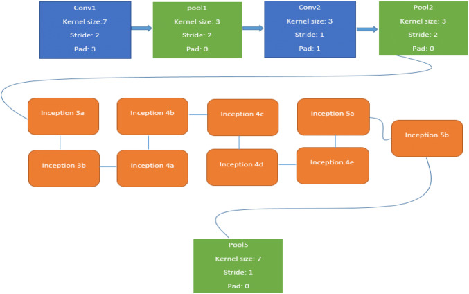
In the form of inception module has introduced a new level of organization. Simultaneously, they have increased the depth of the network. The computational cost of a deeper network is compensated by the optimization in the network. The small increase of computational requirements allows for a significant quality gain. Particular implementation of the inception architecture in the form of GoogleNet has won the ILSVRC 2014 image recognition competition (Szegedy et al. 2015). In this implementation, principle of NIN has been applied. In which additional 1 × 1 convolutional layers are followed by the rectified linear activation. Overall, GoogleNet consist of two convolutional, three pooling layers and nine Inception layers, where every inception layer contains six convolutional and one pooling layer (Fig. 2).

Fig. 2.

A simplified architecture of the CNN used in GoogleNet

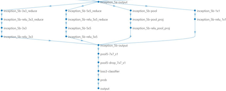
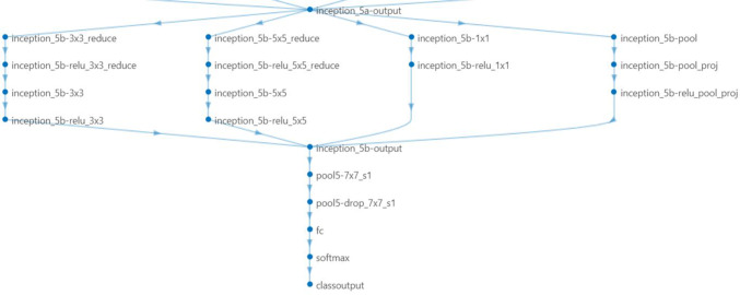
To classify new images (on prostate cancer data), we replaced last three layers with new layers to adapt new data set because the convolutional layers of the network extract image features that the last learnable layer and the final classification layer used to classify the input image. Pretrained network are configured for 1000 classes and these last three layers must be fine-tuned for the new classification problem. These two layers, ‘loss 3-classifier’ and ‘output’ in GoogLeNet, contain information on how to combine the features that the network extracts into class probabilities, a loss value, and predicted labels and we also replaced fully connected layer with a new fully connected layer where the number of outputs equal to the number of classes in the new data set (two in our case). We replaced these layers as shown in below Figs. 3 and 4.

Fig. 3.

Last layers of the GoogleNet before finetuning

Fig. 4.

Last layers of the GoogleNet after finetuning

Performance measures based on confusion matrix parameters

The performance using ML classifiers to detect the prostate cancer was measured on test data based on confusion matrix by computing sensitivity, specificity, PPV, NPV and Total Accuracy and confusion matrix is depicted in Fig. 5.

Fig. 5.

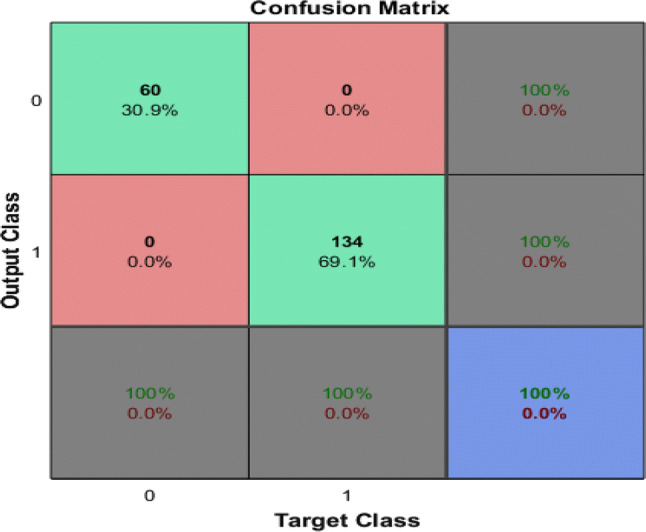
Confusion matrix for GoogleNet

Sensitivity

The sensitivity measure is used to check the ratio of subjects who test positive for the disease between those who have the disease. Mathematically, it is expressed as:

$$Sensitivity=\frac{\mathit{TP}}{TP+FN}$$ 5

i.e. the likelihood of positive test specified that patient has disease.

Specificity

Specificity measures the ratio of negatives that are properly identified. Mathematically, it is expressed as:

$$Specificity=\frac{\mathit{TN}}{TN+FP}$$ 6

i.e. likelihood of a negative test specified that patient is well.

Positive predictive value (PPV)

PPV is mathematically is expressed as:

$$PPV=\frac{\mathit{TP}}{TP+FP}$$ 7

where TP represent that the test makes a positive estimate and subject has a positive outcome under gold standard while FP is the event that test make a positive forecast and subject make a negative outcome.

Negative predictive value (NPV)

$$NPV=\frac{\mathit{TN}}{TN+FN}$$ 8

Total accuracy (TA)

The total accuracy is computed as:

$$TA=\frac{TP+TN}{TP+FP+FN+TN}$$ 9

Receiver operating curve (ROC)

The ROC is plotted against the true positive rate (TPR) i.e. sensitivity and false positive rate (FPR) i.e. specificity values of prostate and brachytherapy subjects. The average features values for brachytherapy subjects are classified as 1 and for prostate subjects are classified as 0. Then vector was passed to ROC function, which plots each example values against specificity and sensitivity values. To diagnose and visualize the performance of a model, ROC is one of the standard way to measure the performance (Hajian-Tilaki 2013). The TPR is plotted against y-axis and FPR is plotted against x-axis. The area under the curve (AUC) illustrate the part of a square unit. Its value falls among 0 and 1. AUC > 0.50 displays the separation. The higher AUC represents the better diagnostic system. Accurate positive cases divided by the sum of positive cases are denoted by TPR, whereas negative cases predicted as positive divided by the sum of negative cases are denoted by FPR.

Results and discussion

Performance of classification using deep learning pre-trained network (GoogleNet) was evaluated using different performance measures. In below Fig. 5, the first two diagonal cells show the number and percentage of correct classifications such as 60 cases of Brachytherapy are correctly classified. Brachytherapy samples are 30.9% of all training samples. Similarly, 134 cases are correctly classified as prostate. This corresponds to 69.1% of all samples. None of the sample is misclassified in both cases.

Out of 60 Brachytherapy predictions, 100% are correct. Similarly, out of 134 predictions, 100% are correct. Overall, 100% of the predictions are correct.

In this study, we have compared the results of machine learning classifiers (such as Bayes, decision tree, SVM Gaussian, SVM RBF, SVM polynomial by extracting and employing combination of features texture + morphological, EFDs + morphological outer performed as obtained by Hussain et al. (2018a, b) with the deep learning method (GoogleNet) using CNN approach. The highest performance using combination of features i.e. texture + morphological and EFDs + morphological were obtained using SVM Gaussian with as Sensitivity and TA (99.71%), specificity (99.58%), PPV (99.71%), NPV (99.58%), and AUC (1.00) followed by SVM Gaussian with texture + SIFT features i.e. sensitivity (98.83%), specificity (97.99%), PPV (98.83%), NPV (98.83%), and AUC (0.999). The GoogleNet using deep learning outer performed with Sensitivity, specificity, PPV, and TA of 100%, AUC of 1.00 as reflected in the below Fig. 6.

Fig. 6.

Performance evaluation comparison of ML methods with Deep Learning GoogleNet

At initial iterations and epoch 1, the mini-batch and validation accuracy was lower and increased with the increase in iterations and epoch 2. The accuracy of few selected iterations is reflected in the Fig. 7. At first iteration the mini-batch accuracy of 50%, at 12 iteration it was 90%, while a 100% at all other iterations. Similarly, validation accuracy at iteration 1 was 82.99%, 6 (98.97%), 12 (96.93%), 30 (100%), 40 (99.48%) and 45, 48, 84, 90 (100%).

Fig. 7.

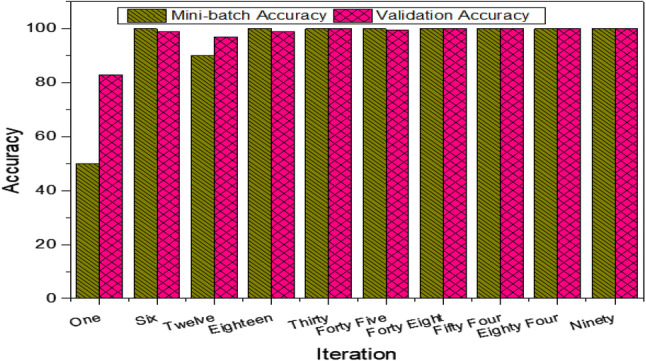
Performance measure using GoogleNet at different selected iterations

This Fig. 8 reflect the mini-batch and validation loss obtained using GoogleNet for selected iterations. As reflected in the Figure that first epoch and iterations up to 18, there was higher loss as lower accuracy was obtained, while second epoch and higher iterations the loss is minimized by increasing the performance accuracy. The mini-batch loss at iteration 1 was 0.7086, 6 (0.0210), 12 (0.1293), 18 (0.0504), 30 (0.0003), 45 (0.0002), 48 (0.0004), 54 and 90(0.000). Similarly, the validation loss obtained at each iteration was 1(0.4206), 6 (0.1025), 12 (0.1130), 18 (0.0357), 30 (0.0069), 45 (0.0091), 48 (0.0095), 54 (0.0079), 84 (0.0025) and 90 (0.0030).

Fig. 8.

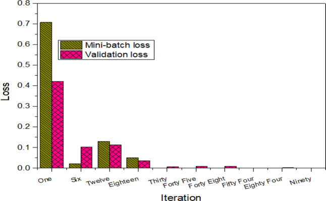
Loss at selected iterations using GoogleNet

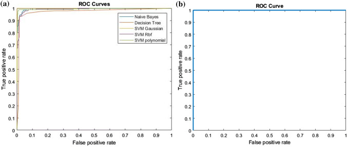
The ROC curves are drawn between true positive and false positive rate of prediction of training dataset. The combination of features such as texture + morphological gives highest AUC of 1.00 using SVM Gaussian followed by Bayes with AUC of 0.9469, SVM Polynomial with AUC of 0.9934, SVM RBF with AUC of 0.9911 and Decision Tree with AUC of 0.9731 as reflected in Fig. 9a and b. The GoogleNet using transfer learning approach of CNN gives AUC of 1.00 as reflected in Fig. 10.

Fig. 9.

a ROC using ML methods with texture + morphological features and b ROC using GoogleNet Deep Learning method

Fig. 10.

Training progress of GoogleNet

Training progress of GoogleNet are shown above, network is trained in two epochs approximately in each iteration increase in validation accuracy are observed. Validation are done after each 3^rd iteration, at first iteration validation accuracy is 61% after that accuracy is increased higher and in most of cases, the validation accuracy was obtained as 100%.

Conclusion

In the present study, a Deep learning convolution neural network (CNN) model was employed and performance was compared with machine learning techniques to detect the Prostate Cancer using Matlab version 2017b. A transfer learning approach was used to train the cancer images using GoogleNet from CNN. Multimodal features such as texture, morphological, entropy, SIFT and EFDs are extracted from cancer imaging database and performance was evaluated in terms of single and combination of features using robust machine learning techniques. The highest performance using machine learning techniques was obtained using SVM Gaussian with combination of features i.e. texture + morphological and EFDs + morphological with sensitivity & total accuracy of 99.71% was obtained followed by SVM Gaussian with texture + SIFT features with sensitivity of 98.83% and AUC of 0.999. The GoogleNet using Deep learning CNN approach outer performed by obtaining specificity, sensitivity, PPV and TA of 100% and AUC of 1.00.

Compliance with ethical standards

Conflict of interest

The Authors declares no conflict of interest.

References

- Akin O, Sala E, Moskowitz CS, Kuroiwa K, Ishill NM, Pucar D, Scardino PT, Hricak H. Transition zone prostate cancers: features, detection, localization, and staging at endorectal MR imaging. Radiology. 2006;239:784–792. doi: 10.1148/radiol.2392050949. [DOI] [PubMed] [Google Scholar]
- Asvadi NH, Afshari Mirak S, Mohammadian Bajgiran A, Khoshnoodi P, Wibulpolprasert P, Margolis D, Sisk A, Reiter RE, Raman SS. 3T multiparametric MR imaging, PIRADSv2-based detection of index prostate cancer lesions in the transition zone and the peripheral zone using whole mount histopathology as reference standard. Abdom Radiol. 2018;43:3117–3124. doi: 10.1007/s00261-018-1598-9. [DOI] [PMC free article] [PubMed] [Google Scholar]
- Bengio Y (2013) Deep learning of representations: looking forward. In: Lecture notes in computer science (including its subseries lecture notes in artificial intelligence and lecture notes in bioinformatics), 7978 LNAI, pp 1–37
- Bengio Y, Courville AC, Vincent P (2012) Unsupervised feature learning and deep learning: A review and new perspectives. CoRR. arxiv:1206.5538
- Bonzon P. Towards neuro-inspired symbolic models of cognition: linking neural dynamics to behaviors through asynchronous communications. Cogn Neurodyn. 2017;11:327–353. doi: 10.1007/s11571-017-9435-3. [DOI] [PMC free article] [PubMed] [Google Scholar]
- Cameron A, Modhafar A, Khalvati F, Lui D, Shafiee MJ, Wong A, Haider M (2014) Multiparametric MRI prostate cancer analysis via a hybrid morphological-textural model. In: Conference proceedings: annual international conference of the IEEE engineering in medicine and biology society. IEEE engineering in medicine and biology society. Conference 2014, pp 3357–3360 [DOI] [PubMed]
- Chen W, Zheng R, Baade PD, Zhang S, Zeng H, Bray F, Jemal A, Yu XQ, He J. Cancer statistics in China. CA Cancer J Clin. 2016;66:115–132. doi: 10.3322/caac.21338. [DOI] [PubMed] [Google Scholar]
- Chesnais AL, Niaf E, Bratan F, Mège-Lechevallier F, Roche S, Rabilloud M, Colombel M, Rouvière O. Differentiation of transitional zone prostate cancer from benign hyperplasia nodules: evaluation of discriminant criteria at multiparametric MRI. Clin Radiol. 2013;68:e323–e330. doi: 10.1016/j.crad.2013.01.018. [DOI] [PubMed] [Google Scholar]
- Chou R, Croswell JM, Dana T, Bougatsos C, Blazina I, Fu R. Review annals of internal medicine screening for prostate cancer: a review of the evidence for the U.S. preventive services task force. Ann Intern Med. 2011;155:375–386. doi: 10.7326/0003-4819-155-11-201112060-00375. [DOI] [PubMed] [Google Scholar]
- Costa DN, Pedrosa I, Donato F, Roehrborn CG, Rofsky NM. MR imaging-transrectal US fusion for targeted prostate biopsies: implications for diagnosis and clinical management. RadioGraphics. 2015;35:696–708. doi: 10.1148/rg.2015140058. [DOI] [PubMed] [Google Scholar]
- Doyle S, Madabhushi A, Feldman M, Tomaszeweski J (2006) A boosting cascade for automated detection of prostate cancer from digitized histology. In: Medical image computing and computer-assisted intervention—MICCAI 2006, Pt 2 4191, pp 504–511 [DOI] [PubMed]
- Eggener SE, Badani K, Barocas DA, et al. Gleason 6 prostate cancer: translating biology into population health. J Urol. 2015;194:626–634. doi: 10.1016/j.juro.2015.01.126. [DOI] [PMC free article] [PubMed] [Google Scholar]
- Eigen D, Puhrsch C, Fergus R (2014) Depth map prediction from a single image using a multi-scale deep network. In: NIPS, pp 1–9
- Fan Y, Shen D, Gur RC, Gur RE, Davatzikos C. COMPARE: classification of morphological patterns using adaptive regional elements. IEEE Trans Med Imaging. 2007;26:93–105. doi: 10.1109/TMI.2006.886812. [DOI] [PubMed] [Google Scholar]
- Girshick R, Donahue J, Darrell T, Berkeley UC, Malik J (2012) Girshick_Rich_Feature_Hierarchies_2014_CVPR_paper.pdf. 2–9
- Goodfellow I, Bengio Y, Courville A. Deep learning. Nature. 2016;521:800. [Google Scholar]
- Gutstein S, Fuentes O, Freudenthal E. Knowledge transfer in deep convolutional neural nets. Int J Artif Intell Tools. 2008;17:555–567. [Google Scholar]
- Hajian-Tilaki K. Receiver operating characteristic (ROC) curve analysis for medical diagnostic test evaluation. Casp J Intern Med. 2013;4:627–635. [PMC free article] [PubMed] [Google Scholar]
- Han SM, Lee HJ, Choi JY. Computer-aided prostate cancer detection using texture features and clinical features in ultrasound image. J Digit Imaging. 2008;21:121–133. doi: 10.1007/s10278-008-9106-3. [DOI] [PMC free article] [PubMed] [Google Scholar]
- He K, Zhang X, Ren S, Sun J (2016) Deep residual learning for image recognition, pp 770–778
- Hinton GE, Osindero S, Teh Y-W. Communicated by Yann Le Cun A Fast learning algorithm for deep belief nets 500 units 500 units. Neural Comput. 2006;18:1527–1554. doi: 10.1162/neco.2006.18.7.1527. [DOI] [PubMed] [Google Scholar]
- Hinton G, Deng L, Yu D, et al. Deep neural networks for acoustic modeling in speech recognition: the shared views of four research groups. IEEE Signal Process Mag. 2012;29:82–97. [Google Scholar]
- Homma T, Atlas L, Marks RJ., II An artificial neural network for spatio-temporal bipolar patters: application to phoneme classification. Adv Neural Inf Process Syst. 1988;1(1):31–40. [Google Scholar]
- Hricak H, Choyke PL, Eberhardt SC, Leibel S, Scardino PT. Imaging prostate cancer: a multidisciplinary perspective 1. Radiology. 2007;243:28–53. doi: 10.1148/radiol.2431030580. [DOI] [PubMed] [Google Scholar]
- Hussain L. Detecting epileptic seizure with different feature extracting strategies using robust machine learning classification techniques by applying advance parameter optimization approach. Cogn Neurodyn. 2018;12:271–294. doi: 10.1007/s11571-018-9477-1. [DOI] [PMC free article] [PubMed] [Google Scholar]
- Hussain L, Aziz W, Alowibdi JSJSJS, Habib N, Rafique M, Saeed S, Kazmi SZHSZ. Symbolic time series analysis of electroencephalographic (EEG) epileptic seizure and brain dynamics with eye-open and eye-closed subjects during resting states. J Physiol Anthropol. 2017;36:21. doi: 10.1186/s40101-017-0136-8. [DOI] [PMC free article] [PubMed] [Google Scholar]
- Hussain L, Ahmed A, Saeed S, Rathore S, Awan IA, Shah SA, Majid A, Idris A, Awan AA. Prostate cancer detection using machine learning techniques by employing combination of features extracting strategies. Cancer Biomark. 2018;21:393–413. doi: 10.3233/CBM-170643. [DOI] [PubMed] [Google Scholar]
- Hussain L, Saeed S, Awan IA, Idris A, Nadeem MSAA, Chaudhary Q-A, Chaudhry Q-A. Detecting brain tumor using machine learning techniques based on different features extracting strategies. Curr Med Imaging Former Curr Med Imaging Rev. 2018;14:595–606. doi: 10.2174/1573405614666180718123533. [DOI] [PubMed] [Google Scholar]
- Hussain L, Ali A, Rathore S, Saeed S, Idris A, Usman MU, Iftikhar MA, Suh DY. Applying bayesian network approach to determine the association between morphological features extracted from prostate cancer images. IEEE Access. 2018;7:1586–1601. [Google Scholar]
- Hussain L, Aziz W, Alshdadi AA, Ahmed Nadeem MS, Khan IR, Chaudhry Q-U-A. Analyzing the dynamics of lung cancer imaging data using refined fuzzy entropy methods by extracting different features. IEEE Access. 2019;7:64704–64721. [Google Scholar]
- Isselmou AEK, Zhang S, Xu G. A novel approach for brain tumor detection using MRI images. J Biomed Sci Eng. 2016;09:44–52. [Google Scholar]
- Karpathy A, Li FF (2015) Deep visual-semantic alignments for generating image descriptions. In: Proceedings of the IEEE computer society conference on computer vision and pattern recognition, pp 3128–3137 [DOI] [PubMed]
- Karpathy A, Toderici G, Shetty S, Leung T, Sukthankar R, Fei-Fei L (2014) Large-scale video classification with convolutional neural networks. In: IEEE conference on computer vision and pattern recognition (CVPR), 2014, pp 1725–1732
- Kattan MW, Potters L, Blasko JC, Beyer DC, Fearn P, Cavanagh W, Leibel S, Scardino PT. CME article brachytherapy in prostate cancer. Urology. 2001;4295:393–399. doi: 10.1016/s0090-4295(01)01233-x. [DOI] [PubMed] [Google Scholar]
- Khaki-Khatibi F, Nourazarian A, Ahmadi F, Farhoudi M, Savadi-Oskouei D, Pourostadi M, Asgharzadeh M. Relationship between the use of electronic devices and susceptibility to multiple sclerosis. Cogn Neurodyn. 2019;13:287–292. doi: 10.1007/s11571-019-09524-1. [DOI] [PMC free article] [PubMed] [Google Scholar]
- Krizhevsky A, Sutskever I, Hinton GE (2012) ImageNet classification with deep convolutional neural networks. Adv Neural Inf Process Syst 1097–1105
- LeCun Y, Bottou L, Bengio Y, Haffner P. Gradient-based learning applied to document recognition. Proc IEEE. 1998 doi: 10.1109/5.726791. [DOI] [Google Scholar]
- Lemaitre L, Puech P, Poncelet E, Bouyé S, Leroy X, Biserte J, Villers A. Dynamic contrast-enhanced MRI of anterior prostate cancer: morphometric assessment and correlation with radical prostatectomy findings. Eur Radiol. 2009;19:470–480. doi: 10.1007/s00330-008-1153-0. [DOI] [PubMed] [Google Scholar]
- Li J, Weng Z, Xu H, Zhang Z, Miao H, Chen W, Liu Z. Support Vector Machines (SVM) classification of prostate cancer Gleason score in central gland using multiparametric magnetic resonance images: a cross-validated study. Eur J Radiol. 2018;98:61–67. doi: 10.1016/j.ejrad.2017.11.001. [DOI] [PubMed] [Google Scholar]
- Lillicrap TP, Hunt JJ, Pritzel A, Heess N, Erez T, Tassa Y, Silver D, Wierstra D. Continuous control with deep reinforcement learning. Clin Linguist Phon. 2015 doi: 10.1561/2200000006. [DOI] [Google Scholar]
- Liu S, Liu S, Cai W, Pujol S, Kikinis R, Feng D (2014) Early diagnosis of Alzheimer’s disease with deep learning. In: 2014 IEEE 11th international symposium on biomedical imaging. IEEE, pp 1015–1018
- Liu Y, Yang G, Mirak SA, Hosseiny M, Azadikhah A, Zhong X, Reiter RE, Lee Y, Raman SS, Sung K. Automatic prostate zonal segmentation using fully convolutional network with feature pyramid attention. IEEE Access. 2019;7:163626–163632. [Google Scholar]
- Mooij G, Bagulho I, Huisman H (2018) Automatic segmentation of prostate zones
- Oto A, Kayhan A, Jiang Y, Tretiakova M, Yang C, Antic T, Dahi F, Shalhav AL, Karczmar G, Stadler WM. Prostate cancer: differentiation of central gland cancer from benign prostatic hyperplasia by using diffusion-weighted and dynamic contrast-enhanced MR imaging. Radiology. 2010;257:715–723. doi: 10.1148/radiol.10100021. [DOI] [PMC free article] [PubMed] [Google Scholar]
- Perez IM, Toivonen J, Movahedi P, Kiviniemi A, Pahikkala T, Aronen HJ, Jambor I (2016) Diffusion weighted imaging of prostate cancer: prediction of cancer using texture features from the parametric maps of the monoexponential and kurtosis functions using a grid approach. 0–7
- Pinto A, Alves V, Silva CA. Brain tumor segmentation using convolutional neural networks in MRI images. IEEE Trans Med Imaging. 2016;35:1240–1251. doi: 10.1109/TMI.2016.2538465. [DOI] [PubMed] [Google Scholar]
- Prostate MR (2018) Image database. http://prostatemrimagedatabase.com/index.html. Accessed 11 Mar 2018
- Rathore S, Hussain M, Khan A. Automated colon cancer detection using hybrid of novel geometric features and some traditional features. Comput Biol Med. 2015;65:279–296. doi: 10.1016/j.compbiomed.2015.03.004. [DOI] [PubMed] [Google Scholar]
- Ronneberger O, Fischer P, Brox T (2015) U-net: convolutional networks for biomedical image segmentation. In: Lecture notes in computer science (including its subseries lecture notes in artificial intelligence and lecture notes in bioinformatic). Springer, pp 234–241
- Schröder FH, Hugosson J, Roobol MJ, et al. Screening and prostate-cancer mortality in a randomized european study. N Engl J Med. 2009;360:1320–1328. doi: 10.1056/NEJMoa0810084. [DOI] [PubMed] [Google Scholar]
- Seltzer SE, Getty DJ, Tempany CM, Pickett RM, Schnall MD, McNeil BJ, Swets JA. Staging prostate cancer with MR imaging: a combined radiologist-computer system. Radiology. 1997;202:219–226. doi: 10.1148/radiology.202.1.8988214. [DOI] [PubMed] [Google Scholar]
- Shelhamer E, Long J, Darrell T. Fully convolutional networks for semantic segmentation. IEEE Trans Pattern Anal Mach Intell. 2017;39:640–651. doi: 10.1109/TPAMI.2016.2572683. [DOI] [PubMed] [Google Scholar]
- Siegel RL, Miller KD, Fedewa SA, Ahnen DJ, Meester RGS, Barzi A, Jemal A. Colorectal cancer statistics, 2017. CA Cancer J Clin. 2017;67:177–193. doi: 10.3322/caac.21395. [DOI] [PubMed] [Google Scholar]
- Szegedy C, Liu W, Jia Y, Sermanet P, Reed S, Anguelov D, Erhan D, Vanhoucke V, Rabinovich A (2015) Going deeper with convolutions, pp 1–9
- Taigman Y, Yang M, Ranzato M, Wolf L (2014) DeepFace: closing the gap to human-level performance in face verification. In: Proccedings of the computer society conference on computer vision and pattern recognition, pp 1701–1708
- Talcott JA, Manola J, Chen RC, Clark JA, Kaplan I, D’Amico AV, Zietman AL. Using patient-reported outcomes to assess and improve prostate cancer brachytherapy. BJU Int. 2014;114:511–516. doi: 10.1111/bju.12464. [DOI] [PubMed] [Google Scholar]
- Vos PC, Hambrock T, Barenstz JO, Huisman HJ. Computer-assisted analysis of peripheral zone prostate lesions using T2-weighted and dynamic contrast enhanced T1-weighted MRI. Phys Med Biol. 2010;55:1719–1734. doi: 10.1088/0031-9155/55/6/012. [DOI] [PubMed] [Google Scholar]
- Wall WA, Wiechert L, Comerford A, Rausch S. Towards a comprehensive computationalmodel for the respiratory system. Int J Numer Methods Biomed Eng. 2010;26:807–827. [Google Scholar]
- Yu KK, Hricak H. Imaging prostate cancer. J Urol. 2000;38:59–85. doi: 10.1016/s0033-8389(05)70150-0. [DOI] [PubMed] [Google Scholar]
- Zabihollahy F, Schieda N, Krishna Jeyaraj S, Ukwatta E. Automated segmentation of prostate zonal anatomy on T2-weighted (T2W) and apparent diffusion coefficient (ADC) map MR images using U-Nets. Med Phys. 2019;46:3078–3090. doi: 10.1002/mp.13550. [DOI] [PubMed] [Google Scholar]