

Abstract
Component-based software engineering is currently a development strategy used to improve complex embedded systems. The engineers have to deal with a large number of quality requirements (e.g. safety, security, availability, reliability, maintainability, portability, performance, and temporal correctness requirements), hence the development of complex embedded systems is becoming a challenging task. Enhancement of the quality prediction in component-based software engineering systems using soft computing techniques is the foremost intention of the research. Therefore, this paper proposes an extreme learning machine (ELM) classifier with the ant colony optimization algorithm and Nelder–Mead (ACO–NM) soft computing approach for component quality prediction. To promote efficient software systems and the ability of the software to work under several computer configurations maintainability, independence, and portability are taken as three core software components metrics for measuring the quality prediction. The ELM uses AC–NM for updating its weight to transform the quality constraints into objective functions for providing a global optimum quality prediction. The experimental results have shown that the proposed work gives an improved performance in terms of Sensitivity, Precision, Specificity, Accuracy, Mathews correlation coefficient, false positive rate, negative predictive value, false discovery rate, and rate of convergence.
Keywords: Ant colony optimization (ACO), Nelder–Mead (NM), Prediction quality, Soft computing, Extreme learning machine (ELM)
Introduction
Nowadays, an embedded system has been used in a very large number of applications in various fields such as satellite systems, manufacturing industries, automotive systems, medical applications, etc. (Guan and Offutt 2015). Thus the development of this system is becoming a challenging task that the system engineers need to deal with a large number of quality requirements such as reliability, availability, maintainability, security, safety, independence and portability (Garousi et al. 2018). The fulfillment of these quality requirements is important for project success and customer satisfaction. Hence, there was a growing need to predict and evaluate these quality measures in order to identify the problem earlier. In the early development process, traditional methods of Markov models, Queuing networks, Fault trees, Stochastic Petri Nets, and monolithic models are used to measures the quality properties (Cai et al. 2017). But, increasing scalability and complexity in systems, it is necessary to apply a component-based method in developing the complex embedded system (Chatzipetrou et al. 2019).
Currently, CBSE has become an emerging technology for predicting the quality of risk associated with component integration and selection, especially in complex embedded systems (Vale et al. 2016). CBSE builds new quality software using a method of software reuse (assembly, modification, application, and adaptation) from existing components such as software packages, web service, web-resource or any module (Kaindl et al. 2016). Using of software reuse method in CBSE increase the quality and productivity of the software in terms of reducing time, effort and costs (Shatnawi et al. 2017). Therefore, reusability plays a main role in building a high-quality software system (Padhy et al. 2018, 2019). Some of the following progressions performed by the CBSE are component search, selection, identification, recovery, and classification. The quality of the software is estimated by many factors such as software maintainability, portability, usability, testability, adaptability, reliability, etc. (Chatzipetrou et al. 2018; Patel and Kaur 2016). Among these, reliability quality factor tolerate faults and failures that occur during the software lifecycle (Preethi and Rajan 2016; Yamada and Tamura 2016). To uphold an efficient software system, maintainability should be considered as another essential quality aspect in the final stage of the software development lifecycle after completing the design, coding and testing phases (Kumar and Rath 2016; Almugrin et al. 2016). Working software with various computer configurations, portability is also considered the most essential quality aspect in the software system for measuring software quality (Haile and Altmann 2018). Apart from considering only reliability in software quality prediction, it is necessary to consider maintainability and portability as a series quality indexes based on software life cycles (Pennycook et al. 2019). Moreover, independence is also an important quality factor in the reusable module to define that the software does not depend on another module (Arar and Ayan 2017). In CBSE, various model is considered to enhance the applicability of the quality prediction, each of them differs in their quality prediction methods. Component-based software systems require a decision on the origin of the components to obtain the components. Factors such as influence on making decision and solution of choosing different components are presented (Wohlin et al. 2016). D Badampudi et al. (2016) identified that eleven factors are influencing to select a component origin with respect to outsourced components, open-source software, internal development components, and ready-to-use components.
To address the software quality problems, some of the recent techniques under software quality prediction (SQP) based on non-parametric techniques such as Machine Learning (ML), soft computing techniques and computational intelligence (CI) are presented (Malhotra 2015; Li et al. 2017). Some of the following ML techniques are Gradient boosting Decision tree; and soft computing techniques used for SQP are neural network (NN), fuzzy logic, genetic algorithm (GA), ant colony optimization (ACO), particle swarm optimization (PSO), feed forward neural network (FNN), recurrent neural network (RNN), artificial neural network (ANN), adaptive neuro-fuzzy inference system (ANFIS) and artificial bee colony (ACO) (Diwaker et al. 2018; Gavrilović et al. 2018; Ayon 2019). Various studies consider quality prediction based on software metric, ML, optimization schemes and hybrid combination (ML and optimization). The various software metric techniques like traditional software metrics, object-oriented software metrics, and process metrics are discussed first. Yadav and Yadav (2015) investigated that, to develop a reliability software product a quality prediction on the software development lifecycle is necessary. Hence, reliability relevant metrics were used as software metrics in their proposed fuzzy logic-based model. The purpose of this method is to measure the software metrics to check whether it is suitable for the fault indicator or for SQP. Thus reliability has been identified as a big software application issue when modifying coding styles and using various other parameters. To deal with this problem, Malhotra and Bansal (2015) proposed a new way based on an object-oriented metric for presenting a new predictive model, but software metrics are unable to produce satisfactory results when analyzing a complex software application. Therefore, a proper selection of software metrics will lead to a better prediction. The software requirement specification (SRS) is the fundamental expectation for customers to rebuild the software. Any errors or weaknesses injected at this stage create unexpected ripples in the software development cycle, resulting in poor quality in the software system. For this, Hejazi and Nasrabadi (2019) proposed a Granger Causality method as an autoregressive model together with the directed transfer function to evaluate the time series in the prediction model. Then Masood et al. (2018) used a method for selecting features in SRS to extract useful features which present information about the quality of SRS. First of all, the conversion of SRS into a graph is performed using different parameters of complexity, readability index, size and coupling. These extracted features form a bridge among the requirements and their impacts on quality. Then the following parameters are entered into a Fuzzy Inferencing System (FIS) to predict the quality of the final product.
Another problem that affects the quality performance in a software application is uncertainty. Where clustering, optimization, and classification techniques are performed to overcome uncertainty problems. Bashir et al. (2017) used a supervised classification method as a prediction model by using fault labels and historical software metrics. However, in some conditions, it is not enough to constructs accurate quality prediction models. Therefore, a powerful classifier is needed to accurately build a classification model or semi-supervised learning algorithms for training data. Zhang et al. (2017) used a nonnegative sparse graph-based label propagation method in semi-supervised learning for SQP to predict the labels of unlabeled software modules. When deep learning is applied as in regression problems, most of the high-level features are learned in the unsupervised learning stage (Liu et al. 2018).
Still, more effective optimization and more parameters need to be considered to achieve better quality estimation results (Ali et al. 2016). The neural network, soft computing, and hybrid methods provide a contribution to the proposed system as follows (Sheoran et al. 2016). Manjula and Florence (2019) consider the early software defects prediction as a challenging task when using software metrics, thus proposed a hybrid approach by combining GA with deep neural network (DNN–GA) for the feature optimization and classification. Wei et al. (2019) used a local tangent space alignment support vector machine (LTSA–SVM) algorithm for the software prediction model to extract the low-dimensional data structure and to reduce the data loss caused by the poor attributes under data non-linearity. Xu et al. (2019) proposed a new quality prediction technique by combining two Kernel principal component analysis (KPCA) and weighted extreme learning machine (WELM) techniques called KPWE. The two steps performed by a new framework are (1) Extracting correct data features and (2) Alleviating class imbalance. Dubey and Jasra (2017) presented a reliability assessment model based on an ANFIS for CBSE. The model aims to achieve a lower error than Milovancevic et al. (2018) used ANFIS for processing the vibration data to rank the input based on the impact on the vibration signal. Petkovic (2017) used ANFIS to estimate the friction factor. To further improve the precipitation concentration index (PCI), proper selection of parameters is important for PCI prediction to provide a selection procedure (Petković et al. 2017a; Nikolić et al. 2017). For that, Petkovic et al. (2014a, 2016) used ANFIS as a variable selection prediction model to find the most influential factors that affect the speed. To regulate the system of the speed. In Petković et al. (2013, 2014b) ANFIS is used as a regulator to operate at the high-efficiency point and to produce optimal coefficient value. Tomar et al. (2018) said artificial neural networks (ANN) learn from its failure and trains itself to avoid past mistakes. Measurement parameters such as goodness of fit, prediction ability for short-term prediction and long-term prediction prove to be better than traditional methods (Petković et al. 2017b). Therefore, a new efficient optimization algorithm of teaching–learning based optimization (TLBO) is used in ANN (ANN–TLBO). The ANN–TLBO introduces ANN on the basis of TLBO by transforming the constraints into an objective function to minimize the network error and to optimize the reliability and other cost function.
However, all of the above techniques used for SQP suffer various problems of accuracy, complexity and computational time. Thus, to overcome these problems, we have collected ideas from previous techniques to use more advanced optimization algorithms and neural networks to improve quality estimation. In our proposed system, numerous parameters are considered to improve our quality prediction to improve its sturdiness. Therefore, the proposed system uses a hybrid approach called, Extreme Learning Machine (ELM) based on the optimization of ant colony–Nelder–Mead (ACO–NM) ants with quality aspects of maintainability, independence and portability for a better quality prediction. Advanced neural network (ELM) and soft computing techniques (ACO–NM) provide better results than existing works.
The remaining sections of the manuscript are as follows:—Sect. 2 present the model description of proposed SQP. In Sect. 3, experimental result and analysis of the proposed method using ELM based ACO–NM method and its corresponding dataset descriptions are explained. Finally, the conclusion of the work are given in Sect. 4.
System model of software quality prediction
We introduce the ELM neural network with the ACO–NM algorithm for SQP to transform the following software constraints into objective functions. The proposed ELM model is designed on the basis of the single-layer feed forward network (SLFN). Therefore, a non-linear differentiable transfer function is used in the ELM approach for the activation function (Huang et al. 2015). Then, we have introduced a new efficient optimization method called ACO–NM to optimize the software quality metrics components like portability, independency, and maintainability. This optimization algorithm minimizes the network error by adjusting the weight value of the NN. The following Fig. 1 shows the proposed software component metrics quality prediction by using ELM with the ACO–NM method.
Fig. 1.

Proposed ELM classification and ACO–NM using software components metrics
In this proposed work, four input variables of interface surface consistency (ISC), bounded interface complexity metric (BICM), self-completeness components return value (SCCR) and self completeness components parameter (SCCP) are taken in the ELM classifier for both training and testing process. Then the hybrid ACO–NM algorithm is used for updating the optimal weight value. Finally, three expected output variables are taken in to account for better quality prediction measures are maintainability, independence, and portability. After that, the performance of the proposed work is analyzed in terms of sensitivity, precision, specificity, NPV, FPR, FDR, Accuracy, MCC and ROC.
Extreme learning machine (ELM)
ELM is a kind of advanced neural network, consists of three layers such as input layer, hidden layer (number of neurons) and an output layer. The input layer captures the input variable, hidden layers make a linear relationship among the variables and the output layer presents the predicted value. The following principle that differentiates ELM from other traditional NN is based on the parameters of the feed-forward network, inputs weights and biases provided to the hidden layer. In ELM, the bias of the hidden layer and input weight are randomly generated and the output is calculated by the Moore–Penrose generalized inverse of the hidden layer output matrix. The randomly chosen input weight and hidden layer biases learn the training samples with minimum error. After randomly choosing the input weights and the hidden layer biases, SLFNs can be simply considered as a linear system. The main advantage of ELM is, its structure does not depend on network parameters which produce stability. Hence it is useful for classification, regression, and clustering (Huang et al. 2015; Deo et al. 2016). Therefore, we adopted ELM as a classification model in predicting the software quality. Figure 2 shows the architecture of ELM with four input layers, ten hidden layers, and three output layers. The process of training and testing the ELM contains a network with two vectors of input vector and target output vector.
Fig. 2.

The architecture of the extreme learning machine
The ELM prediction model used for classification form a function , considering attributes as input vector and as output classification label target vector. In this proposed work, the attributes ISC, BICM, SCCR, and SCCP are considered as input metrics to predict software quality in terms of Maintainability, Independency and Portability. The classification labels vector denotes this software quality factors. Each of the input vector attributes describes the software components in the JavaBean software system. The objective consider is, to design an optimal input weight in SLFN with minimum error rate. Therefore, the evaluation of function is performed on the given dataset (), where is grouped into two parts of the training set and testing set . The learning process uses a back propagation algorithm for SLFN. Finally, the output classification label is evaluated on .
Consider training samples be , where indicates the input vector of jth samples with -dimensional attributes and indicates the jth output (target) vector with -dimension. In ELM, the bias to the hidden layer and input weights are generated randomly instead of tuning the network parameter. Therefore, the nonlinear system are transformed into linear system. The output function of SLFN are defined in mathematically as follows,
| 1 |
where denotes the jth sample output value, denotes the output weight vector connection between the jth hidden neurons to the output neurons, denotes the randomly assigned bias vector to the hidden neurons and the output neurons, and denotes the random input weight vector assigned between the input neurons and hidden neurons. The whole representation of indicates the output of jth hidden neurons with input samples.Training of the NN is performed, when the number of hidden neurons is equal to the distinct data (training) samples N = Q. The linear output representation of SLFN with hidden nodes and activation function of zero mean error in L samples is written as,
| 2 |
Then there should exist , and to satisfy this function
| 3 |
The matrix form for Eq. (3) is represented by
| 4 |
where represent the output matrix of the hidden layer
| 5 |
| 6 |
where Z indicates the training data target matrix. The activation function are the sigmoid in the hidden layer and a linear function for the output layer.The output weight value of the ELM network is derived by inverting the hidden layer matrix by using a Moore–Penrose generalized inverse function , which is given by
| 7 |
where denotes the Moore–Penrose generalized inverse of the hidden matrix (H), is the transposed matrix of and estimated output values from data sampling modelling used in process.Finally, the predicted values can be obtained by testing input vector with training dataset.
| 8 |
ELM present fast prediction performance as the output weights are computed randomly by the generated input weights and hidden biases using Moore–Penrose generalized inverse. But still there exist some non-optimal problems in and , cause overfitting in all training samples. Hence an enhancement must be made with prediction accuracy. Therefore, a hybrid ACO–NM optimization algorithm is used in ELM to train the NN in order to correct the network error and to optimize the weighting matrix of the NN, where the weights of each network are adjusted thus the network error is minimized.
Hybrid ACO–NM algorithm
Ant Colony Optimization is a type of meta-heuristic optimization algorithm inspired by the behavior of the real ants in which optimization problem are considered in terms of combinatorial. Whereas Nelder–Mead is a simplex direct search method used to solve unconstrained local nonlinear optimization problems. In ACO, ants deposit pheromones based on the response of other ants to minimize objective function, but in NM a simplex moves from an unconstrained search space to minimize objective function. Therefore, the ELM follows the ACO–NM algorithm for the weight optimization space in SLFN. The hybrid combination of ACO with NM is used to perform global optimization considering non-functional quality attributes such as maintainability, independence and portability. In hybrid ACO–NM algorithm, ACO performs exploration and NM algorithm performs exploration to quickly achieve global optimum, once the ACO algorithm finds a promising region. The two issues to be notified and corrected in performing hybrid optimal optimization in ELM are as follows,
Conversion of ACO algorithm to NM
Constructing initial simplex value to NM algorithm.
Conversion of ACO algorithm to NM
A proper standard deviation () must be chosen in conversion of ACO to NM that make a solution on decision making. Because, when the ACO algorithm starts to meet a global optimum, the decision making lies in the vicinity of the global optimum. This vicinity are used by NM to reach the global optimum quickly. In each of the iteration, need to be calculated. The conversion of ACO to NM is based on and specified value (). Choosing of large value for makes the conversion process earlier. If , ACO is allowed to run and if , ACO is shifted to NM. This might decrease the number of evaluation process.
Constructing initial simplex value to NM algorithm
It is essential to construct an initial simplex value in the NM method to point out the objective function values. The objective function must be evaluated for each initial population to obtain the best solution from the design variable. If the best solution is better than previous one, it is stored as the best solution. Therefore, before including the NM algorithm with ACO, we sort the solution in store based on its fitness value and divide them into a number of decision vector and select the first solution from to form an initial simplex value. This shows the variation present in the fitness value during the initial simplex. After creating simplex, the NM will run until finding the specified termination measures.
Hybrid ACO–NM algorithm in ELM
In this paper, we propose ACO–NM algorithm to train the SLFN, where the forward pass of back propagation algorithm is used for weight updating. The set of weights associated in NN form the decision vectors from input layers to hidden layers and hidden layers to output layers. Here we consider optimal input weight of SLFN as an objective function. A set of initially generated random variable are sent to the ACO algorithm to create a new solution sets until meeting the specified criteria. Here we yield termination measures as standard deviation (SD) or a certain number of iteration if the target value of SD is yet met. If the network error is more than the target value from the outcome ACO, a NM is used as simple method. The flowchart of ACO–NM algorithm is shown in Fig. 3.
Fig. 3.

Flow chart of proposed software quality prediction method in ELM–ACO–NM
Objective function
Objective function is evaluated for each initial population. Then the best solution is obtained by evaluating the mean value of the design variable. If the best solution is better than the previous one, then it is stored as the best solution.
The design of the optimal input weight on SLFNs using optimization model can be formulated by,
| 9 |
| 10 |
where denotes the real positive regularization parameter and denotes the target error.The optimal input weight matrix was derived as follows,
| 11 |
where denotes the identity matrix.
Similarly, to minimize the error between the desired output function and the actual output function . The optimal output weight on SLFNs using optimization model can be formulated by,
| 12 |
| 13 |
where denotes the real positive regularization parameter.
The optimal input weight matrix was derived as follows,
| 14 |
Component metrics for quality prediction in ELM
The several metrics for measuring reusability of software components, which include:—ISC, BICM, SCCR and SCCP. Following component metrics are given as the input to the ELM:
-
(i)
ISC (Interface Surface Consistency)
ISC is used to examine the consistency of the components interface parameter sorts, which depend on the consistency of the property compilation, components strategies and property complexity. The ISC expression is given as;
| 15 |
where SDM (i)—Standard deviation for the complexity of the ith strategy. SDP—Standard deviation for the property problem.
The above metrics carries the overall data about a components interface consistency. If the ISC value is high, it indicates the surface of the rough interface and some components may be difficult to maintain and integrate.
-
(ii)
BICM
BICM is used to evaluate the complexity of a software component, is given by the equation,
| 16 |
where SDM denotes the complexity of ith interference, SDP is the complexity of jth property, M and N, expresses to the count of component methods and properties separately, while and B are the weight values.
-
(iii)
SCCR
Inside a part c, SCCR(c) is said to be a rate of strategies with no arrival esteem in all techniques executed, which is given as;
| 17 |
where Bv(c)—Number of strategies without return value in c, B(c)—Quantity of techniques in c.
-
(iv)
SCCP
Inside a component c, SCCP (c) is said to be the rate of techniques with no parameters in all strategies actualized:
| 18 |
where Bp(c)—number of methods without parameters in c.
The following component (maintainability, independence and portability measures) metrics are taken as output from the ELM model.
-
(i)
Maintainability (M)Maintainability (M)
In an operational program there needed to alter and modify the fault. The maintainability is predicted with the below equation:
| 19 |
-
(ii)
Independence
The possibility of independence extends to overseeing collections in excess of two occasions or unpredictable elements, in which case the events are pairwise self-governing if each match is free of each other, and the events are ordinarily self-sufficient if each event is self-ruling of each other mix of events. When two events A and B, are freed, the likelihood of both happening is:
| 20 |
-
(iii)
Portability (P)
The software codebase highlight to have the capacity to reuse the current code as opposed to making new code while moving software from a context to another is known as Portability.
| 21 |
.
Experimental results
The implementation of the proposed method together with the existing method is performed on the MATLAB platform. In this paper, the ELM are performed in dataset of Java bean software (Tomar et al. 2018). The first 4 input neurons provided by dataset are BICM, ISC, SCCP, and SCCR said as a computed interface complexity metrics collected from super store with 10 hidden neutrons and one bias; and 3 output neurons named as Maintainability, Portability and Independence. The value for each metrics are provided in Table 1 and its corresponding output in Table 2.
Table 1.
Input Data of Java bean software components
| S. no. | Component | BICM | SCCP | ISC | SCCR |
|---|---|---|---|---|---|
| 1 | Gmail | 0.58 | 0.5273 | 0.58769 | 0.5091 |
| 2 | Gdata | 0.57 | 0.4828 | 0.68442 | 0.5287 |
| 3 | Gcalender | 0.47 | 0.45 | 0.5788 | 0.5167 |
| 4 | Gcontacts | 0.47 | 0.4775 | 0.39845 | 0.0631 |
| 5 | Gdocumments | 0.54 | 0.5098 | 0.62953 | 0.549 |
| 6 | Gstorage | 0.46 | 0.5686 | 0.50522 | 0.6176 |
| 7 | Amazonrequest | 0.49 | 0.55 | 0.4427 | 0.56 |
| 8 | Sqs | 0.56 | 0.6269 | 0.36929 | 0.5522 |
| 9 | Table | 0.45 | 0.4878 | 0.30318 | 0.5854 |
| 10 | Blob | 0.51 | 0.5727 | 0.73334 | 0.6636 |
| 11 | Gspreadsheets | 0.59 | 0.4435 | 0.77473 | 0.5217 |
| 12 | Simpledb | 0.45 | 0.5439 | 0.29006 | 0.5965 |
| 13 | Soap | 0.39 | 0.4712 | 0.38082 | 0.4904 |
| 14 | Rss | 0.52 | 0.6125 | 0.79353 | 0.6125 |
| 15 | Paapi | 0.39 | 0.5 | 0.27386 | 0.4722 |
| 16 | Mime | 0.53 | 0.5484 | 0.22685 | 0.6452 |
| 17 | Syslog | 0.73 | 0.6667 | 1.35463 | 0.619 |
| 18 | Queue | 0.48 | 0.5 | 0.53955 | 0.6316 |
| 19 | Ftp | 0.4 | 0.5143 | 0.23112 | 0.6429 |
| 20 | Pop | 0.47 | 0.4225 | 0.20733 | 0.5211 |
| 21 | PVTable | 0.48 | 0.5992 | 0.51112 | 0.5182 |
| 22 | Xmpp | 0.61 | 0.6304 | 0.98112 | 0.6739 |
| 23 | Smtp | 0.35 | 0.5333 | 0.15233 | 0.6 |
| 24 | Webdav | 0.47 | 0.6237 | 0.55864 | 0.6344 |
| 25 | PVCalendar | 0.62 | 0.5837 | 0.98199 | 0.5598 |
| 26 | S3 | 0.48 | 0.5769 | 0.5004 | 0.6154 |
| 27 | Whois | 0.44 | 0.6071 | 0.17239 | 0.6071 |
| 28 | atePicker | 0.49 | 0.5484 | 0.16701 | 0.5419 |
| 29 | Webupload | 0.44 | 0.5634 | 0.46281 | 0.5915 |
| 30 | Sapclient | 0.39 | 0.4528 | 0.14618 | 0.5849 |
| 31 | PVCalculator | 0.38 | 0.5844 | 0.17544 | 0.6364 |
| 32 | Azurerequest | 0.47 | 0.5567 | 0.27386 | 0.5567 |
| 33 | Telnet | 0.46 | 0.7333 | 0.21275 | 0.75 |
| 34 | PVTree | 0.51 | 0.6354 | 0.3558 | 0.5313 |
| 35 | PVChoice | 0.4 | 0.5806 | 0.29792 | 0.5484 |
Table 2.
Optimized output data of Java bean software components
| S. no. | Component | Maintainability | Independence | Portability |
|---|---|---|---|---|
| 1 | Gmail | 1 | 0.56 | 0.68 |
| 2 | Gdata | 1 | 0.42 | 0.77 |
| 3 | Gcalender | 1 | 1 | 0.9 |
| 4 | Gcontacts | 0.97 | 1 | 0.73 |
| 5 | Gdocumments | 0.63 | 0.91 | 0.67 |
| 6 | Gstorage | 1 | 0.8 | 0.8 |
| 7 | Amazon request | 0.99 | 0.79 | 1 |
| 8 | Sqs | 0.95 | 1 | 1 |
| 9 | Table | 0.51 | 0.89 | 0.78 |
| 10 | Blob | 0.2 | 1 | 1 |
| 11 | Gspreadsheets | 0.2 | 0.85 | 1 |
| 12 | Simpledb | 1 | 1 | 0.78 |
| 13 | Soap | 1 | 0.65 | 0.7 |
| 14 | Rss | 1 | 0.74 | 0.54 |
| 15 | Paapi | 0.71 | 1 | 1 |
| 16 | Mime | 0.87 | 1 | 0.73 |
| 17 | Syslog | 0.78 | 0.97 | 1.52 |
| 18 | Queue | 0.73 | 0.5 | 0.81 |
| 19 | Ftp | 1 | 1 | 1 |
| 20 | Pop | 1 | 0.95 | 0.14 |
| 21 | PVTable | 0.89 | 0.89 | 0.91 |
| 22 | Xmpp | 0.76 | 1 | 1 |
| 23 | Smtp | 1 | 1 | 0.84 |
| 24 | Webdav | 0.72 | 0.87 | 1 |
| 25 | PVCalendar | 0.79 | 0.75 | 1 |
| 26 | S3 | 0.68 | 0.83 | 1 |
| 27 | Whois | 0.77 | 1 | 1 |
| 28 | atePicker | 1 | 1 | 0.75 |
| 29 | Webupload | 1 | 0.84 | 0.99 |
| 30 | Sapclient | 1 | 1 | 1 |
| 31 | PVCalculator | 0.53 | 0.47 | 0.88 |
| 32 | Azurerequest | 0.43 | 0.65 | 1 |
| 33 | Telnet | 1 | 0.47 | 0.8 |
| 34 | PVTree | 0.34 | 0.98 | 1 |
| 35 | PVChoice | 1 | 1 | 1 |
The following techniques are utilized for the performance analysis named as: Precision, sensitivity, specificity, FPR, NPV, accuracy, FDR, ROC (iterations before convergence) and MCC and compare the performance by these methods.
-
(i)
Precision
| 22 |
where TP, TN—True Positive and True Negative, FP, FN—False Positive and False Negative.
Precision is a measure of accuracy, which represents the relationship between the numbers of TP and FN. The predicted components are divided by the total number of positive elements. The performance analysis of the proposed method using Java beans datasets is shown in Fig. 4.
Fig. 4.
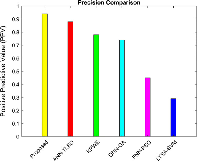
Performance analysis of precision using ELM ACO–Nelder method Java bean software components
In this analysis, the proposed method is compared with some existing prediction methods ANN-TLBO, FNN-PSO KPWE, LTSA-SVM and DNN-GA methods. Figure 4 illustrates the precision value of the proposed method using the Java bean dataset is 0.93 PPV higher than the existing methods.
-
(ii)
Sensitivity
| 23 |
The result of the sensitivity analysis on dataset for the proposed method and existing methods are presented in Fig. 5. Here, the low sensitivity indicates that there are many high-risk components in the software. Figure 5 shows the performance of the sensitivity comparison, here the proposed method achieve 1.01 value. The sensitivity of the proposed method is better than the existing methods ANN-TLBO, FNN-PSO KPWE, LTSA-SVM and DNN-GA.
Fig. 5.

Analysis of sensitivity using ELM ACO–Nelder method Java bean software components
-
(iiI)
Specificity
| 24 |
Clar Fig. 6 show the specificity performance in Java bean software component. Where greater specificity and sensitivity is to consider the best performance classifier. According to that, the specificity of the proposed approach in Java bean components showed a value of 0.92 higher than the existing methods.
Fig. 6.

Analysis of specificity using ELM ACO–Nelder method for Java bean software components
-
(iv)
NPV
| 25 |
In Fig. 7, the performance comparison of the NPV with respect to the proposed and existing method is shown. This NPV analysis is used to find the true negative value. The comparison value for the negative predictive value in Java bean shows 1.01 for the proposed method.
Fig. 7.

Analysis of NPV using ELM ACO–Nelder method for Java bean software components
-
(v)
FPR
| 26 |
Generally, the FPR is explained based on the function of fall-out. The ratio between the numbers of false predictions of negative events and the total number of true negative events is known as FPR. Figure 8 illustrate the FPR result for Java bean dataset. The trends of the proposed and existing methods ANN–TLBO, FNN–PSO KPWE, LTSA–SVM and DNN–GA are clearly visible in the results, the detection rate is influenced by the false positive rate and the proposed system using a Java bean dataset presents a comparable improvement in the detection rate.
Fig. 8.
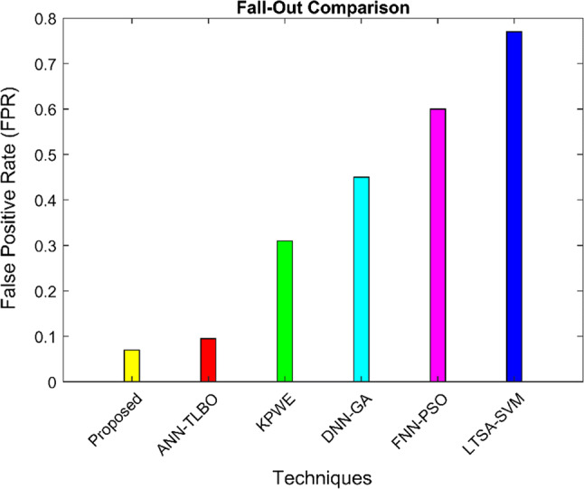
Performance analysis of FPR using ELM ACO–Nelder method Java bean software components
-
(vi)
False Discovery Rate (FDR)
| 27 |
Figure 9 shows the FDR performance in Java bean dataset. In a set of predictions, the measurement of false predictions is known as FDR. The proposed algorithm provides a lower value of 0.06 FDR in the Java bean produces the maximum prediction compared to the other existing algorithms.
Fig. 9.

Performance analysis of FDR using ELM ACO–Nelder method Java bean software components
-
(vii)
Accuracy
| 28 |
Figure 10 illustrate the accuracy performance of the proposed method using Java bean dataset. The accuracy of the Java bean dataset using proposed is 96.2% better than the existing prediction algorithm ANN–TLBO, FNN–PSO KPWE, LTSA–SVM and DNN–GA.
Fig. 10.

Performance analysis of accuracy using ELM ACO–Nelder method
-
(viii)
MCC
| 29 |
Figure 11 shows the performance of MCC using java bean dataset. The performance of proposed method obtains 0.92 for MCC and for the same execution the ANN TLBO algorithm has a value of 0.89, FNN–PSO has a value of 0.46, LTSA–SVM has 0.37 and 0.6 for DNN–GA.
Fig. 11.
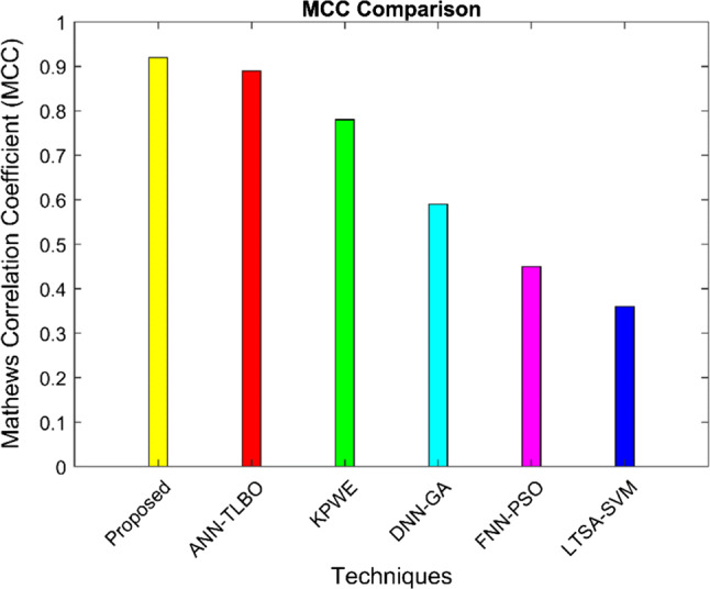
Performance analysis of Mathew’s correlation coefficient (MCC) using ELM ACO–Nelder method java bean software components
Table 3 represents the performance status of proposed method with the existing methods for both software component dataset.
Table 3.
Performance Status for Proposed Work and Compare it with the Existing Method using Java bean software component dataset
| Methods | Sensitivity | Accuracy | Specificity | Precision NPV |
FPR | FDR | MCC | |
|---|---|---|---|---|---|---|---|---|
| FNN–PSO (Ayon 2019) | 0.95 | 0.99 | 54.2 | 0.35 | 0.48 | 0.6 | 0.14 | 0.46 |
| DNN–GA (Manjula and Florence 2019) | 0.979 | 0.68 | 66.4 | 0.54 | 0.76 | 0.45 | 0.15 | 0.6 |
| LTSA–SVM (Wei et al. 2019) | 0.96 | 0.94 | 36.7 | 0.28 | 0.29 | 0.78 | 0.32 | 0.37 |
| KPWE (Xu et al. 2019) | 0.98 | 0.99 | 89 | 0.68 | 0.78 | 0.3 | 0.40 | 0.78 |
| ANN–TLBO (Tomar et al. 2018) | 1 | 1 | 94.44 | 0.90 | 0.88 | 0.099 | 0.11 | 0.89 |
| Proposed (ELM based ACO–NM) | 1.01 | 1.01 | 96.2 | 0.92 | 0.93 | 0.09 | 0.062 | 0.92 |
The convergence rate of the proposed and existing works is shown in Fig. 12. Compared to conventional approaches, the ELM ACO–NM shows the fastest convergence rate. This work has improved the execution of the quality prediction of a component-based software framework. Execution of specificity, sensitivity, precision, FPR, NPV, FDR, MCC and accuracy enhanced by the proposed ELM ACO–NM method. Our proposed work offers better performance by comparing performance with these techniques.
Fig. 12.

Performance of convergence rate using ELM ACO–NM method in Java bean software components
Conclusion
In this proposed strategy, an ELM-based ACO–NM method is introduced as a prediction model in measuring the quality component of the software in transforming quality constraints into objective functions. ELM is a type of neural system that uses SLFN as a basic model to train the network more quickly with individual weights. The global optimum quality prediction is the main objective of this paper. Then the ACO–NM algorithm is used in the ELM classifier. This algorithm is used to find the optimal solution based on the objective function. The experiment is evaluated in the MATLAB platform and the effectiveness of the proposed algorithm is conducted in one reference datasets of Java beans software components. Finally, the performance is analyzed in terms of precision, sensitivity, specificity, NPV, Accuracy, FDR, FPR, and MCC. Based on the experimental results, the proposed method offers better performance than the existing ANN–TLBO, FNN–PSO, DNN–GA, KPWE and LTSA–SVM methods.
Footnotes
Publisher's Note
Springer Nature remains neutral with regard to jurisdictional claims in published maps and institutional affiliations.
References
- Ali A, Choudhary K, Sharma A (2016) Software quality prediction using random particle swarm optimization (PSO). In: 2016 International conference on circuit, power and computing technologies (ICCPCT). IEEE, pp 1–6
- Almugrin S, Albattah W, Melton A. Using indirect coupling metrics to predict package maintainability and testability. J Syst Softw. 2016;121:298–310. [Google Scholar]
- Arar ÖF, Ayan K. A feature dependent Naive Bayes approach and its application to the software defect prediction problem. Appl Soft Comput. 2017;59:197–209. [Google Scholar]
- Ayon SI (2019) Neural network based software defect prediction using genetic algorithm and particle swarm optimization. In: 2019 1st international conference on advances in science, engineering and robotics technology (ICASERT). IEEE, pp 1–4
- Badampudi D, Wohlin C, Petersen K. Software component decision-making: In-house, OSS, COTS or outsourcing—a systematic literature review. J Syst Softw. 2016;121:105–124. [Google Scholar]
- Bashir K, Li T, Yohannese CW, Mahama Y (2017) Enhancing software defect prediction using supervised-learning based framework. In: 2017 12th international conference on intelligent systems and knowledge engineering (ISKE). IEEE, pp 1–6
- Cai BL, Zhang RQ, Zhou XB, Zhao LP, Li KQ. Experience availability: tail-latency oriented availability in software-defined cloud computing. J Comput er Sci Technol. 2017;32(2):250–257. [Google Scholar]
- Chatzipetrou P, Papatheocharous E, Wnuk K, Borg M, Alégroth E, Gorschek T. Component attributes and their importance in decisions and component selection. Softw Qual J. 2019 [Google Scholar]
- Chatzipetrou P, Alégroth E, Papatheocharous E, Borg M, Gorschek T, Wnuk K (2018). Component selection in software engineering-which attributes are the most important in the decision process? In: 2018 44th Euromicro conference on software engineering and advanced applications (SEAA). IEEE, pp 198–205
- Deo RC, Samui P, Kim D. Estimation of monthly evaporative loss using relevance vector machine, extreme learning machine and multivariate adaptive regression spline models. Stoch Env Res Risk Assess. 2016;30(6):1769–1784. [Google Scholar]
- Diwaker C, Tomar P, Poonia RC, Singh V. Prediction of software reliability using bio inspired soft computing techniques. J Med Syst. 2018;42(5):93. doi: 10.1007/s10916-018-0952-3. [DOI] [PubMed] [Google Scholar]
- Dubey SK, Jasra B. Reliability assessment of component based software systems using fuzzy and ANFIS techniques. Int J Syst Assur Eng Manag. 2017;8(2):1319–1326. [Google Scholar]
- Garousi V, Felderer M, Karapıçak ÇM, Yılmaz U. What we know about testing embedded software. IEEE Softw. 2018;35(4):62–69. [Google Scholar]
- Gavrilović S, Denić N, Petković D, Živić NV, Vujičić S. Statistical evaluation of mathematics lecture performances by soft computing approach. Comput Appl Eng Edu. 2018;26(4):902–905. [Google Scholar]
- Guan J, Offutt J (2015) A model-based testing technique for component-based real-time embedded systems. In: 2015 IEEE eighth international conference on software testing, verification and validation workshops (ICSTW). IEEE, pp 1–10
- Haile N, Altmann J. Evaluating investments in portability and interoperability between software service platforms. Future Gener Comput Syst. 2018;78:224–241. [Google Scholar]
- Hejazi M, Nasrabadi AM. Prediction of epilepsy seizure from multi-channel electroencephalogram by effective connectivity analysis using Granger causality and directed transfer function methods. Cogn Neurodyn. 2019;13(5):461–473. doi: 10.1007/s11571-019-09534-z. [DOI] [PMC free article] [PubMed] [Google Scholar]
- Huang G, Huang GB, Song S, You K. Trends in extreme learning machines: a review. Neural Networks. 2015;61:32–48. doi: 10.1016/j.neunet.2014.10.001. [DOI] [PubMed] [Google Scholar]
- Kaindl H, Popp R, Hoch R, Zeidler C (2016) Reuse vs. reusability of software supporting business processes. In: International conference on software reuse. Springer, Cham, pp 138–145
- Kumar L, Rath SK. Hybrid functional link artificial neural network approach for predicting maintainability of object-oriented software. J Syst Softw. 2016;121:170–190. [Google Scholar]
- Li J, He P, Zhu J, Lyu MR (2017) Software defect prediction via convolutional neural network. In: 2017 IEEE international conference on software quality, reliability and security (QRS). IEEE, pp 318–328
- Liu Y, Yang C, Gao Z, Yao Y. Ensemble deep kernel learning with application to quality prediction in industrial polymerization processes. Chemom Intell Lab Syst. 2018;174:15–21. [Google Scholar]
- Malhotra R. A systematic review of machine learning techniques for software fault prediction. Appl Soft Comput. 2015;27:504–518. [Google Scholar]
- Malhotra R, Bansal AJ. Fault prediction considering threshold effects of object-oriented metrics. Expert Syst. 2015;32(2):203–219. [Google Scholar]
- Manjula C, Florence L. Deep neural network based hybrid approach for software defect prediction using software metrics. Cluster Comput. 2019;22(4):9847–9863. [Google Scholar]
- Masood MH, Khan MJ (2018). Early software quality prediction based on software requirements specification using fuzzy inference system. In: International conference on intelligent computing. Springer, Cham, pp 722–733
- Milovančević M, Nikolić V, Petkovic D, Vracar L, Veg E, Tomic N, Jović S. Vibration analyzing in horizontal pumping aggregate by soft computing. Measurement. 2018;125:454–462. [Google Scholar]
- Nikolić V, Mitić VV, Kocić L, Petković D. Wind speed parameters sensitivity analysis based on fractals and neuro-fuzzy selection technique. Knowl Inf Syst. 2017;52(1):255–265. [Google Scholar]
- Padhy N, Singh RP, Satapathy SC. Software reusability metrics estimation: algorithms, models and optimization techniques. Comput Electr Eng. 2018;69:653–668. [Google Scholar]
- Padhy N, Singh RP, Satapathy SC. Enhanced evolutionary computing based artificial intelligence model for web-solutions software reusability estimation. Cluster Comput. 2019;22(4):9787–9804. [Google Scholar]
- Patel S, Kaur J (2016) A study of component based software system metrics. In: 2016 International conference on computing, communication and automation (ICCCA). IEEE, pp 824–828
- Pennycook SJ, Sewall JD, Lee VW. Implications of a metric for performance portability. Future Gener Comput Syst. 2019;92:947–958. [Google Scholar]
- Petković D. Prediction of laser welding quality by computational intelligence approaches. Optik. 2017;140:597–600. [Google Scholar]
- Petković D, Ab Hamid SH, Ćojbašić Ž, Pavlović NT. Adapting project management method and ANFIS strategy for variables selection and analyzing wind turbine wake effect. Nat Hazards. 2014;74(2):463–475. [Google Scholar]
- Petković D, Gocic M, Trajkovic S, Milovančević M, Šević D. Precipitation concentration index management by adaptive neuro-fuzzy methodology. Clim Change. 2017;141(4):655–669. [Google Scholar]
- Petković D, Nikolić V, Mitić VV, Kocić L. Estimation of fractal representation of wind speed fluctuation by artificial neural network with different training algorothms. Flow Meas Instrum. 2017;54:172–176. [Google Scholar]
- Petković D, Pavlović NT, Ćojbašić Ž. Wind farm efficiency by adaptive neuro-fuzzy strategy. Int J Electr Power Energy Syst. 2016;81:215–221. [Google Scholar]
- Petković D, Ćojbašić Ž, Nikolić V, Shamshirband S, Kiah MLM, Anuar NB, Wahab AWA. Adaptive neuro-fuzzy maximal power extraction of wind turbine with continuously variable transmission. Energy. 2014;64:868–874. [Google Scholar]
- Petković D, Ćojbašič Ž, Nikolić V. Adaptive neuro-fuzzy approach for wind turbine power coefficient estimation. Renew Sustain Energy Rev. 2013;28:191–195. [Google Scholar]
- Preethi W, Rajan MB (2016) Survey on different strategies for software reliability prediction. In: 2016 International conference on circuit, power and computing technologies (ICCPCT). IEEE, pp 1–3
- Shatnawi A, Seriai AD, Sahraoui H, Alshara Z. Reverse engineering reusable software components from object-oriented APIs. J Syst Softw. 2017;131:442–460. [Google Scholar]
- Sheoran K, Tomar P, Mishra R. Software quality prediction model with the aid of advanced neural network with HCS. Proc Comput Sci. 2016;92:418–424. [Google Scholar]
- Tomar P, Mishra R, Sheoran K. Prediction of quality using ANN based on Teaching-Learning Optimization in component-based software systems. Softw Practice Exp. 2018;48(4):896–910. [Google Scholar]
- Vale T, Crnkovic I, De Almeida ES, Neto PADMS, Cavalcanti YC, de Lemos Meira SR. Twenty-eight years of component-based software engineering. J Syst Softw. 2016;111:128–148. [Google Scholar]
- Wei H, Hu C, Chen S, Xue Y, Zhang Q. Establishing a software defect prediction model via effective dimension reduction. Inf Sci. 2019;477:399–409. [Google Scholar]
- Wohlin C, Wnuk K, Smite D, Franke U, Badampudi D, Cicchetti A (2016) Supporting strategic decision-making for selection of software assets. In International conference of software business. Springer, Cham, pp 1–15
- Xu Z, Liu J, Luo X, Yang Z, Zhang Y, Yuan P, Zhang T. Software defect prediction based on kernel PCA and weighted extreme learning machine. Inf Softw Technol. 2019;106:182–200. [Google Scholar]
- Yadav HB, Yadav DK. A fuzzy logic based approach for phase-wise software defects prediction using software metrics. Inf Softw Technol. 2015;63:44–57. [Google Scholar]
- Yamada S, Tamura Y (2016) Software reliability. In: OSS reliability measurement and assessment. Springer, Cham, pp 1–13
- Zhang ZW, Jing XY, Wang TJ. Label propagation based semi-supervised learning for software defect prediction. Autom Softw Eng. 2017;24(1):47–69. [Google Scholar]