Abstract
There is a need to develop more advanced tools to improve guidance on physical exercise to reduce risk of adverse events and improve benefits of exercise. Vast amounts of data are generated continuously by Personal Monitoring Devices (PMDs) from sports events, biomedical experiments, and fitness self-monitoring that may be used to guide physical exercise. Most of these data are sampled as time- or distance-series. However, the inherent high-dimensionality of exercise data is a challenge during processing. As a result, current data analysis from PMDs seldomly extends beyond aggregates.
Common challanges are:
-
•
alterations in data density comparing the time- and the distance domain;
-
•
large intra and interindividual variations in the relationship between numerical data and physiological properties;
-
•
alterations in temporal statistical properties of data derived from exercise of different exercise durations.
These challenges are currently unresolved leading to suboptimal analytic models. In this paper, we present algorithms and approaches to address these problems, allowing the analysis of complete PMD datasets, rather than having to rely on cumulative statistics. Our suggested approaches permit effective application of established Symbolic Aggregate Approximation modeling and newer deep learning models, such as LSTM.
Keywords: Symbolic aggregate approximation, SAX, Time series, Distance series, Sports events
Graphical abstract
Specifications table
| Subject Area: | Computer Science |
| More specific subject area: | Biomedical Data Analysis |
| Method name: | Symbolic Aggregate Approximation |
| Name and reference of original method: | J. Lin, E. Keogh, S. Lonardi, and B. Chiu, “A symbolic representation of time series, with implications for streaming algorithms,” in Proceedings of the 8th ACM SIGMOD workshop on Research issues in data mining and knowledge discovery - DMKD ’03, San Diego, California, 2003, p. 2, doi: 10.1145/882,082.882086. |
| Resource availability: |
Method details
Physical exercise is important for healthy living but represents a potential risk of sudden death in susceptible individuals. Advanced analysis of the relationship between different types of sensor data acquired during exercise may be valuable both in improving benefits and reducing risk of physical exercise [22]. Vast amounts of data are generated continuously by Personal Monitoring Devices (PMDs) in settings ranging from sport laboratory experiments, through supervised living (e.g. elderly homes), to everyday activities and fitness self-monitoring. Most of these data are of time-series or similar character, where data are recorded continuously, often with 1 s precision. Two of the most typical examples are continuous heart rate monitoring and power output monitoring during exercise such as running or cycling. Due to challenges related to the inherent high-dimensionality of time-series data, existing analytic approaches do not provide solutions that fully exploit the information generated from PMD data. As a result, analysis of data from PMDs is mostly limited to aggregates, e.g. average heart rate or maximum power output during exercise.
Current methods that may be used to analyze PMD data
There are many approaches that are used to model time series, these models have advantages and disadvantages that influence their relevance for the analysis of PMD data. Arguably, the most established approach for generic time series analysis is Autoregressive Integrated Moving Average (ARIMA) [1]. ARIMA models are usually applied following the so-called Box-Jenkins approach [2], which consist of: (1) model identification ensuring stationarity and removing seasonality; (2) parameter estimation using computational algorithms to fit model parameters; and finally (3) model checking. However, ARIMA is seldomly applied to long multivariate time series due to computational costs [20]. ARIMA modeling requires time series to be stationary and it is a property difficult to achieve in PMD data.
Partial Aggregate Averaging (PAA) and, in particular, Symbolic Aggregate Approximation (SAX) were developed to reduce dimensionality of time series data in a way that leads to a minimal loss of information [3]. These methods allow for improved pattern detection and search by enabling use of text mining algorithms in some implementations. They do not impose any additional statistical properties on the time series.
Since the initial publication in 2003 SAX has become a widely adopted method. By May 2019, a total of 1931 scientific works referenced the original SAX paper [10], 1060 referenced the updated SAX paper [3], and 254 scientific works referenced the extended iSAX paper [4]. Among these publications, around 180 papers had a primary focus on medicine, biomedicine or sport science. Banaee et al. used SAX for generating a textual overview of a patient from a large dataset, but did not compare between patients [17]. Oates et al. used SAX for time-series classification, but study participants were mostly motionless during measurements reducing common challenges of exercise data analysis such as large variable ranges, noise and alterations in the relationship between variables and the time/distance domain [18]. Authors noticed potential problems with representation of some values, but the problem was not discussed in depth. Milanko et al. predominantly focused on binary changes between exercise sets and rest periods, thereby not addressing problems related to graded interactions between variables [19].
The majority of works, however, use SAX for analysis of ECG, EEG, PPG, accelerometer/inertia sensor data or changes in HRV. These measures have a strictly defined value ranges that depend on the sensors or measurement methods used, rather than on variations between individual study subjects. Many papers referencing one of the SAX papers often refer to SAX as a possible tool without applying it to the presented problem. More challenging tasks, such as correct data scaling or analysis of complex data interactions between different types of PMD data, are sometimes acknowledged, but not addressed in depth.
Recently, a proliferation of deep learning approaches to time series analysis, particularly in the form of Long Short-Term Memory networks (LSTM), has emerged [21]. Since deep learning approaches have a much shorter history than SAX, fewer relevant publications were identified. Lipton et al. used LSTM for modeling of data from intensive care patients; however, they resampled all data to hourly means [5]. Pathinarupothi et al. used deep learning on instantaneous heart rate data to detect sleep apnea [6]. However, their implementation used Heart Rate Variability (HRV) and did not deal with the actual HR signal. Swapna et al. applied deep learning to heart rate signals for detection of diabetes [7]. However, also in this case only HRV was used, and time series aspect of HR was not addressed. Zhang et al. and many others also limited heart rate analysis only to HRV [8].
In contrast, Guan et al. applied LSTM to the actual heart rate data [9]. However, there are several limitations to their studies: participants were in a narrow range of maximum heart rate, data was only analyzed as a small manually labeled part of the full dataset and no distance information was present.
PAA and SAX have traditionally been used when the goal of time-series analysis is to model and compare. Deep learning approaches are usually used when the goal of the analysis is prediction. All these methods can be used for detection of anomalies either by comparison to a template, in case of SAX, or by deviation from the expected value in case of deep learning such as LSTM.
Methodological challenges related to current methods
There are several methodological challenges related to the use of SAX and deep learning in the analysis of PMD data in a real-life situation.
Problem 1: the first challenge is that SAX and deep learning assume that data is collected at a fixed rate, for example heart rate per second. However, when PMDs are used in a real-life situation, it is also of interest to analyze PMD data in relation to other variables such as distance moved or to power-output. If PMD data has been sampled at a fixed time-interval, data density will be uneven if data are analyzed in relation to distance or aggregated power-output (work performed). For example, a run in an undulating terrain will cause variations in running velocity that increase data density during up-hill runs and decreased data density during down-hill runs. In the present work, the problems related to variable data densities are referred to as Problem 1.
Problem 2: current methods assume that a given signal value represents the same physiological entity in all individuals. However, this is not necessarily true. For example, the heart rate response to exercise is age dependent and relates to training condition. This problem is annotated Problem 2.
Problem 3: typical preprocessing applied before SAX and deep learning can deal with certain amount of noise and outliers. However, the relationship between different types of PMD data in the beginning of an activity might exhibit very different characteristics compared during the course of strenuous exercise. We will refer to this challenge as Problem 3.
Methods validation
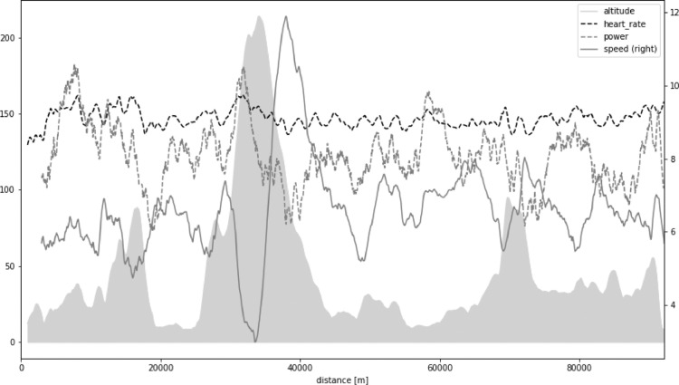
The present work is based upon PMD data derived from the North Sea Race Endurance Exercise Study (NEEDED) 2018. In brief, the NEEDED 2018 study collected a comprehensive set of data from 59 participants of the 91-km long recreational mountain bike race called the North Sea Race in 2018. Fig. 1 presents an overview of altitude, heart rate, power, speed, and distance for an example average participant. All participants used the same PMD (Garmin Forerunner 935) and power meters (Stages). All data was downloaded in an unabridged binary form, decoded, and then analyzed by inhouse software using Scientific Python (SciPy) stack.
Fig. 1.
Altitude (gray shaded area) and heart rate, power, speed, and distance for an example average participant in North Sea Race Endurance Exercise Study (NEEDED) 2018.
Problem 1 - changing sampling base from time to distance
The time-dimension might be the most important to understand workload on each participant during exercise. Distance, on the other hand, is important when comparing workload or performance between participants on different exercise segments, for example during running or cycling in hilly courses.
Almost all devices sample data at a fixed rate, for example one heart rate value per second. In the case that there is a need to switch from a time to a distance reference, alternations in data density will become a challenge if there are alternations in velocity during exercise. The order of interpolation and resampling, together with proper adjustment to some values, will have a key impact on maintaining correctness of data in this context.
Heart rate is the most recorded PMD variable. Recalculation of heart rate is relatively simple. Usually, simple mean of instantaneous values is correct. Maximum errors we observed in such recalculation did not exceed 1 heartbeat per minute, that is under 1% of the typical heart rate value. Moreover, these errors often cancel out as exercise duration increases.
Measurement of work by power meters is the second most common PMD measurement. These data can be collected either directly through a power meter mounted on the bike or estimated from sensors or biometric data during running. In this case, applying a simple recalculation approach to instantaneous power values leads to significant errors.
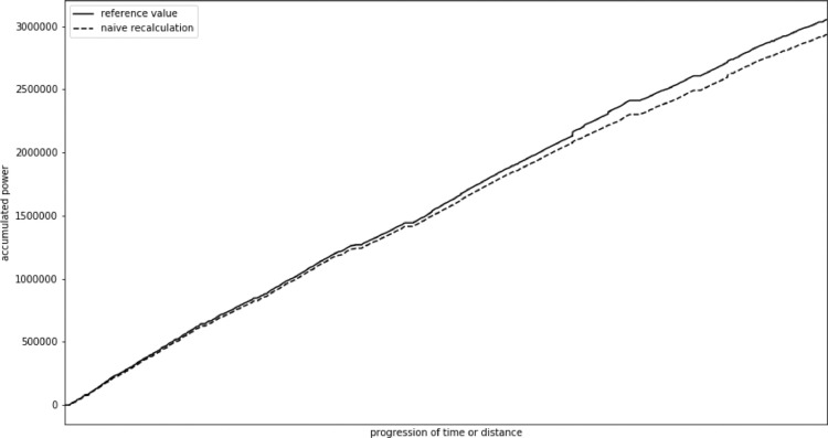
In our study we observed a mean error of 12,824 W, that is 1%–2% of the total value. Maximum error reached 119,243 W, that was 4% of total value. In this case, in contrast to heart rate, the errors usually accumulate. Fig. 2 presents change in accumulated power value recalculated using a naive approach in comparison with the actual value for an example participant. The change mostly accumulates through the race. We also observed some step changes, especially towards the end of the exercise when cycling speed usually varies more due to exhaustion.
Fig. 2.
Change of accumulated power actual value and naive recalculation.
In the following, an adjusted method for power recalculation will be suggested. The method can also be applied to other types of data that exhibit similar recalculation error. When applying this method, the error was 0 for the whole race for each participant. Small variations (< 0.1%) in error occurred in the parts of the race when 1s-long time sections misaligned with 10m-long distance sections. These errors decrease with a growing segment length, but they could become more pronounced with a growing average cycling speed. Should the average speed reach or exceed 10 m/s, we recommend decreasing distance sampling to once every 20 m to preserve precision. More detailed analysis in distance domain at high velocities might not be feasible with currently available PMDs, since they record data with maximum sampling rate of 1 Hz.
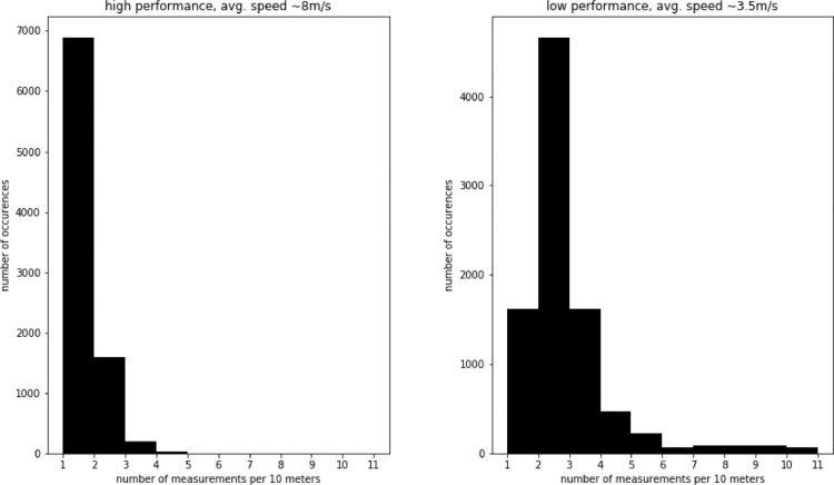
Recalculation must be performed individually for each participant, even though the distance sampling rate is the same for all compared participants. This is due to the large influence of physical fitness on cycling velocity. In Fig. 3 we present histograms of recorded values per 10 m for an example comparing a high (fast)- with a lower (slower) performance participant. In this example, performance was defined as the total time it took each participant to complete the race. It can be observed that in case of a low-performer, due to lower average speed, there are usually two or more recordings per 10 m. In case of a high performer, due to higher average speed, there is only one recording per 10 m.
Fig. 3.
Histogram of recorded values per 10 m for different types of participants.
In our analysis, a sampling rate of 1 measurement point per 10 m was used, as this distance was equivalent to the average distance covered in one second by the average cyclist studied. Other distance values should be considered for different racing speeds. This way it is also possible to avoid even more complex recalculation approaches that would have to involve changing speed. It is also important to appreciate that a single power value does not carry much meaning. The rolling sum or mean power for 15 to 60 s (approx. 150–600 m) was therefore usually used to assess the physiological effects during the race.
The Algorithm 1 assumes that start- and finishing times corresponds to the beginning and end of part of race. However, in real-life PMD data, it can be hard to accurately identify the start or finish of an exercise segment. Moreover, frequently there is no exact correspondence between data sets at these points. The nearest data points are therefore often used to substitute missing values. In some cases, data are so close to the original start/stop point, that a specific compensation might not be necessary. Therefore, the strategy used to compensate for this approximation may need to be adapted to different situations. In the present study, on an average distance of one-kilometer, errors varied between 0%–0.1%. Therefore, we deemed such compensation unnecessary in practice.
Algorithm 1 Algorithm for recalculation of power values when changing sampling base from time to distance.
| Data: TS:= array of T time-ordered samples [[D, Pacc, HR]t = 1, |
| … |
| [D, Pacc, HR]t = T] |
| Result: DS:= array of D distance-ordered samples [[T, P, HR]d = 1, |
| … |
| [T, P, HR]d = D] |
| 1 round D values in TS to full integers; |
| 2 time at:= list of first of time instances t for each group of identical D values in TS; |
| 3 DS:= list of means of Pacc, HR for each group of identical D values in TS; |
| 4 DS.T:= time.at; |
| 5 resample DS to 1 m; |
| 6 interpolate all columns in DS; |
| 7 resample DS to 10 m; |
| 8 DS.P:= DS.Pacc - shift(DS.Pacc, 1); |
Input data is an array of distance, accumulated power, and heart rate for each time instance t for total time T.
In Line 1 all D distance values were rounded to full meters. Such an operation should preferably be performed for the whole set of variables in a vectorized way. The following lines 2–8 should also be implemented that way. There are vectorized operation available in Python Pandas DataFrames and R's DataFrames. In MATLAB it can be implemented as matrix operations. In principle, it could be replaced with a simple loop if necessary. However, loop implementation exhibits a significantly lower performance. At the same time, presenting these operations as loops would make the above algorithm unnecessarily complicated to read.
In line 2 a new list was created, which groups values with the same distance D and extracts first time instance from each group. As a result, a time series of time instances that correspond to the beginning of each travelled one-meter increment. It is important to notice, that values for some meters would be missing in some participants due to change in speed. This problem is addressed in lines 5–7.
In line 3 the new distance series, that will become the output after all the adjustments, was created. One way of achieving it is by creating same type of groups as in line 2, but this time extracting all values, not just the time variable. In the cases that multiple heart rate and power values exist for a given distance segment, a mean will be calculated. For power measurements this value will later be adjusted. For heart rate the value does not need to be adjusted, as explained earlier. In line 4 the previously calculated time series was inserted as a new column in the distance series DS. This operation had to be performed separately, since it was necessary to identify the starting (or first) time for each distance range. The mean value for each group was calculated for all other variables.
The distance series was resampled to 1 m in line 5. This allows a consistent way to use all the available values. In cases of missing values, the series is interpolated in line 6 and resampled again to 10 m in line 7.
Sampling more frequently than 10 m might result in estimation errors, since usually there are only 1–2 measurements per each 10 m. Temporary resampling to 1 m is used as a tool to avoid skipping values that would not be included in that specific sampling frequency. However, these temporary values are not used for further analysis and are immediately downsampled to 10 m after interpolation is performed.
Finally, instantaneous power values were calculated using accumulated power values in line 8. Two copies of accumulated power column were extracted, and one of them was shifted by one distance period. Subsequently these distance series were subtracted from each other. This operation was specified in a vectorized form, which means that corresponding elements from each list were subtracted. This is equivalent to subtracting previous accumulated power value from current accumulated power value. This provides instantaneous power for the time covered between two consecutive distance points d.
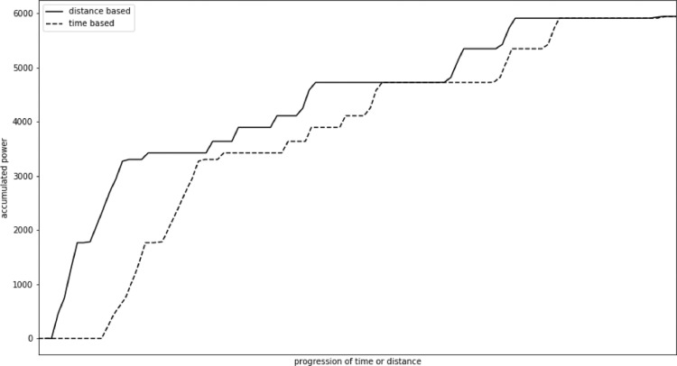
In Fig. 4 it can be observed that accumulated power for time and distance base, merges in the end. This is not the case for the naive recalculation approach. In this figure, the results from the 1-kilometer period of the race with the largest variations in PMD variables, were presented. Power accumulation happens at different relative moments and sometimes at different rates. This is due to the varying speed depending on the race profile, tiredness, and conscious choice by the athlete during the effort. However, the proposed method ensures that the values for any selected distance range will be the same as for the corresponding time range.
Fig. 4.
Change of accumulated power for time and distance base.
Problem 2 - individually adjusting signal range
An assumption of SAX is that signals are within the same range. This assumption is by no means unique to SAX or deep learning. In principle, any modeling method will assume that the meaning of numerical values between various data samples is consistent. If we consider main variables of interest during physical exercise, such as heart rate or power, it might appear that they are within the same range respectively. However, a similar numerical range might be deceiving in this case.
Exercise at an average heart rate of 150 bpm has a completely different impact on a 20-year-old and 60-year-old. For the former, it would be a fairly light exercise in aerobic zone. For the latter, it would be a strenuous anaerobic exercise, close to his maximum heart rate.
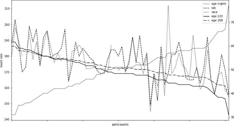
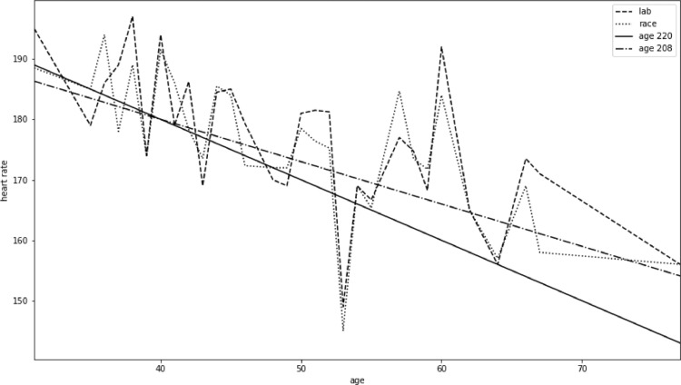
Therefore, to draw correct and consistent conclusions, we need to consider the physiological impact of a measured numerical value. In Figs. 5 and 6 variations in the maximum achievable age adjusted heart rates using four different approaches were compared.
Fig. 5.
Four types of maximum heart rate for each participant.
Fig. 6.
Age and heart rate for all participants.
The conventional way to estimate maximum heart rate is using a formula based on age. Arguably, the most commonly used formula, presented in Eq. (1), uses value of 220 as the base and subtracts age of a person from that value.
| (1) |
Another, maybe less common but more accurate, formula uses 208 as the base and subtracts 0.7 of the person's age. It is presented in Eq. (2). This formula has been extensively tested by Tanaka et al. [11] demonstrating a better correspondence with actual maximum heart rate than the earlier formulas, particularly in older individuals.
| (2) |
Two other approaches to obtaining maximum heart rate rely on data collected under physical load. The simpler approach looks for a maximum value of heart rate across one or many recorded exercises. It is also possible to add a condition on minimum duration in which such value is observed to eliminate outliers or measurement errors. In Eq. (3a) we define a series SHR of heart rate measurement of length T, which corresponds to one participant. The maximum heart rate is then defined in Eq. (3b).
| (3a) |
| (3b) |
| (3c) |
| (3d) |
| (3e) |
| (3f) |
Alternatively, it is also possible to specify a minimum time period (length of subseries) for which value has to be present to be a maximum. In Eq. (3c) a definition of a subseries of S of a given length L was provided. In Eq. (3d) a set of all possible subsequences of S was defined. In Eq. (3e) a minimum value for a subsequence was defined. Finally, in Eq. (3f) a maximum value of HRmax series was defined, present for at least a period of length L as maximum value of all minimums for a set of all possible subsequences S as a domain for the HRsubmin.
The last approach to obtain a maximum heart rate value involves a controlled trial, usually in a laboratory. Individuals run or cycle a standardized protocol until exhaustion and the maximum heart rate is then calculated in a manner similar to the one presented in Eqs. (3a)–(3f). The only difference is that data from the controlled trial are used.
Figs. 4 and 5 compare four types of maximum heart rates obtained using the just outlined methods for 60 participants of varying age and fitness. A general trend of data from laboratory tests seems to follow Eq. (2), but with significant individual variations. Maximum heart rate obtained from race data corresponds closely to data from the cardiopulmonary exercise tests performed in a laboratory.
One aspect, that might influence measurements during exercise is the fitness of the participants. In case of less well trained individuals, insufficient muscular capacity may be the limiting factor for maximal exercise, thereby failing to reach maximum heart rate during exercise.
The maximum values can be used to scale recorded data for each participant. However, currently there is no library in R or Python that would provide such functionality out-of-the-box. Existing libraries assume that scaling levels are the same for all data points. However, for sports data it is necessary to use individualized levels. Therefore, such scaling has to performed with custom code. We present a simple approach to that in Algorithm 2.
Algorithm 2 Algorithm for individual scaling of heart rate values.
| Data: P:= number of participants |
| T:= number of time points (length of exercise) |
| SHR(p,t):= matrix of heart rate for all participants |
| [[S1,1, …, S1,t, …,S1,T] |
| [Sp,1, …, Sp,t, …,Sp,T] |
| [SP,1, …, SP,t, …,SP,T]] |
| HRMAX(p):= list of maximum heart rates for participants |
| [HRMAX(1), …, HRMAX(p), …, HRMAX(P)] |
| Result: SScaledHR(p,t):= matrix of scaled heart rate for all participants |
| [[S1,1, …, S1,t, …,S1,T] |
| [Sp,1, …, Sp,t, …,Sp,T] |
| [SP,1, …, SP,t, …,SP,T]] |
| 1 for participant in range(1..P) do |
| 2 low:= HRMAX(p)/2; |
| 3 high:= HRMAX(p); |
| 4 for t in range(1..T) do |
| 5 SScaledHR(participant, t):= (SHR(participant, t) - low) / (high - low); |
| 6 if SScaledHR(participant, t) ≥ high then SScaledHR(participant, t):= high; |
| 7 if SScaledHR(participant, t) ≤ min then SScaledHR(participant, t):= min; |
| 8 end |
| 9 end |
Input to the algorithm SHR was defined as a two-dimensional matrix, with P amount of rows and T amount of columns. Each row contains all heart rate values for a given participant across the whole activity. Each column contains all heart rate values for a given time-point in all participants.
A list of maximum heart rates HRMAX was generated, containing the individual maximal heart rate value for each participant. This maximal heart rate can be obtained by various methods, some of which were described earlier in this section. The result is presented in a two-dimensional matrix SScaledHR of the same size and organization as the input matrix SHR.
First, in line 1 we specify an iteration covering each participant separately. This way of iterating is important to maintain the right maximum and minimum values, which are calculated in lines 2 and 3. In line 4 we iterate over all time points for the given participant, rescaling values from matrix SHR to SScaledHR.
The actual maximum and minimum values of the scaled data can be different than that obtained from formulas or laboratory tests. In such a case, it is necessary to address the values beyond these extremes. There are in principle two options. As a first alternative, we might allow values to exceed the extremes. It is a good way to convey the information about somebody's performance. But it might negatively influence SAX level selection, since the range of values increases. The other option is to flatten the values, that is to substitute any value that exceed the maximum or is below minimum with the maximum or minimum respectively. This way some information might be lost, but SAX level selection will be more predictable. Final choice will depend on the application and both versions can be used to for different purposes. In the presented algorithm we use the second option in lines 6 and 7.
Usually only the maximum heart rate value is available as a reference point. In this work, 50% of the maximum heart rate during exercise was considered the minimum exercise heart rate. Smaller values seldom occur during strenuous exercise, except for the very beginning (addressed in Section 6). Not pruning smaller values would lead to less effective use of available number range and negatively influence SAX level selection. In some applications choice of minimum and flattening might need to be adjusted. This would require only minimal changes to the algorithm.
This operation could be vectorized in a manner similar to the Algorithm 1. In the present work a non-vectorized version was presented to demonstrate the underling relation between specific single values in the matrix and their scaling. An analogous algorithm can be used for scaling power or other measured values.
Problem 3 - there exist outliers that would negatively influence level selection
In SAX representation cut off values are decided based on statistical distribution of all values in the dataset. If there are large variations within a dataset due to variable physical effort, analyzing sections dataset will result in a better representation with a higher degree of details.
This may be particularly evident at the very start of physical exercise, when the exercise is preceded by a period of rest. Following alterations in exercise intensity, it takes time for the heart rate to reach a value corresponding with the current effort. It is therefore necessary to consider the initiation separately from the rest for the exercise.
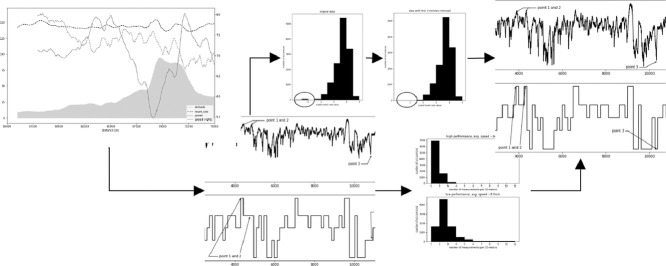
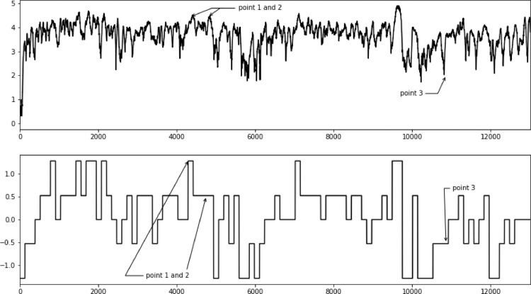
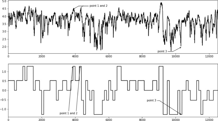
In the top plot in Fig. 7 here is an example of heart rate trajectory of a participant throughout the whole race and in the bottom plot in the same figure a SAX representation of these data. It should be noticed that some points seem to be un- or underrepresented. In case of points 1 and 2 only the first point is properly approximated in the SAX version. Point 3 does not seem to be reflected either.
Fig. 7.
Influence of initial lagged heart rate response on later parts of the race.
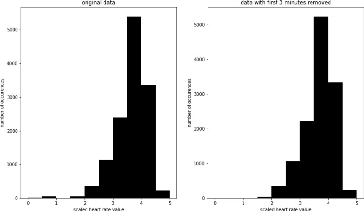
These problems can be greatly reduced by separating the beginning from the rest of the exercise. In the top plot in Fig. 8 we see heart rate development of the same participant, but with first 8 min of the race removed. In the bottom plot of the same figure we see a SAX representation of these data. In this case, all points (1, 2, and 3) are represented in an expected way. In Fig. 9 we compare histograms of scaled values for the whole race and the scaled values with first 8 min of the race removed. There are relatively few values falling in the 0–1 range for the whole race, but as we saw earlier, they have a major impact on the developed model. There are no values in that range after removing the first 8 min.
Fig. 8.
Improved SAX representation after removing first 8 min of the race.
Fig. 9.
Histogram of scale values for the whole race (left) and with first 8 min removed (right).
Depending on the intensity, types of participants, and preceding warm up it would be advisable to separate first 5 to 15 min of the activity. Jeukendrup et al. [12] provide more details explanation and recommendations for addressing this phenomenon, which is known as cardiac drift. The separated part can still be useful for further analysis. For example, the rate of heart rate increase or initial HRV can be indicative of form of the day.
This problem can also impact modeling with LSTM. Deep learning methods are sensitive to data distribution, so the data need to be adequately scaled [[13], [14], [15], [16]]. Outliers will reduce available range for the rest of the data and lead to a worse model. This problem might not be observable in LSTM as easily as in the case of SAX, since the internals LSTM are not easily visualized. Nevertheless, it remains to have impact on the accuracy of the deep model.
Concluding remarks
The analysis of PMD data is challenging. The majority of existing work use cumulative statistics or derivatives directly on the datasets, thereby loosing potential important information from individual data and data interactions.
Some important challenges to PMD data analysis relate to the following problems: (1) the need to preserve data quality when shifting between time and distance bases; (2) the data range varies significantly due to physiological differences between subjects; (3) data exhibits different statistical properties during the course of physical exercise, due to physiological adaptations, leading to lower quality models if not addressed.
In this paper, an algorithm for improved recalculation of measurements when moving between time- and distance bases was presented. While a naive approach can result in errors reaching 4% of the actual value, the presented approach had zero total error and marginal error when applied to subsets of the data.
The present work outlines possible sources of scaling extrema and explains why popular scaling libraries cannot be used in PMD context. A simple algorithm to correctly scale PMD data is presented.
Finally, it was demonstrated that cardiac drift can lead to modeling problems in PMD data. The present work demonstrated that separating out the first 5 to 10 min of an activity (adjusting for warm up and other factors) can lead to improved data modeling.
These three approaches, especially when used together, should enable better analysis of complete datasets from PMDs, rather than having to rely on approaches using cumulative statistics. These approaches allow more effective applications of the established SAX modeling and new deep learning models, such as LSTM.
Declaration of Competing Interest
The authors declare that they have no known competing financial interests or personal relationships that could have appeared to influence the work reported in this paper.
References
- 1.Box G.E., Jenkins G.M., Reinsel G.C., Ljung G.M. John Wiley & Sons; 2015. Time Series Analysis: Forecasting and Control. [Google Scholar]
- 2.Makridakis S., Hibon M. ARMA models and the BoxJenkins methodology. J. Forecast. 1997;16(3):147–163. [Google Scholar]
- 3.Lin J., Keogh E., Wei L., Lonardi S. Experiencing SAX: a novel symbolic representation of time series. Data Min. Knowl. Discov. 2007;15(2):107–144. doi: 10.1007/s10618-007-0064-z. [DOI] [Google Scholar]
- 4.Camerra A., Palpanas T., Shieh J., Keogh E. Proceedings of the IEEE International Conference on Data Mining. IEEE; 2010. iSAX 2.0: indexing and mining one billion time series; pp. 58–67. [Google Scholar]
- 5.Z.C. Lipton, D.C. Kale, C. Elkan, R. Wetzel, Learning to Diagnose with LSTM Recurrent Neural Networks, arXiv: 1511.03677.
- 6.Pathinarupothi R.K., Vinaykumar R., Rangan E., Gopalakrishnan E., Soman K. Proceedings of the IEEE EMBS International Conference on Biomedical & Health Informatics (BHI) IEEE; 2017. Instantaneous heart rate as a robust feature for sleep apnea severity detection using deep learning; pp. 293–296. [Google Scholar]
- 7.Swapna G., Kp S., Vinayakumar R. Automated detection of diabetes using CNN and CNN-LSTM network and heart rate signals. Procedia Comput. Sci. 2018;132:1253–1262. [Google Scholar]
- 8.Zhang Y., Yang Z., Lan K., Liu X., Zhang Z., Li P., Cao D., Zheng J., Pan J. Proceedings of the IEEE INFOCOM 2019-IEEE Conference on Computer Communications Workshops (INFOCOM WKSHPS) IEEE; 2019. Sleep stage classification using bidirectional lstm in wearable multi- sensor systems; pp. 443–448. [Google Scholar]
- 9.Guan Y., Pltz T. Proceedings of the ACM on Interactive, Mobile, Wearable and Ubiquitous Technologies. Vol. 1. 2017. Ensembles of deep LSTM learners for activity recognition using wearables; pp. 1–28. [Google Scholar]
- 10.Lin J., Keogh E., Lonardi S., Chiu B. A symbolic representation of time series, with implications for streaming algorithms. Proceedings of the 8th ACM SIGMOD Workshop on Research Issues in Data Mining and Knowledge Discovery - DMKD ’03; San Diego, California; 2003. p. 2. [DOI] [Google Scholar]
- 11.Tanaka H., Monahan K.D., Seals D.R. Age-predicted maximal heart rate revisited. J. Am. Coll. Cardiol. 2001;37(1):153–156. doi: 10.1016/s0735-1097(00)01054-8. [DOI] [PubMed] [Google Scholar]
- 12.Jeukendrup A., Diemen A.V. Heart rate monitoring during training and competition in cyclists. J. Sports Sci. 1998;16(sup1):91–99. doi: 10.1080/026404198366722. [DOI] [PubMed] [Google Scholar]
- 13.Salimans T., Kingma D.P. Proceedings of the Advances in Neural Information Processing Systems. 2016. Weight normalization: a simple reparame- terization to accelerate training of deep neural networks; pp. 901–909. [Google Scholar]
- 14.Amari S.-I. Proceedings of the Advances in Neural Information Processing Systems. 1997. Neural learning in structured parameter spaces-natural Rie- Mannian gradient; pp. 127–133. [Google Scholar]
- 15.Martens J. Deep learning via hessian-free optimization. ICML. 2010;27:735–742. [Google Scholar]
- 16.Martens J., Grosse R. Proceedings of the International Conference on Machine Learning. 2015. Optimizing neural networks with Kronecker-factored approximate curvature; pp. 2408–2417. [Google Scholar]
- 17.Banaee H., Ahmed M.U., Loutfi A. A framework for automatic text generation of trends in physiological time series data. Proceedings of the IEEE International Conference on Systems, Man, and Cybernetics; Manchester; 2013. pp. 3876–3881. [DOI] [Google Scholar]
- 18.Oates T. Exploiting representational diversity for time series classification. Proceedings of the 11th International Conference on Machine Learning and Applications; Boca Raton, FL, USA; 2012. pp. 538–544. [DOI] [Google Scholar]
- 19.Milanko S., Jain S. LiftRight: quantifying strength training performance using a wearable sensor. Smart Health. 2020 doi: 10.1016/j.smhl.2020.100115. [DOI] [Google Scholar]
- 20.Lai G., Chang W.-.C., Yang Y., Liu H. Modeling long- and short-term temporal patterns with deep neural networks. Proceedings of the 41st International ACM SIGIR Conference on Research & Development in Information Retrieval - SIGIR ’18; Ann Arbor, MI, USA; 2018. pp. 95–104. [DOI] [Google Scholar]
- 21.P. Malhotra, L. Vig, G. Shroff, and P. Agarwal, “Long Short Term Memory Networks for Anomaly Detection in Time Series,” in Proceedings, 2015, vol. 89.
- 22.Bjørkavoll-Bergseth M. Duration of elevated heart rate is an important predictor of exercise-induced troponin elevation. J. Am. Heart Assoc. 2020;9(4) doi: 10.1161/JAHA.119.014408. [DOI] [PMC free article] [PubMed] [Google Scholar]


