On the role of governmental action and individual reaction on COVID-19 dynamics in South Africa: A mathematical modelling study

Abstract

Mathematical models proffer a rational basis to epidemiologists and policy makers on how, where and when to control an infectious disease. Through mathematical models one can explore and provide solutions to phenomena which are difficult to measure in the field. In this paper, a mathematical model has been used to explore the role of government and individuals reaction to the recent outbreak of severe acute respiratory syndrome coronavirus 2 (SARS-CoV-2). The proposed framework incorporates all the relevant biological factors as well as the effects of individual behavioral reaction and government action such as travel restrictions, social distancing, hospitalization, quarantine and hygiene measures. Understanding the dynamics of this highly contagious SARS-CoV-2, which at present does not have any therapy assist the policy makers on evaluating the effectiveness of the control measures currently being implemented. Moreover, policy makers can have insights on short-and-long term dynamics of the disease. The proposed conceptual framework was combined with data on cases of coronavirus disease (COVID-19) in South Africa, March 2020 to early May 2020. Overall, our work demonstrated optimal conditions necessary for the infection to die out as well as persist.

Highlights

• •A conceptual model to investigate the transmission and control of Coronavirus (COVID-19) in South Africa has been considered.
• •All currently know and relevant biological features of the disease have been included in the model.
• •The model is fitted with COVID-19 dataset for South Africa.
• •Effects of government action and individual reaction have been evaluated.
• •Threshold levels for disease eradication and persistence have been determined.

1. Introduction

In late December 2019, a novel strand of Coronavirus (SARS-CoV-2) was reported in Wuhan, a central and crowded city of China (Li et al., 2020). Subsequently, the World Health Organization (WHO) has since officially termed this pandemic the Corona Virus Disease 2019 (COVID-19) [1]. COVID-19 is a rapidly spreading infectious disease and continues to cause several outbreaks in multiple world countries. As of April 12, 2020 (08:00 GMT+2), COVID-19 had resulted in 3,146,651 confirmed cases, 218,178 deaths, 961,833 recoveries, in 213 nations, areas and territories [2].

The public panic in face of the ongoing COVID-19 outbreak reminds us the history of the 1918 influenza pandemic, which killed approximately 50–100 million people worldwide [3]. Moreover, its characteristics of mild symptoms in most cases and short serial interval (i.e., 4–5 days) are synonymous to that of the 1918 influenza, rather than the two other coronaviruses (severe acure respiratory syndrome coronavirus, SARS-CoV, and Middle East respiratory syndrome coronavirus, MERS-CoV) [4]. Moreover, since there is neither a vaccine nor treatment (as of April 2020) to control the spread of the disease, measures such as case isolation, contact tracing and quarantine, social distancing and hygiene measures-which were used to mitigate the 1918 influenza are currently being implemented.

Considering the social and economic impact the disease has caused within the shortest period of time, it is therefore prudent to evaluate the strength of the aforementioned intervention strategies to curb the spread of the disease. Various techniques and methods can be used to explore the impact of the current ongoing mitigation strategies. There are various tools and techniques available which predict the dynamics of the disease transmission and also suggest suitable control interventions. Among them, mathematical modeling, analysis and simulation has been found to be a very successful guiding tool that could give a sound direction to policy makers and public health administration on how to effectively prevent and control disease and has been extensively used [5]. With the aid of mathematical models one can be able to infer, understand and proffer solutions to phenomena which are difficult to measure in the field.

Since the outbreak of COVID-19 a number of mathematical models have been proposed, see, for example [4,[6], [7], [8], [9], [10]], to mention but a few. Gilbert and co-workers developed a conceptual model for COVID-19, with a goal to infer the preparedness and vulnerability of different nations. In Kucharski et al. [12] a stochastic transmission model to assess the early transmission and control of COVID-19 in Wuhan was presented. One of the key results from their study was that the decline in COVID-19 cases late January 2020 was due to the introduction of travel control measures. In Lin et al. [4] a general mathematical model for the coronavirus disease 2019 (COVID-19) outbreak in Wuhan, China with individual reaction and governmental action was presented. Although Lin and Co-workers did not fit their framework with data, their work demonstrated the role of individual reaction and governmental action on transmission and control of COVID-19. Motivated by the work of Lin and Co-workers, we proposed a mathematical model for transmission and control of COVID-19 in South Africa. As in Lin et al. [4], the proposed framework incorporates individual reaction and governmental action. However, our framework is unique from that of Lin et al. [4] in that we incorporated six infectious classes, latent stage, symptomatic severe patients, symptomatic mild patients, asymptomatic patients and detected patients, whereas in Lin and Co-workers had only three infectious compartments. We argue that these additional classes clearly present the dynamics of COVID-19 in South Africa and the greater part of the world. For example, as more knowledge about COVID-19 continues to emerge, the role of asymptomatic patients on transmission and control of the disease has become one of the important topic. Zou et al. [13] report that the viral load of asymptomatic patients was similar to symptomatic patients indicating a transmission potential of asymptomatic patients. Hence there is need to infer on the role asymptomatic patients play on COVID-19 dynamics.

2. Material and methods

2.1. Epidemiological model

In this section we present the conceptual framework for modelling COVID-19 outbreak in South Africa. We constructed an ordinary differential equations model that considers the human population subdivided into compartments based upon infection status. Furthermore, the proposed frame work incorporates the effects of individual reaction as well as the government action. Precisely, the model has been formulated based on the following assumptions:

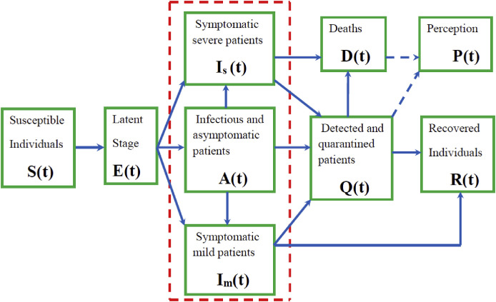
• (i)Vital dynamics (birth rate and natural mortality rate) are not essential, since we are interested on investigating the dynamics of the disease over a very short time frame. The total human population at time t, $N\left(t\right)$ comprise of: susceptible population $S\left(t\right)$-these are individuals who are yet to contract the disease but can do upon exposure to the infection; exposed/latently infected individuals $E\left(t\right)$-these are individuals who have contracted the infection but are not yet infectious, in other words, they are incubating the disease; undetected asymptomatic patients $A\left(t\right)$-these are individuals who would have completed their incubation period and can now transmit the infection. In general, these individuals cannot be recognized if they are not confirmed by RT-PCR or other laboratory testing [14]. The model also includes undetected clinically infected individuals and this population has been further subdivided into two different classes-mild patients $I_m\left(t\right)$ and severe patients $I_s\left(t\right).$ In a recent study by Wu and McGoogan [15], it was noted that approximately 81% of the detected COVID-19 patients were of mild symptom and the remainder (about 20%) were severe. In addition, we have also included detected and quarantined patients (both asymptomatic and symptomatic) $Q\left(t\right)$; as well as the deceased and successfully recovered individuals and these are respectively denoted by $D\left(t\right)$ and $R\left(t\right).$ The population of removed individuals represents individuals who have successfully recovered from infection ‘naturally’ or through ‘treatment’. Thus, the total population is $N\left(t\right)=S\left(t\right)+E\left(t\right)+A\left(t\right)+I_m\left(t\right)+I_s\left(t\right)+Q\left(t\right)+R\left(t\right)+D\left(t\right).$
• (ii)As in He et al. [3] and Lin et al. [4], we assume that the public's perception regarding the number of confirmed cases and deceased influences the dynamics of the disease, hence we have have captured this aspect by including an additional compartment to our framework and this compartment is denoted by $P\left(t\right).$ (iii) Susceptible individuals are assumed to acquire infection following effective contact with undetected asymptomatic patients $A\left(t\right)$, undetected symptomatic patients with mild symptoms $I_m\left(t\right)$, undetected symptomatic patients with severe symptoms $I_s\left(t\right)$ and detected patients $Q\left(t\right).$ Since the outbreak of the novel coronavirus disease (COVID-19) in December 2019, one of the issues that has received major attention is the transmissibility of the coronavirus from asymptomatic patients to healthy individuals [13,16]. In recent study of Yin and Jin [16], no difference in the transmission rates of coronavirus between symptomatic and asymptomatic patients was observed. Our study is also unique from a number of recently published works in that we have assumed that detected patients can transmit the disease. This assertion is based on several reports which have highlighted that healthcare workers (HCWs) are being infected by COVID-19 [[17], [18], [19]]. On 24 February 2020, during a press conference of the WHO-China Joint Mission on CoVID-19, National Health Commission of the People's Republic of China (NHCPRC) reported that since the outbreak began in December 2019 till that day about 2055 healthcare workers (community/hospital-acquired not to be defined) had been confirmed infected with COVID-19, with 22 (1.1%) deaths [17]. As of April 24, 2020, the Spanish Health Ministry reported that 35, 295 HCWs were infected and this represented 20% of all registered cases of COVID-19 in Spain by that time [19]. In addition, a cross-sectional study conducted in 2 teaching hospitals in the Netherlands between 12 March, 2020 and 16 March 2020, revealed that 6% of HCWs at these two institutions were infected with SARS-CoV2 [18]. Thus, the force of infection $\lambda \left(t\right)$, which represents the rate at which susceptible individuals become infected is expressed as:

$$\lambda \left(t\right)=\beta \left(t\right)\left[\frac{I_s\left(t\right)+A\left(t\right)+I_m\left(t\right)+{\epsilon }_{q}Q\left(t\right)}{N\left(t\right)}\right],$$ (1)

where the parameter ${\epsilon }_q$ is a positive constant and accounts for differential infectivity of the detected and quarantine individuals in relation to the undetected patients. Since these individuals are quarantined and interact with a small susceptible population that mainly constitute of HCWs, we assume that $0<{\epsilon }_q<1$. As suggested in the studies of [13,16] we will assume no difference in transmission rate among all the undetected patients. The parameter $\beta \left(t\right)$ models disease transmission rate and is mathematically expressed as

$$\beta \left(t\right)={\beta }_0[1-\alpha ]{\left[1-\frac{P\left(t\right)}{N\left(t\right)}\right]}^{\kappa }.$$ (2)

Equation (2), incorporates the effects of both individuals' reaction and governmental actions; ${\beta }_0$ is the baseline transmission rate; α $\left(0\le \alpha <1\right)$ is the efficacy of ‘governmental actions’ (lockdown, encouraging use of sanitizers, face masks, social distancing) to reduce contacts among individuals. A value of α close to one implies high efficacy and the reverse is true for values of α close to zero. The term ${\left(1-P/N\right)}^{\kappa }$ captures the effects of public perception of the risk to contract the disease based on severe cases reported. Here, κ is a parameter controlling the strength of the response.

• (iv)Susceptible individuals who contract the disease progress to the exposed/latent stage where they will incubate the disease for an average period of ${\sigma }^{-1}$ days. During this period these individuals will not be capable of transmitting the disease. A couple of recent studies on Wuhan COVID-19 dynamics suggest that the average (median) incubation period could be as short as 4 days [4,20].
• (v)Upon the completion of the incubation period, we assume that a fraction f of the exposed individuals move to the asymptomatic stage and the remainder $\left(1-f\right)$ become symptomatic. Prior studies suggests that of the individuals who become symptomatic, more often there exists two classes, mild patients and severe patients [4,15]. In particular, in a study on Wuhan COVID-19 dynamics by Wu and McGoogan [15] it was observed that approximately 81% of the cases were mild symptoms (without pneumonia or only mild pneumonia), 14% were severe cases with difficulty breathing, and 5% were critical with respiratory failure, septic shock, and/or multiple organ dysfunction or failure. Based on this assertion, we assume that a proportion $\left(1-f\right)p$ of exposed individuals progress to infectious stage with mild symptoms and the complementary proportion $\left(1-f\right)\left(1-p\right)$ will become severe.
• (vi)A fraction $\left(1-p_1\right)$ of infectious individuals with mild symptoms are assumed to successfully recover from infection after an average period of ${\gamma }^{-1}$ days and the remainder $p_1$ join the class Q. For severely and critically infected individuals, it is assumed that a fraction $p_2$ enter the class Q after an average duration of ${\delta }^{-1}$ days and the remainder $\left(1-p_2\right)$ succumb to disease-related death. Thus, ${\gamma }^{-1}$ and ${\delta }^{-1}$, represents the mean infectious period of mild and severe patients, respectively. Some prior studies suggests a mean infectious period of 4 days [4].
• (vii)Through RT-PCR or other laboratory testing, asymptotic patients are assumed to be detected and quarantined at rate $\omega .$ Furthermore, we assume that after an average period of ${\varphi }^{-1}$ days, asymptomatic patients will begin to display clinical signs of the disease, with a proportion θ showing mild symptoms and the remainder $\left(1-\theta \right)$ severe. Detected individuals are assumed to exit this class either through successful recovery at rate $\left(1-p_3\right)\eta$ or death at rate $p_3\eta$, ${\eta }^{-1}$ represents the average period one stays in the quarantine stage and $p_3$ denotes a proportion of the quarantined patients who will suffer disease-related death.
• (viii)The public's perception of risk to COVID-19 increases when the number of confirmed COVID-19 cases increases as well as the increase in deaths for quarantined individuals. It is assumed to decay naturally, implying that the perception of risk diminishes over time in the absence of COVID-19 severe and critical cases and deaths. In the proposed model, ${\lambda }^{-1}$ models the mean duration of impact of COVID-19 severe and critical cases and deaths on public perception.

Based on the aforementioned assumptions we have the following system of nonlinear ordinary differential equations:

$$\begin{array}{lll}S\text{′}\left(t\right)\hfill & =\hfill & -\lambda \left(t\right)S\left(t\right),\hfill \\ E\text{′}\left(t\right)\hfill & =\hfill & \lambda \left(t\right)S\left(t\right)-\sigma E\left(t\right),\hfill \\ A\text{′}\left(t\right)\hfill & =\hfill & \sigma fE\left(t\right)-\left(\varphi +\omega \right)A\left(t\right),\hfill \\ I_m\text{′}\left(t\right)\hfill & =\hfill & \sigma \left(1-f\right)pE\left(t\right)+\theta \varphi A\left(t\right)-\gamma I_m\left(t\right),\hfill \\ I_s\text{′}\left(t\right)\hfill & =\hfill & \sigma \left(1-f\right)\left(1-p\right)E\left(t\right)+\left(1-\theta \right)\varphi A\left(t\right)-\delta I_s\left(t\right),\hfill \\ Q\text{′}\left(t\right)\hfill & =\hfill & p_1\gamma I_m\left(t\right)+p_2\delta I_s\left(t\right)+\omega A\left(t\right)-\eta Q\left(t\right),\hfill \\ R\text{′}\left(t\right)\hfill & =\hfill & \left(1-p_1\right)\gamma I_m\left(t\right)+\left(1-p_3\right)\eta Q\left(t\right),\hfill \\ D\text{′}\left(t\right)\hfill & =\hfill & \left(1-p_2\right)\delta I_s\left(t\right)+p_3\eta Q\left(t\right),\hfill \\ P\text{′}\left(t\right)\hfill & =\hfill & p_1\gamma I_m\left(t\right)+p_2\delta I_s\left(t\right)+\omega A\left(t\right)+p_3\eta Q\left(t\right)-\lambda P\left(t\right).\hfill \end{array}\}$$ (3)

Fig. 1 illustrates the transition of individuals from one epidemiological state to another.

Fig. 1.

Model structure. The three compartments $I_s\left(t\right)$, $A\left(t\right)$ and $I_m\left(t\right)$, encompassed by the red-box are undetected infectious populations. (For interpretation of the references to colour in this figure legend, the reader is referred to the Web version of this article.)

2.2. The basic reproduction number

The basic reproduction number, often denoted by ${\mathcal{R}}_0$ is an important threshold parameter for epidemiological models. It is defined as the expected number of secondary cases generated in a completely susceptible population, by one infectious individual during his/her entire infectious period. For models with forward bifurcation, if this metric is less than unity it implies that the infection will die out in the community. However, if it is greater than unity then the disease persists. Although there are several ways of deriving this parameter, the next-generation matrix technique [21,22] is the most popular. One can easily verify that in the absence of the disease, model system (3) admits a trivial equilibrium point, commonly known as the disease-free equilibrium and is given by $S=N,$ $E=A=I_s=I_m=Q=R=D=P=0.$ Utilizing the notation in Ref. [21], the nonnegative matrix F that denotes the generation of new infection terms and the non-singular matrix $V\left(t\right)$ that denotes the remaining transfer terms are respectively given (at the disease-free equilibrium) by;

$$\text{F}=\left[\begin{array}{lllll}0\hfill & {\beta }_0\left(1-\alpha \right)\hfill & {\beta }_0\left(1-\alpha \right)\hfill & {\beta }_0\left(1-\alpha \right)\hfill & {\beta }_0{\epsilon }_q\left(1-\alpha \right)\hfill \\ 0\hfill & 0\hfill & 0\hfill & 0\hfill & 0\hfill \\ 0\hfill & 0\hfill & 0\hfill & 0\hfill & 0\hfill \\ 0\hfill & 0\hfill & 0\hfill & 0\hfill & 0\hfill \\ 0\hfill & 0\hfill & 0\hfill & 0\hfill & 0\hfill \end{array}\right],$$

$$V=\left[\begin{array}{lllll}\sigma \hfill & 0\hfill & 0\hfill & 0\hfill & 0\hfill \\ -\sigma f& \omega +\varphi & 0& 0& 0\\ -\sigma fp& -\theta \varphi \hfill & \gamma \hfill & 0\hfill & 0\hfill \\ -\sigma f\left(1-p\right)& -\left(1-\theta \right)\varphi \hfill & 0\hfill & \delta \hfill & 0\hfill \\ 0\hfill & -\omega \hfill & -p_1\gamma \hfill & -p_2\delta \hfill & \eta \hfill \end{array}\right].$$

It follows that the spectral radius of model (3) which is the reproduction number of the model is given by

$${\mathcal{R}}_{\text{eff}}={\mathcal{R}}_a+{\mathcal{R}}_s+{\mathcal{R}}_m+{\mathcal{R}}_q,$$ (4)

where ${\mathcal{R}}_a$, ${\mathcal{R}}_s$, ${\mathcal{R}}_m$ and ${\mathcal{R}}_q$, represents the contribution of undetected asymptomatic patients, undetected symptomatic patients with severe symptoms, undetected symptomatic patients with mild symptoms and quarantined patients, respectively, on the generation of secondary infections, and they are defined as follows

$$\begin{array}{lll}{\mathcal{R}}_a\hfill & =\hfill & \frac{{\beta }_0\left(1-\alpha \right)f}{\varphi +\omega },\hfill \\ {\mathcal{R}}_s\hfill & =\hfill & \frac{{\beta }_0\left(1-\alpha \right)f}{\delta }\left[\left(1-p\right)+\frac{\left(1-\theta \right)\varphi }{\varphi +\omega }\right],\hfill \\ {\mathcal{R}}_m\hfill & =\hfill & \frac{{\beta }_0\left(1-\alpha \right)f}{\delta }\left[p+\frac{\theta \varphi }{\varphi +\omega }\right],\hfill \\ {\mathcal{R}}_q\hfill & =\hfill & \frac{{\beta }_0{\epsilon }_q\left(1-\alpha \right)f}{\eta }\left[p_1\left\{p+\frac{\left(\omega +p_1\theta \varphi \right)}{p_1\left(\varphi +\omega \right)}\right\}+p_2\left\{\left(1-p\right)+\frac{\left(1-\theta \right)\varphi }{\varphi +\omega }\right\}\right].\hfill \end{array}\}$$

From the expression of the reproduction number ${\mathcal{R}}_{\text{eff}}$, we can note the following:

• (i)Increasing the strength of governmental action to high levels (close to 100%), will lead to a huge reduction in the magnitude of the reproduction number, and the weak actions (values of α close to zero) will not be effective to reduce the magnitude of the basic reproduction number.
• (ii)In the absence of governmental actions $\left(\alpha =p_1=p_2=\omega ={\epsilon }_q=0\right)$, the number of secondary cases that will be generated by each infected individual will be higher compared to when actions are even weak. The expression for the reproduction number in the absence of intervention strategies is given by

$${\mathcal{R}}_0=\frac{{\beta }_{0}f\left[\delta +\varphi \left(2-\left(p+\theta \right)\right)\left(1-{\epsilon }_m\right)\right]}{\varphi \delta }.$$

• (iii)We can also observe that if quarantined individuals do not contribute to the generation of new infections, that is, ${\epsilon }_q={\mathcal{R}}_q=0$, then the reproduction number will be less.

3. Results and discussions

3.1. Data acquisition and disease parameter estimation

We present an application of our model to a case study of South Africa. We use the COVID-19 data for South Africa released and updated by the South African government authorities available on www.worldometer.com [23]. The dataset has also been included in the appendix. The data presented in the appendix starts from the 5th of March 2020 when South Africa reported its first case of COVID-19 case imported from Italy one of the global hotspots of the pandemic. However, when fitting our model, we considered the data ranging from 26 of March 2020 to 3 May 2020, when the lockdown started in South Africa. This was necessitated by the need to exclude the effects of imported cases. Furthermore, we assume that by this date our framework will be able to capture the effects of local transmission since it was now the time of the lockdown. Overall, the data in the appendix suggests that with increasing testing and screening of possible COVID-19 infected individuals, the reported detected cases continue to rise with time indicating the prevalence of COVID-19 infection in South Africa might be higher than the current reported cases.

Moreover, the data presented in the appendix reflects the number of confirmed COVID-19 cases during the ongoing lockdowns and will be used to estimate our unknown model parameters not currently available in literature. Much information remains unknown regarding COVID-19 infection and more work is being done by experts from across the multi-disciplinary facets of research to provide answers to some unknown information on COVID-19. However, much effort to unpack these underlying issues of this pandemic is being witnessed to date. Thus, in this work we resort to curve fitting which is a process that allows us to quantitatively estimate the trend of the outcomes of this pandemic. Equations of approximating curves are fit to the raw field data. However, the fitting curves for any given set of data are not unique. Thus, we choose a curve with the minimum possible deviation from all the data points involved. We make use of the least squares curve fit routine (lsqcurvefit) in Matlab with optimization to estimate our unknown model parameters. Estimated model parameters and their 95% confidence intervals are presented in Table 1 . Other parameters values which were drawn from literature are presented in Table 2 .

Table 1.

Estimation of model parameters with 95% confidence interval (CI).

Description	Symbol	95% CI	Baseline value	Source
Baseline disease transmission rate	${\beta }_0$	[0.2189,0.6324]	0.5944 day−1	Fitting
Modification factor	${\epsilon }_q$	$[0.01462,0.3540]$	0.2126	Fitting
Rate of progression from asymptomatic to symptomatic	${\varphi }^{-1}$	$[0.3540,0.6112]$	0.5556 day −1	Fitting
Proportion of exposed individuals who become asymptomatic	f	$[0.1792,0.0315]$	0.2536	Fitting
Detection rate of asymptomatic individuals	ω	$[0.0001,0.00037]$	0.00025 day−1	Fitting
Proportion of mild patients who are detected and quarantined	$p_1$	$[0.1824,0.2337]$	0.2134	Fitting
Proportion of detected and quarantined severe patients	$p_2$	$[0.7162,0.8043]$	0.7536	Fitting
Recovery rate	η	$[0.2862,0.5231]$	0.4345 day−1	Fitting

Table 2.

Baseline values for model parameters obtained from literature.

Description	Symbol	Range	Baseline value	Source
Governmental action strength	α	$0.4239-0.8478$	0.55	[3,4]
Intensity of response	κ	$695.1-2254.1$	1117.3	[3,4]
Mean latent period	${\sigma }^{-1}$	3–5	5 days	[4]
Mean infectious period of mild patients	${\gamma }^{-1}$	4–7	5 days	[4]
Mean infectious period of severe patients	${\delta }^{-1}$	1–18	5 days	[4]
Proportion of exposed individuals who develop mild symptoms	p	$0-0.8$	0.8	[4]
Proportion of asymptomatic cases who become mild	θ	$0-0.8$	0.8	[4]
Mean duration of public reaction	${\lambda }^{-1}$	4.90–21.00	11.2	[3,4]
Proportion of quarantined patients who die	$p_3$	$0.0384-0.0611$	0.04	[11]

We fitted the model to cumulative daily new infection data presented in the appendix. The cumulative new infections predicted by our model, $C\left(t\right)$, are given by the solution (6) of the following equation:

$$C\text{'}\left(t\right)=p_1\gamma I_m\left(t\right)+p_2\delta I_s\left(t\right)+\omega A\left(t\right).$$ (5)

Thus, the estimation of confirmed cumulative cases for COVID-19 over a defined time frame $t_{k-1}\le t\le t_k$ (where $t_{k-1}$ and $t_k$ marks the beginning and end of the time interval, respectively) from the model output requires to compute:

$${\int }_{t_{k-1}}^{t_k}\left[p_1\gamma I_m\left(t\right)+p_2\delta I_s\left(t\right)+\omega A\left(t\right)\right]dt.$$ (6)

The following initial conditions were determined upon fitting the data, $S\left(0\right)=N-E\left(0\right)-A\left(0\right)-I_m\left(0\right)-I_s\left(0\right)-Q\left(0\right)-R\left(0\right)$ where $N=58\times {10}^6$, $E\left(0\right)=3000$, $A\left(0\right)=100$, $I_m\left(0\right)=200$, $I_s\left(0\right)=50$, $Q\left(0\right)=915$, $R\left(0\right)=12$, $D\left(0\right)=0$, $P\left(0\right)=20$. In this study, the term ‘active cases’ as defined by Worldometer refers to the population of individuals who have tested positive to infection but have neither successfully recovered from it nor succumbed to disease-related death.

Using baseline values on Table 1, Table 2 we have noted that the basic reproduction number of model (3) in the absence of government action and individual reaction ${\mathcal{R}}_0$ will be 3.54. However, in the presence of governmental action and individual reaction at 55% efficacy the reproduction number will be ${\mathcal{R}}_{\text{eff}}=1.8.$ It is worth noting that this is baseline value when effectiveness of aforementioned intervention strategies is fixed at 55% efficacy.

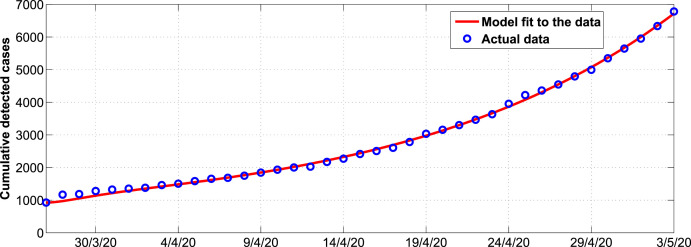
Fig. 2 shows the trends in the cumulative COVID-19 detected cases in South Africa. We observe from Fig. 2, that system (3) fits well with the data from Table 3 (see appendix). Estimated parameter values are shown in Table 1.

Fig. 2.

Model system $\left(3\right)$ fitted to data for cumulative COVID-19 cases in South Africa. The blue circles indicate the actual data and the solid red line indicates the model fit to the data. (For interpretation of the references to colour in this figure legend, the reader is referred to the Web version of this article.)

3.2. Simulation results

To explore the impact of individual reaction and governmental action on combating COVID-19 disease in South Africa, we will simulate model (3) using parameter values in Table 1, Table 2 Majority of these parameter values were adopted from the recently published literature on COVID-19 and the remaining unknown parameters were estimated from data fitting. Estimated parameters are within plausible range of values so as to capture the current COVID-19 transmission dynamics in South Africa. The total population of South Africa in this study was assumed to be 58 million. We perform numerical simulations considering the period when the lockdown was instituted in South Africa, on the 26th of March 2020. At that particular time we assume that there were certain individuals who remained undetected and suit to be classified in one of the following compartments: asymptomatic, mildly infected or severely infected. Also, as reported by the South African government, there were certain individuals who had successfully recovered from the disease.

We aim to intrinsically investigate the impact of asymptomatic infections on the general dynamics of COVID-19. We determine to what extent the current 35 day lockdown in South Africa has been by comparison with the scenario when there was no lockdown instituted.

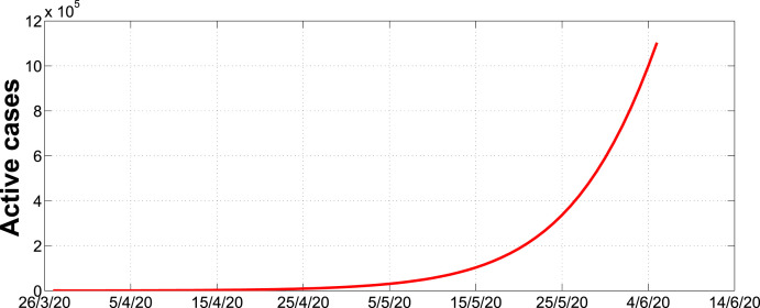
Fig. 3 illustrates how the active cases were going to progress in the absence of lockdown. As shown in the graph, the number of cases were going to increase rapidly more or less in an exponential growth scenario. In particular, the number of cases could be around 100000 beginning of June. However, in Fig. 4 we can observe that in the presence of intervention strategies, the number of infections may not exceed 18,000 cases for the entire 450 day period.

Fig. 3.

Simulation of active cases with no lockdown over a 70 day period.

Fig. 4.

Simulation of active cases during the first 35 day lockdown in stage 5 with successive 14 day, 21 day and 35 day lockdowns in stages 4, 3, 2 and 1 and thereafter partially relaxed.

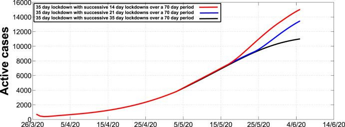
Fig. 5 illustrates the expected number of active cases for different successive lockdown extensions after the initial 35 day lockdown. We consider extensions of 14 day stages, 21 day stages and 35 day stages. We observe that a 14 day extension will result to approximately 15000 cases, a 21 day extension will result to approximately 13000 and a 35 day extension will result to approximately 11000 cases by the 4th of June 2020.

Fig. 5.

Simulation of active cases during the first 35 day lockdown in stage 5 with successive 14 day, 21 day and 35 day lockdowns in stages 4, 3, 2 and 1 and thereafter partially relaxed.

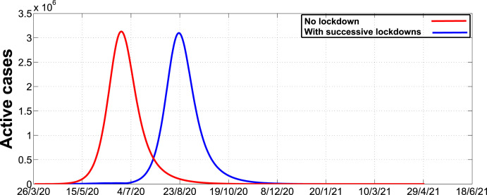
Fig. 6 illustrates the dynamics of the disease in the absence and presence of intervention strategies over a 450 day period. As we can observe, the number of active cases in the absence of intervention strategies will reach a peak around mid-June whereas in the presence of intervention strategies the peak will be attained around the 23rd of August. The results suggests that the presence of intervention strategies may be responsible for the delay in attaining the peak. This may give policy makers ample time to prepare for effective disease management.

Fig. 6.

Simulation of active cases in the absence and presence of successive lockdowns and thereafter fully relaxed.

Fig. 7 indicates that as the detection rate, modelled by ω, increases then the number of active cases decreases. It is important to note that a value of ω between 0.5 and 1.0 may not result in a significant change in the number of active cases. Thus, we recommend that the detection level of 0.5 and above may lead to a remarkable decline in the number of active cases.

Fig. 7.

Effects of varying the detection of asymptomatic infections ω on the number of active cases, starting from 0.0 up to 1.0 with a step size of 0.1 across the given time interval.

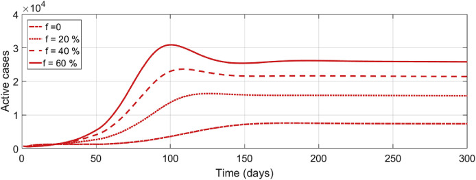
Numerical illustration in Fig. 8 depicts the effects of different levels of exposed individuals who progress to asymptomatic and infectious stage. As we can observe, an increase in the number of these individuals have a significant impact on short-and long-term dynamics of the disease. In particular, for any value of f greater than 20%, then the number of active cases may be greater than 10,000 in 100 days. However, for any value of f less than 20% the number of active cases may not exceed 10000, for the entire 300 day period.

Fig. 8.

Effects of varying the proportion of exposed individuals who progress to the asymptomatic and infectious stage f on the number of active cases, starting from 0.0 up to 0.6 with a step size of 0.2 across the given time interval.

4. Concluding remarks

The present study aimed to investigate the situation of COVID-19 in South Africa in the presence and absence of mitigation measures. A mathematical model that subdivides the total human population based on one's epidemiological status has been developed. The epidemiological classes considered are susceptible, exposed/latent, asymptomatic, infectious with mild symptoms, infectious with severe and critical symptoms, detected and quarantined, recovered and deceased. The proposed conceptual model has an additional compartment that captures the effects of public perception of risk of infection.

Although we have noted that the presence of intervention strategies may reduce the number of infections per unit time, there are optimal thresholds of intervention strategies that can lead to a significant reduction of cases. For instance, an initial 35 day lockdown followed by successive 14 day lockdowns with relaxation may not be as effective as an initial 35 day lockdown followed by successive 35 day lockdowns with relaxation. Furthermore, we observed that a detection rate of at least 0.5 per day may lead to a significant reduction of the number of active cases. In addition, we also noted that in the absence of intervention strategies the peak number of cases could be attained around mid-June whereas in the presence of intervention strategies the peak will be attained around the 23rd of August. Hence, we can deduce that the presence of intervention strategies may be responsible for the delay in attaining the peak, thereby prompting policy makers ample time to prepare for various and effective ways of managing the disease.

The proposed framework could be of significant importance on understanding the transmission and control of COVID-19. However, we acknowledge that there are several aspects of the disease that are yet to be clearly unraveled, for instance, the duration one remains as an asypmtomatic infectious patient is still debatable. In the event that additional information have been found, it can be used to improve the framework.

Funding

The authors received no specific funding for this work.

Availability of data and materials

All data have been included in the manuscript.

Consent for publication

No personal information is used in this study, thus Not Applicable.

Declaration of competing interest

The authors declare that they have no known competing financial interests or personal relationships that could have appeared to influence the work reported in this paper.

Appendix. Dataset

Here, we provide the dataset that was used in the study. All data are publicly available and can be retrieved on www.worldometer.com. We considered the data ranging from 1 March 2020 to 3 May 2020.

Table 3.

Data for COVID-19 cases in South Africa before and during the lockdown

Date	5/3/20	6/3/20	7/3/20	8/3/20	9/3/20	10/3/20	11/3/20	12/3/20
Total cases	1	1	2	3	7	9	13	16
Date	13/3/20	14/3/20	15/3/20	16/3/20	17/3/20	18/3/20	19/3/20	20/3/20
Total cases	24	38	51	62	85	116	150	202
Date	21/3/20	22/3/20	23/3/20	24/3/20	25/3/20	26/3/20	27/3/20	28/3/20
Total cases	240	274	402	554	709	927	1170	1187
Date	29/3/20	30/3/20	31/3/20	1/4/20	2/4/20	3/4/20	4/4/20	5/4/20
Total cases	1280	1326	1353	1380	1462	1505	1585	1655
Date	6/4/20	7/4/20	8/4/20	9/4/20	10/4/20	11/4/20	12/4/20	13/4/20
Total cases	1686	1749	1845	1934	2003	2028	2173	2272
Date	14/4/20	15/4/20	16/4/20	17/4/20	18/4/20	19/4/20	20/4/20	21/4/20
Total cases	2415	2506	2605	2783	3034	3158	3300	3465
Date	22/4/20	23/4/20	24/4/20	25/4/20	26/4/20	27/4/20	28/4/20	29/4/20
Total cases	3635	3953	4220	4361	4546	4793	4996	5350
Date	30/4/20	1/5/20	2/5/20	3/5/20
Total cases	5647	5951	6336	6783

Appendix A. Supplementary data

The following is the Supplementary data to this article:

References

- 1.Zhu N., Zhang D., Wang W. A novel coronavirus from patients with pneumonia in China, 2019. N Engl J Med. 2020 doi: 10.1056/NEJMoa2001017. [DOI] [PMC free article] [PubMed] [Google Scholar]
- 2.World Health Organization Coronavirus disease (COVID-19) pandemic. https://www.who.int/emergencies/diseases/novel-coronavirus-2019?gclid=CjwKCAjw7-P1BRA2EiwAXoPWA_xVOf3xDCMTZupLrLH4WgYYuJeN7TVnJdeOt9WzDZ9qU_ftrz3 C6hoCZ9AQAvD_BwE (Accessed 12 April 2020)
- 3.He D., Dushoff J., Day T., Ma J., Earn D.J. Inferring the causes of the three waves of the 1918 influenza pandemic in England and Wales. Proc R Soc B: Biol Sci. 2013;280(1766):20131345. doi: 10.1098/rspb.2013.1345. [DOI] [PMC free article] [PubMed] [Google Scholar]
- 4.Lin Q., Zhao S., Gao D. A conceptual model for the outbreak of Coronavirus disease 2019 (COVID-19) in Wuhan, China with individual reaction and governmental action. Int J Infect Dis. 2020;93:211–216. doi: 10.1016/j.ijid.2020.02.058. [DOI] [PMC free article] [PubMed] [Google Scholar]
- 5.Egger M., Johnson L., Althaus C. Developing WHO guidelines: time to formally include evidence from mathematical modelling studies. F1000Res. 2017;6:1584. doi: 10.12688/f1000research.12367.2. Published 2017 Aug 29. [DOI] [PMC free article] [PubMed] [Google Scholar]
- 6.Li Q., Med M., Guan X.H. Early transmission dynamics in Wuhan, China, of novel coronavirus–infected pneumonia. N Engl J Med. 2020 doi: 10.1056/NEJMoa2001316. [DOI] [PMC free article] [PubMed] [Google Scholar]
- 7.Riou J., Althaus C.L. Pattern of early human-to-human transmission of Wuhan 2019 novel coronavirus (2019-nCoV), December 2019 to January 2020. Euro Surveill. 2020;25(4):2000058. doi: 10.2807/1560-7917.ES.2020.25.4.2000058. [published correction appears in Euro Surveill. 2020 Feb;25(7):] [DOI] [PMC free article] [PubMed] [Google Scholar]
- 8.Zhong L., Mu L., Li J., Wang J., Yin Z., Liu D. Early prediction of the 2019 novel coronavirus outbreak in the mainland China based on simple mathematical model. IEEE Access. 2020;8:51761–51769. doi: 10.1109/ACCESS.2020.2979599. http://doi: 10.1109/ACCESS.2020.2979599 [DOI] [PMC free article] [PubMed] [Google Scholar]
- 9.Zhou T., Liu Q., Yang Z. Preliminary prediction of the basic reproduction number of the Wuhan novel coronavirus 2019-nCoV. Evid Base Med. 2020;13(1):3–7. doi: 10.1111/jebm.12376. [DOI] [PMC free article] [PubMed] [Google Scholar]
- 10.Zhao S., Chen H. Modeling the epidemic dynamics and control of COVID-19 outbreak in China. Quant Biol. 2020:1–9. doi: 10.1007/s40484-020-0199-0. http://doi:10.1007/s40484-020-0199-0 [DOI] [PMC free article] [PubMed] [Google Scholar]
- 11.Pang L., Liu S., Zhang X., Tian T., Zhao Z. Transmission dynamics and control strategies of COVID-19 in Wyhan, China. J Biol Syst. 2020;28(3):1–18. doi: 10.1142/S0218339020500096. [DOI] [Google Scholar]
- 12.Kucharski A.J., Russell T.W., Diamond C. Early dynamics of transmission and control of COVID-19: a mathematical modelling study. Lancet Infect Dis. 2020 doi: 10.1016/S1473-3099(20)30144-4. [DOI] [PMC free article] [PubMed] [Google Scholar]
- 13.Zou L., Ruan F., Huang M. SARS-CoV-2 viral load in upper respiratory specimens of infected patients. N Engl J Med. 2020;382(12):1177–1179. doi: 10.1056/nejmc2001737. https://search.crossref.org/?q=Zou+L%2C+Ruan+F%2C+Huang+M%2C+et+al.+SARS-CoV-2+viral+load+in+upper+respiratory+specimens+of+infected+patients.+N+Engl+J+Med.+2020%3B382%2812%29%3A1177%E2%80%931179 [DOI] [PMC free article] [PubMed] [Google Scholar]
- 14.Nishiura H., Kobayashi T., Miyama T. Estimation of the asymptomatic ratio of novel coronavirus infections (COVID-19) Int J Infect Dis. 2020;94:154–155. doi: 10.1016/j.ijid.2020.03.020. [DOI] [PMC free article] [PubMed] [Google Scholar]
- 15.Wu Z., McGoogan J.M. Characteristics of and important lessons from the Coronavirus disease 2019 (COVID-19) outbreak in China: summary of a report of 72,314 cases from the Chinese center for disease control and prevention. J Am Med Assoc. 2020 doi: 10.1001/jama.2020.2648. [DOI] [PubMed] [Google Scholar]
- 16.Yin G., Jin H. Comparison of transmissibility of coronavirus between symptomatic and asymptomatic patients: reanalysis of the ningbo COVID-19 data. JMIR Public Health Surveill. 2020;6(2) doi: 10.2196/19464. https://publichealth.jmir.org/2020/2/e19464 [DOI] [PMC free article] [PubMed] [Google Scholar]
- 17.World Health Organization Report of the WHO-China Joint mission on coronavirus disease 2019 (COVID-19) 2020. https://www.who.int/docs/default-source/coronaviruse/who-china-joint-mission-on-covid-19-final-report.pdf Available at: [last accessed May 2020]
- 18.Kluytmans-van den Bergh M.F.Q., Buiting A.G.M., Pas S.D. Prevalence and clinical presentation of health care workers with symptoms of coronavirus disease 2019 in 2 Dutch hospitals during an early phase of the pandemic. JAMA Netw Open. 2020;3(5) doi: 10.1001/jamanetworkopen.2020.9673. http://doi:10.1001/jamanetworkopen.2020.9673 [DOI] [PMC free article] [PubMed] [Google Scholar]
- 19.Güell O. EL PAIS; 2020. Spain ranks first for Covid-19 infections among healthcare workers.https://english.elpais.com/spanish_news/2020-04-25/spain-ranks-first-for-covid-19-infections-amonghealthcare-workers.html Retrieved from. [Google Scholar]
- 20.Guan W., Ni Z., Hu Y. Clinical characteristics of 2019 novel coronavirus infection in China. NEJM. 2020 doi: 10.1056/NEJMoa2002032. [DOI] [Google Scholar]
- 21.van-den Driessche P., Watmough J. Reproduction number and sub-threshold endemic equilibria for compartment models of disease transmission. Math Biosci. 2002;180:29–48. doi: 10.1016/S0025-5564(02)00108-6. [DOI] [PubMed] [Google Scholar]
- 22.Diekmann O., Heesterbeek J.A.P., Metz J.A.J. On the definition and the computation of the basic reproduction ratio in models for infectious diseases in heterogeneous populations. J Math Biol. 1990;28:365–382. doi: 10.1007/BF00178324. [DOI] [PubMed] [Google Scholar]
- 23.Worldometers Coronavirus cases. 2020. https://www.worldometers.info/coronavirus/coronavirus-cases/ Online. (accessed 3.05.20.)
Associated Data
This section collects any data citations, data availability statements, or supplementary materials included in this article.
Supplementary Materials
Data Availability Statement