Coarse Graining, Fixed Points, and Scaling in a Large Population of Neurons

Abstract

We develop a phenomenological coarse-graining procedure for activity in a large network of neurons, and apply this to recordings from a population of 1000+ cells in the hippocampus. Distributions of coarse-grained variables seem to approach a fixed non-Gaussian form, and we see evidence of scaling in both static and dynamic quantities. These results suggest that the collective behavior of the network is described by a nontrivial fixed point.

In systems with many degrees of freedom, it is natural to search for simplified, coarse-grained descriptions; our modern understanding of this idea is based on the renormalization group (RG). In its conventional formulation, we start with the joint probability distribution for variables defined at the microscopic scale, and then coarse grain by local averaging over small neighborhoods in space. The joint distribution of coarse-grained variables evolves as we change the averaging scale, and in most cases the distribution becomes simpler at larger scales: macroscopic behaviors are simpler and more universal than their microscopic mechanisms [1–4]. Is it possible that simplification in the spirit of the RG will succeed in the more complex context of biological systems?

The exploration of the brain has been revolutionized over the past decade by methods to record, simultaneously, the electrical activity of large numbers of neurons [5–15]. Here we analyze experiments on 1000+ neurons in the CA1 region of the mouse hippocampus. The mice are genetically engineered to express a protein whose fluorescence depends on the calcium concentration, which in turn follows electrical activity; fluorescence is measured with a scanning two-photon microscope as the mouse runs along a virtual linear track. Figure 1(a) shows a schematic of the experiment, described more fully in Ref. [15]. The field of view is 0.5 × 0.5 mm² [Fig. 1(b)], and we identify 1485 cells that were monitored for 39 min, which included 112 runs along the virtual track. Images are sampled at 30 Hz, segmented to assign signals to individual neurons, and denoised to reveal transient activity above a background of silence [Fig. 2(a)].

FIG. 1.

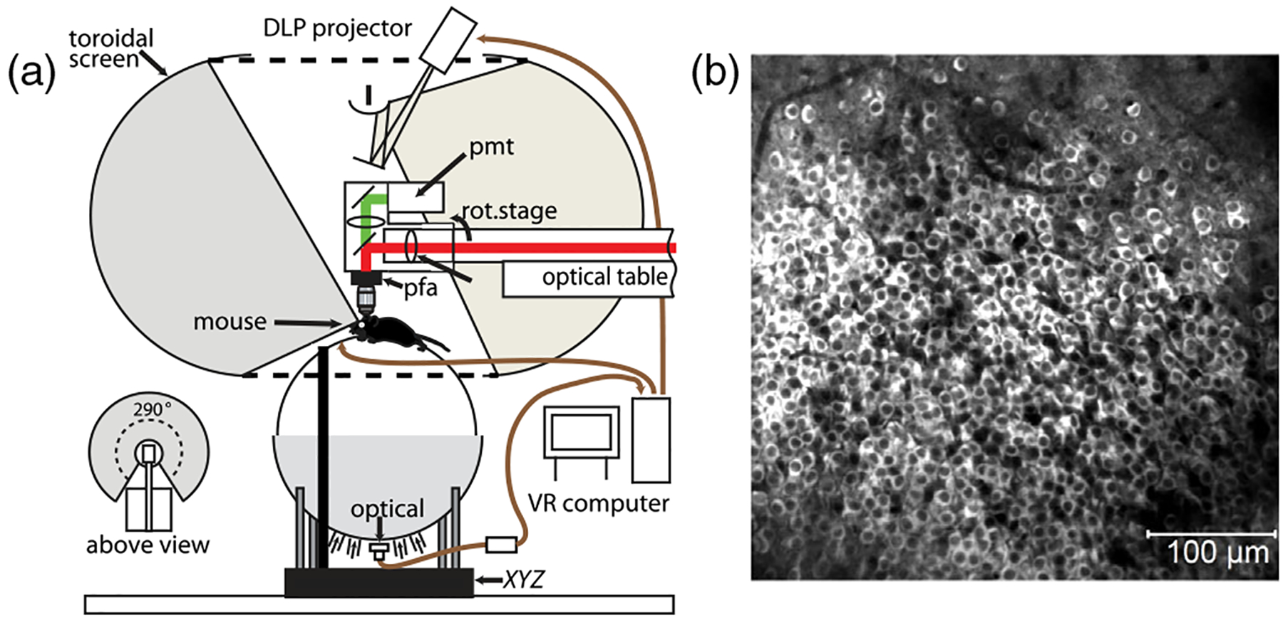
(a) Schematic of the experiment, imaging inside the brain of a mouse running on a styrofoam ball. Motion of the ball advances the position of a virtual world projected on a surrounding toroidal screen. (b) Fluorescence image of neurons in the hippocampus expressing calcium sensitive fluorescent protein.

FIG. 2.

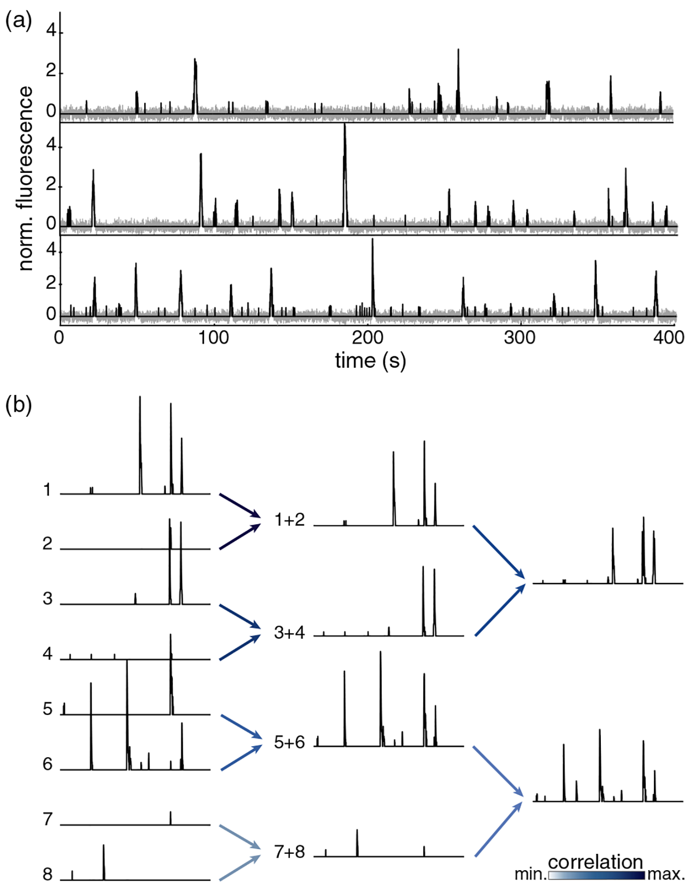
Fluorscence signals, denoising, and coarse graining. (a) Continuous fluorescence signals, raw in grey and denoised in black, for three neurons in our field of view. (b) Activity of eight example neurons. Maximally correlated pairs are grouped together by summing their activity, normalizing so the mean of nonzero values is one. Each cell can only participate in one pair, and all cells are grouped by the end of each iteration. Darker arrows correspond to stronger correlations in the pair.

In familiar applications of the RG, microscopic variables have defined locations in space, and interactions are local, so it makes sense to average over spatial neighborhoods. Neurons are extended objects, and make synaptic connections across distances comparable to our entire field of view, so locality is not a useful guide. But in systems with local interactions, microscopic variables are most strongly correlated with the near spatial neighbors. We will thus use correlation itself, rather than physical connectivity, as a proxy for neighborhood. We compute the correlation matrix of all the variables, search greedily for the most correlated pairs, and define a coarse-grained variable by the sum of the two microscopic variables in the pair [16], as illustrated in Fig. 2. This can be iterated, placing the variables onto a binary tree; alternatively, after k iterations, we have grouped the neurons into clusters of size K = 2^k, and each cluster is represented by a single coarse-grained variable. We emphasize that this is only one of many possible coarse-graining schemes [17].

A technical point concerns the normalization of coarse-grained variables. We start with signals whose amplitude has an element of arbitrariness, being dependent on the relations between electrical activity and calcium concentration, and between calcium concentration and protein fluorescence. Nonetheless, there are many moments in time when the signal is truly zero, representing the absence of activity. We want to choose a normalization that removes the arbitrariness but preserves the meaning of zero, so we set the average amplitude of the nonzero signals in each cell equal to one, and restore this normalization at each step of coarse graining.

Formally, we start with variables describing activity in each neuron {x_i(t)} describing activity in each neuron i= 1,2 ⋯ N at time t; since our coarse graining does not mix different moments in time, we drop this index for now. We compute the correlations

$$c_{ij}=\frac{\langle \delta x_i\delta x_j\rangle }{{\left[\langle {\left(\delta x_i\right)}^2\rangle \langle {\left(\delta x_j\right)}^2\rangle \right]}^{1/2}},$$ (1)

where δx_i = x_i − 〈x_i〉 We then search for the largest nondiagonal element of this matrix, identifying the maximally correlated pair i; j_*(i), and construct the coarse-grained variable

$$x_i^{(2)}=Z_i^{(2)}\left(x_i+x_{j_{*}(i)}\right),$$ (2)

where $Z_i^{(2)}$ restores normalization as described above. We remove the pair [i; j_* (i)] , search for the next most correlated pair, and so on, greedily, until the original N variables have become ⌊N2⌋ pairs. We can iterate this process, generating N_K = ⌊N=K⌋ clusters of size K = 2^k, represented by coarse-grained variables $\left\{x_i^{(K)}\right\}$.

We would like to follow the joint distribution of variables at each step of coarse graining, but this is impossible using only a finite set of samples [18]. Instead, as in the analysis of Monte Carlo simulations [19], we follow the distribution of individual coarse-grained variables. This distribution is a mixture of a delta function exactly at zero and a continuous density over positive values,

$$\begin{gathered} P_K(x)\equiv \frac{1}{N_K}\sum _{i=1}^{N_K}\langle \delta \left(x-x_i^{(K)}\right)\rangle \\ =P_0(K)\delta (x)+\left[1-P_0(K)\right]Q_K(x), \end{gathered}$$ (3)

where our choice of normalization requires that

$${\int }_0^{\infty }dx{Q}_K(x)x=1.$$ (4)

If the coarse-grained activity of a cluster is zero, all the microscopic variables in that cluster must be zero, so that P₀(K) measures the probability of silence in clusters of size K. This probability must decline with K, and in systems with a finite range of correlations this decline is exponential at large K, even if individual neurons differ in their probability of silence.

Figure 3 shows the behavior of P₀ (K) and Q_K (x) from the microscopic scale K = 1 to K = 256 and we see that the data are described, across the full range of K, by

$$P_0(K)=\text{exp}\left(-a{K}^{\tilde{\beta }}\right),$$ (5)

with $\tilde{\beta }=0.87\pm 0.03$ [20]. This scaling with $\tilde{\beta }<1$ suggests that correlations among neurons are self-similar across ~2.5 decades in K [21].

FIG. 3.

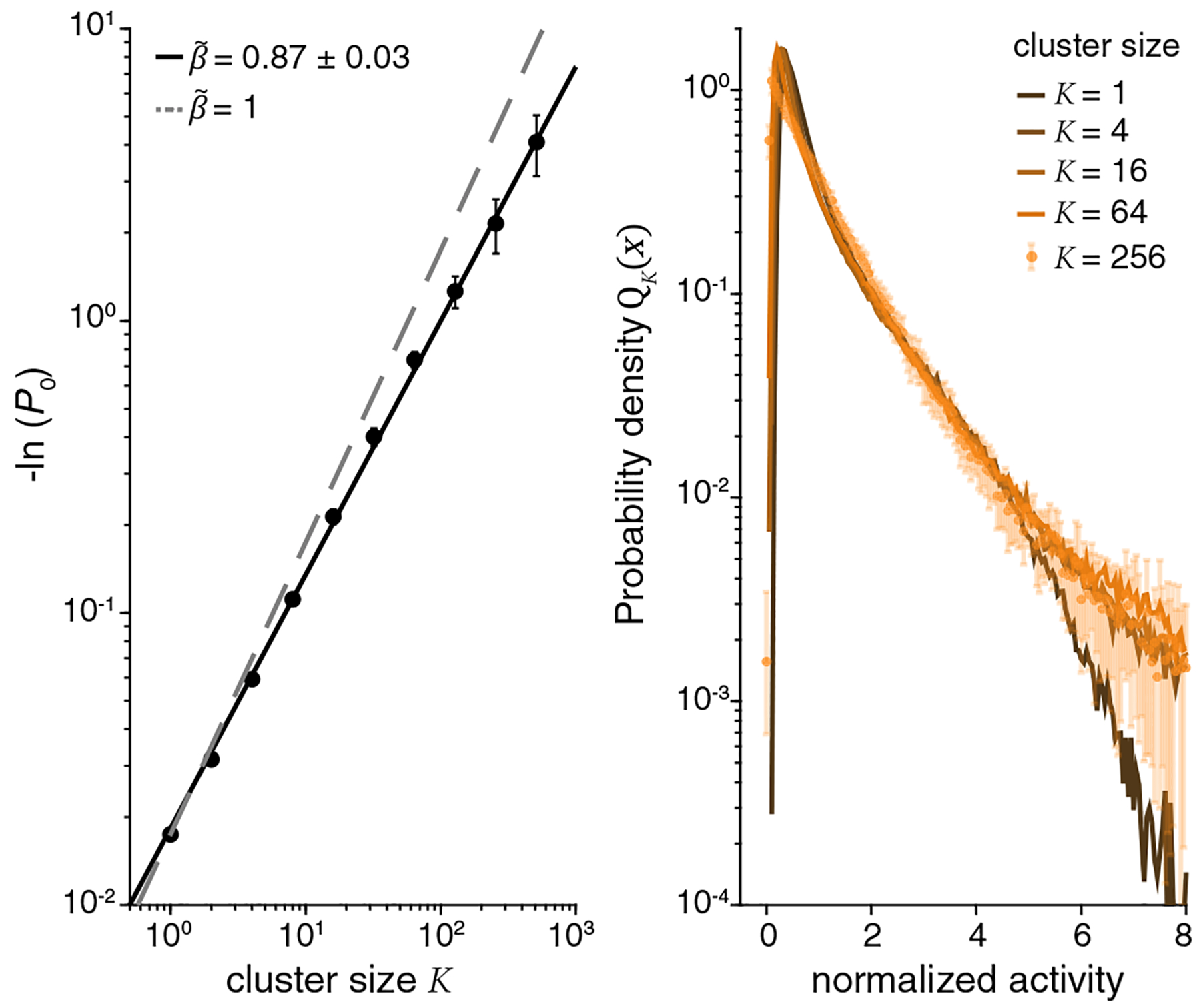
Scaling in the probabilities of silence and activity. (left) Probability of silence as a function of cluster size. Dashed line is an exponential decay $\tilde{\beta }=1$, and the solid line is Eq. (5). (right) Distribution of activity at different levels of coarse graining, from Eq. (3) with normalization from Eq. (4). Larger clusters corresponds to lighter colors.

Coarse graining replaces individual variables by averages over increasingly many microscopic variables. If correlations among the microscopic variables are sufficiently weak, the central limit theorem drives the distribution toward a Gaussian; a profound result of the RG is the existence of non-Gaussian fixed points. While summation of correlated variables easily generates non-Gaussian distributions at intermediate K, there is no reason to expect the approach to a fixed non-Gaussian form, as we see with Q_K(x) on the right side in Fig. 3.

If correlations are self-similar, then we should see this in more detail by looking inside the clusters of size K, which are analogous to spatially contiguous regions in a system with local interactions. We recall that, in systems with translation invariance, the matrix of correlations among microscopic variables is diagonalized by a Fourier transform, and that the eigenvalues λ of the covariance matrix are the power spectrum or propagator G(k) [22]. At a fixed point of the RG this propagator will (be scale invariant, λ = G(k) = A/k^2−η, where the wave vector k indexes the eigenvalues from largest (at small k) to smallest (at large k), and in d dimensions the eigenvalue at k is of rank ~(Lk)^d, where L is the linear size of the system. The number of variables in the system is K ~ (L/a)^d, where a is the lattice spacing and the largest k ~ 1/a. Putting these factors together we have

$$\lambda =B{\left(\frac{K}{\text{rank}}\right)}^{\mu },$$ (6)

with μ = (2 – η)/d. Thus scale invariance implies both a power-law dependence of the eigenvalue on rank and a dependence only on fractional rank (rank/K) when we compare systems of different sizes.

Figure 4 shows the eigenvalues of the covariance matrix, C_ij = 〈δx_iδx_j〉, in clusters of size K = 16, 32, 64, 128; the eigenvalue spectrum of a covariance matrix is distorted by finite sample size, catastrophically so at large K, and we stop at K = 128 to avoid these problems. A power-law dependence on rank is visible (with μ = 0.71 ± 0.15), albeit at only over a little more than one decade; more compelling is the dependence of the spectrum on relative rank, accurate over much of the spectrum within the small error bars of our measurements.

FIG. 4.

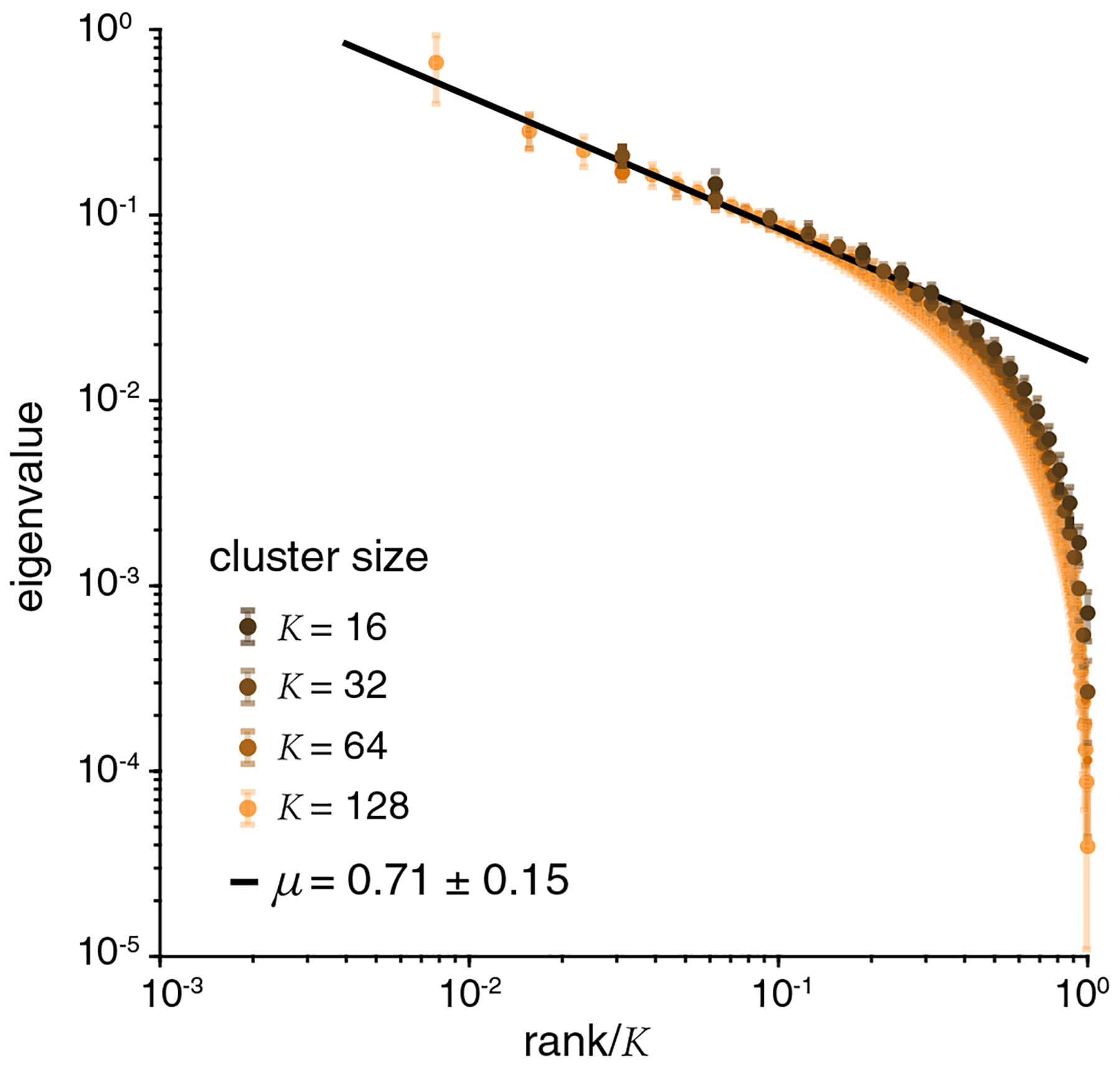
Scaling in eigenvalues of the covariance matrix spectra, C_ij = 〈δx_iδx_j〉, for clusters of different sizes. Larger cluster corresponds to lighter color. Solid line is the fit to Eq. (6).

If we are near a fixed point of the RG, then in systems with local interactions we will see dynamic scaling, with fluctuations on length scale $\mathcal{l}$ relaxing on timescale $\tau \propto {\mathcal{l}}^z$. Although interactions in the neural network are not local, we have clustered neurons into blocks based on the strength of their correlations, and we might expect that larger blocks will relax more slowly. To test this, we compute the temporal correlation functions

$$C_K(t)=\frac{1}{N_K}\sum _{i=1}^{N_K}\langle \delta x_i^{(K)}\left(t_0\right)\delta x_i^{(K)}\left(t_0+t\right)\rangle .$$ (7)

Qualitatively, the decay of C_K(t) is slower at larger K, but we see in Fig. 5 that correlation functions at different K have the same form within error bars if we scale the time axis by a correlation time τ_c(K), which we can define as the 1/e point of the decay. Although the range of τ_c is small (as a result of the small value of $\tilde{z}$), we see that

$${\tau }_c(K)={\tau }_1{K}^{\tilde{z}},$$ (8)

except for the smallest K where the dynamics are limited by the response time of the fluorescent indicator molecule itself; quantitatively, $\tilde{z}=0.11\pm 0.01$. Error bars on τ_c at K = 256 are large; hence we fit up to K = 128; errors at different K are necessarily correlated, which results in relatively small error bars for $\tilde{z}$.

FIG. 5.

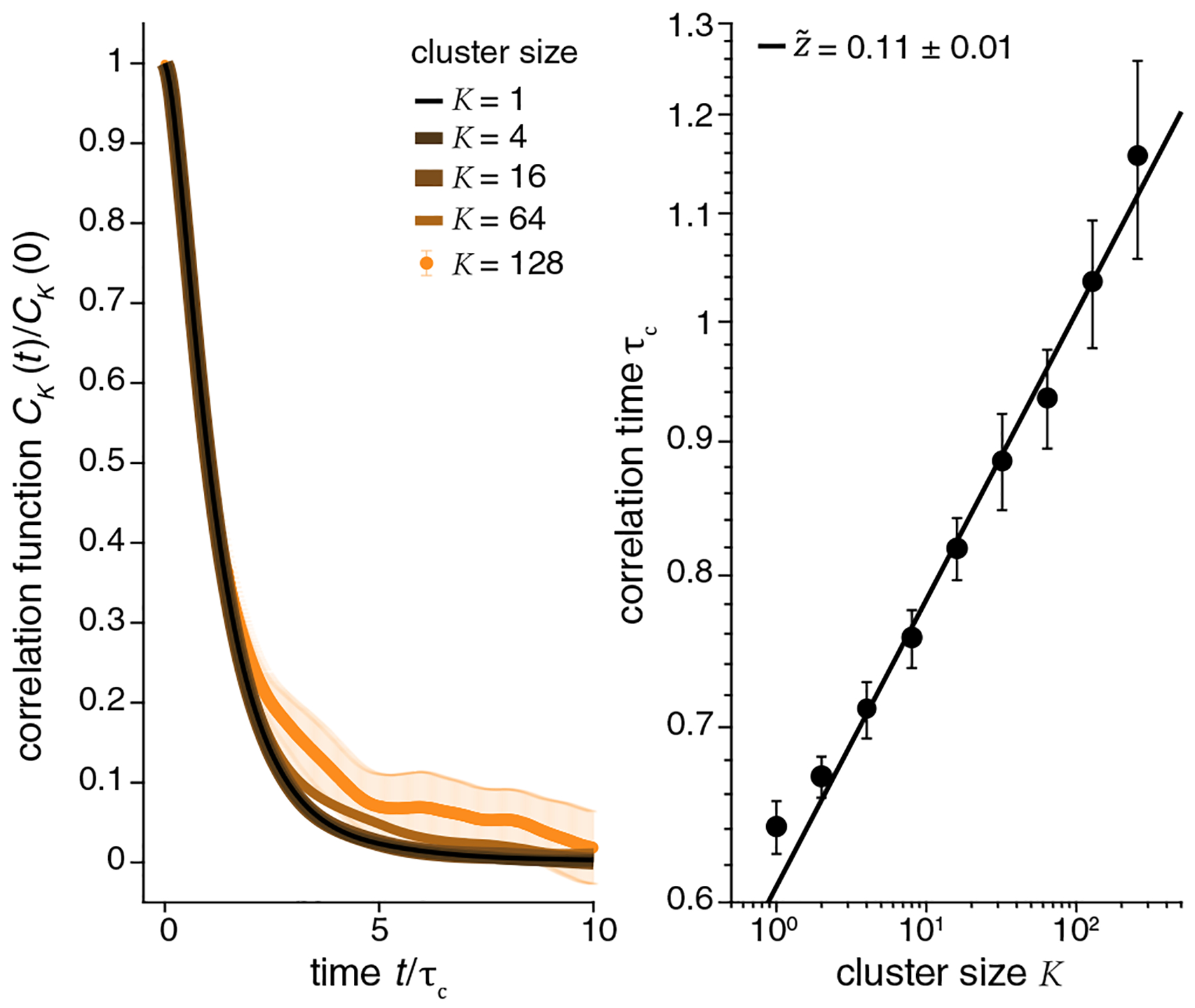
Dynamic scaling. (left) Correlation functions for different cluster sizes [Eq. (7)]. We show K = 1, 4, 16, 64, 128 (last one with error bars), where color lightens as K increases, illustrating the scaling behavior when we measure time in units of τ_c(K). (right) Dependence of correlation time on cluster size, with fit to Eq. (8).

Before interpreting these results, we make several observations, explored in detail elsewhere [23]. First, and most importantly, we have done the same experiment and analysis independently in three different mice; importantly there are no “identified neurons” in the mammalian brain, so we can revisit the same region of the hippocampus in another animal, but there is no sense in which we revisit the same neurons. Nonetheless we see the same approach to a fixed distribution and power-law scaling, with exponents measured in different animals having the same values within error bars; this is true even for $\tilde{\beta }$, which has error bars in the second decimal place. These results suggest, strongly, that behaviors we have identified are independent of variations in microscopic detail, as we hope.

Second, all the steps of analysis that we have followed here can be redone by discretizing the continuous fluorescence signals into binary on-off states for each neuron, as in Ref. [24]. Again we see an approach to a fixed non-Gaussian distribution, and power-law scaling; all exponents agree within error bars.

Third, we consider the relation of our observations to the salient qualitative fact about the rodent hippocampus, namely that many of the neurons in this brain area are “place cells.” These cells are active only when the animal visits a small, compact region of space, and silent otherwise; activity in the place cell population is thought to form a cognitive map that guides navigation [25,26]. This spatial localization of activity is preserved by our coarse-graining procedure, although it was not designed specifically to do this. In fact fewer than half of the cells in the population that we study are place cells in this particular environment, but after several steps of coarse-graining essentially all of the coarse-grained variables have well developed place fields. On the other hand, the scaling behavior that we see is not a simple consequence of place field structure. To test this, we estimate for each cell the probability of being active at each position, and then simulate a population of cells that are active with this probability but independently of one another; activity is driven by the observed trajectory of the mouse along the virtual track, and to compare with the fluorescence data we smooth the activity with a kernel matched to the known dynamics of the indicator molecule. In smaller populations this independent place cell model fails to capture important aspects of the correlation structure [24], and here we find that it does not exhibit the scaling shown in Figs. 3–5. These behaviors also do not arise in surrogate data sets that break the correlations among neurons.

Finally, we consider more generic model networks. We have simulated networks with continuous activity variables (“rate networks”) and random connections [27], as well as networks of spiking neurons in the asynchronous-irregular regime [28] that can generate some signatures of critical behavior without fine tuning [29]. In none of these simulations do we see scaling or the emergence of fixed non-Gaussian distributions of the coarse-grained variables; more details will be given elsewhere. The absence of scaling in these simulated networks confirms the intuition from statistical physics that arriving at a fixed point of the RG, with associated scaling behaviors, is not an accident. We conclude that our observations are not artifacts of limited data, are not generic features of neural networks, and are not simple consequences of known features of the neural response in this particular network.

In equilibrium statistical mechanics problems with local interactions, a fixed distribution and power-law scaling behaviors are signatures of a system poised near a critical point in its phase diagram. The idea that networks of neurons might be near to criticality has been discussed for more than a decade [30]. One version of this idea focuses on “avalanches” of sequential activity in neurons [31,32], by analogy to what happens in the early sandpile models for self-organized criticality [33]. In the human brain, it has been suggested that the large scale patterns of physical connectivity may be scale free or self-similar, providing a basis for self-similarity in neural activity [34,35]. A different version of the idea focuses on the distribution over microscopic states in the network at a single instant of time [36,37], and is more closely connected to criticality in equilibrium statistical mechanics. Related ideas have been explored in other biological systems, from biochemical and genetic networks [38–41] to flocks and swarms [42,43]. In our modern view, invariance of probability distributions under iterated coarse graining—a fixed point of the renormalization group—may be the most fundamental test for criticality, and has meaning independent of analogies to thermodynamics.

A fundamental result of the RG is the existence of irrelevant operators, which means that successive steps of coarse graining lead to simpler and more universal models. Although the RG transformation begins by reducing the number of degrees of freedom in the system, simplification does not result from this dimensionality reduction but rather from the flow through the space of models. The fact that our phenomenological approach to coarse-graining gives results that are familiar from successful applications of the RG in statistical physics encourages us to think that simpler and more universal theories of neural network dynamics are possible.

References

- [1].Kadanoff LP, Physics 2, 263 (1966). [Google Scholar]
- [2].Wilson KG, Rev. Mod. Phys 47, 773 (1975). [Google Scholar]
- [3].Wilson KG, Sci. Am 241, 158 (1979). [Google Scholar]
- [4].Cardy J, Scaling and Renormalization in Statistical Physics (Cambridge University Press, Cambridge, England, 1996). [Google Scholar]
- [5].Segev R, Goodhouse J, Puchalla JL, and Berry II MJ, Nat. Neurosci 7, 1155 (2004). [DOI] [PubMed] [Google Scholar]
- [6].Litke AM et al. , IEEE Trans. Nucl. Sci 51, 1434 (2004). [Google Scholar]
- [7].Harvey CD, Collman F, Dombeck DA, and Tank DW, Nature (London) 461, 941 (2009). [DOI] [PMC free article] [PubMed] [Google Scholar]
- [8].Marre O, Amodei D, Deshmukh N, Sadeghi K, Soo F, Holy TE, and Berry MJ, J. Neurosci 32, 14859 (2012). [DOI] [PMC free article] [PubMed] [Google Scholar]
- [9].Jun JJ et al. , Nature (London) 551, 232 (2017).29120427 [Google Scholar]
- [10].Chung JE, Joo HR, Fan JL, Liu DF, Barnett AH, Chen S, Geaghan-Breiner C, Karlsson MP, Karlsson M, Lee KY, Liang H, Magland JF, Pebbles JA, Tooker AC, Greengard L, Tolosa VM, and Frank LM, Neuron, 101, 21 (2019). [DOI] [PMC free article] [PubMed] [Google Scholar]
- [11].Dombeck DA, Harvey CD, Tian L, Looger LL, and Tank DW, Nat. Neurosci 13, 1433 (2010). [DOI] [PMC free article] [PubMed] [Google Scholar]
- [12].Harvey CD, Coen P, and Tank DW, Nature (London) 484, 62 (2012). [DOI] [PMC free article] [PubMed] [Google Scholar]
- [13].Ziv Y, Burns LD, Cocker ED, Hamel EO, Ghosh KK, Kitch LJ, El Gamal A, and Schnitzer MJ, Nat. Neurosci 16, 264 (2013). [DOI] [PMC free article] [PubMed] [Google Scholar]
- [14].Nguyen JP, Shipley FB, Linder AN, Plummer GS, Liu M, Setru SU, Shaevitz JW, and Leifer AM, Proc. Natl. Acad. Sci. U.S.A 113, E1074 (2016). [DOI] [PMC free article] [PubMed] [Google Scholar]
- [15].Gauthier JL and Tank DW, Neuron 99, 179 (2018). [DOI] [PMC free article] [PubMed] [Google Scholar]
- [16].Since we are using the strongest correlations, our coarse-graining procedure is not very sensitive to the spurious correlations that arise from finite sample size.
- [17].As an example, we could assign each neuron coordinates ri in a D dimensional space such that the correlations cij [Eq. (1)] are a (nearly) monotonic function of the distance dij = |ri − rj|; this is multidimensional scaling: J. B. Kruskal, Psychometrika 29, 1 (1964). As pointed out to us by MO Magnasco, our coarse-graining procedure then starts as local averaging in this abstract space, and it would be interesting to take this embedding seriously as way of recovering locality of the RG transformation. Other alternatives include using a more global, self-consistent definition of maximally correlated pairs, or using delayed correlations. More generally we can think of coarse graining as data compression, and we could use different metrics to define what is preserved in this compression.
- [18].When we use the renormalization group to study models, we indeed follow the flow of the joint distribution in various approximations [2,4]. When we are trying to analyze data, either from experiments or from simulations, this is not possible.
- [19].Binder K, Phys Z. B 43, 119 (1981). [Google Scholar]
- [20].Error bars for all scaling behaviors reported in this Letter were estimated as the standard deviation across quarters of the data. To respect temporal correlations, the location of the quarter was chosen at random, but time points remained in order inside it. For each quarter of the data, exponents are estimated as the slope of the best fit line on a log-log scale. We have also verified that there is no systematic dependence of our results on sample size.
- [21].Scaling usually is an asymptotic behavior, but, in Fig. 3, we see a power law across almost the full range from K = 1 to K = 512. If we fit only for K ≥ 32, for example, we find the same value of , within error bars; there is no sign that these larger values of K are more consistent with , Thanks to D. S. Fisher for asking about this.
- [22].For a discussion of the relation between RG and the spectra of covariance matrices, see; Bradde S and Bialek W, J. Stat. Phys 167, 462 (2017). [DOI] [PMC free article] [PubMed] [Google Scholar]
- [23].Meshulam L et al. , arXiv:1812. 11904. [Google Scholar]
- [24].Meshulam L, Gauthier JL, Brody CD, Tank DW, and Bialek W, Neuron 96, 1178 (2017). [DOI] [PMC free article] [PubMed] [Google Scholar]
- [25].O’Keefe J and Dostrovsky J, Brain Res. 34, 171 (1971). [DOI] [PubMed] [Google Scholar]
- [26].O’Keefe J and Nadel L, The Hippocampus as a Cognitive Map (Oxford, Clarendon Press, 1978). [Google Scholar]
- [27].Vogels TP, Rajan K, and Abbott LF, Annu. Rev. Neurosci 28, 357 (2005). [DOI] [PubMed] [Google Scholar]
- [28].Brunel NJ, J. Comp. Neurol 8, 183 (2000). [Google Scholar]
- [29].Touboul J and Destexhe A, Phys. Rev. E 95, 012413 (2017). [DOI] [PubMed] [Google Scholar]
- [30].Mora T and Bialek W, J. Stat. Phys 144, 268 (2011). [Google Scholar]
- [31].Beggs JM and Plenz D, J. Neurosci 23, 11167 (2003). [DOI] [PMC free article] [PubMed] [Google Scholar]
- [32].Friedman N, Ito S, Brinkman BAW, Shimono M, Lee DeVille RE, Dahmen KA, Beggs JM, and Butler TC, Phys. Rev. Lett 108, 208102 (2012). [DOI] [PubMed] [Google Scholar]
- [33].Bak P, Tang C, and Wiesenfeld K, Phys. Rev. Lett 59, 381 (1987). [DOI] [PubMed] [Google Scholar]
- [34].Zheng M et al. , arXiv:1904. 11793. [Google Scholar]
- [35].Betzel RF and Bassett DS, NeuroImage 160, 73 (2017). [DOI] [PMC free article] [PubMed] [Google Scholar]
- [36].Tkačik G, Schneidman E, Berry II MJ, and Bialek W, arXiv:q-bio/0611072. [Google Scholar]
- [37].Tkačik G, Mora T, Marre O, Amodei D, Palmer SE, Berry MJ, and Bialek W, Proc. Natl. Acad. Sci. U.S.A 112, 11508 (2015). [DOI] [PMC free article] [PubMed] [Google Scholar]
- [38].Socolar JES and Kauffman SA, Phys. Rev. Lett 90, 068702 (2003). [DOI] [PubMed] [Google Scholar]
- [39].Ramo P, Kesseli J, and Yli-Harja O, J. Theor. Biol 242, 164 (2006). [DOI] [PubMed] [Google Scholar]
- [40].Nykter M, Price ND, Aldana M, Ramsey SA, Kauffman SA, Hood LE, Yli-Harja O, and Shmulevich I, Proc. Natl. Acad. Sci. U.S.A 105, 1897 (2008). [DOI] [PMC free article] [PubMed] [Google Scholar]
- [41].Krotov D, Dubuis JO, Gregor T, and Bialek W, Proc. Natl. Acad. Sci. U.S.A 111, 3683 (2014). [DOI] [PMC free article] [PubMed] [Google Scholar]
- [42].Bialek W, Cavagna A, Giardina I, Mora T, Pohl O, Silvestri E, Viale M, and Walczak AM, Proc. Natl. Acad. Sci. U.S.A 111, 7212 (2014). [DOI] [PMC free article] [PubMed] [Google Scholar]
- [43].Cavagna A, Conti D, Creato C, Del Castello L, Giardina I, Grigera TS, Melillo S, Parisi L, and Viale M, Nat. Phys 13, 914 (2017). [Google Scholar]