Axonal actin in action: Imaging actin dynamics in neurons

Abstract

Actin is a highly conserved, key cytoskeletal protein involved in numerous structural and functional roles. In neurons, actin has been intensively investigated in axon terminals—growth cones—and dendritic spines, but details about actin structure and dynamics in axon shafts have remained obscure for decades. A major barrier in the field has been imaging actin. Actin exists as soluble monomers (G-actin) as well as actin filaments (F-actin), and labeling actin with conventional fluorescent probes like GFP/RFP typically leads to a diffuse haze that makes it difficult to discern kinetic behaviors. In a recent publication, we used F-actin selective probes to visualize actin dynamics in axons, resolving striking actin behaviors that have not been described before. However, using these probes to visualize actin dynamics is challenging as they can cause bundling of actin filaments; thus, experimental parameters need to be strictly optimized. Here we describe some practical methodological details related to using these probes for visualizing F-actin dynamics in axons.

INTRODUCTION

Actin is the most abundant protein in eukaryotic cells—an integral component of the cytoskeleton involved in cell motility, division, and signaling. In neurons, actin plays critical roles in axonal elongation, signaling, and synaptic homeostasis. The vast majority of studies on neuronal actin have focused on growth cones where actin is enriched, and many aspects of actin at this locale—such as retrograde flow—are well established (Dent, Merriam, & Hu, 2011; Letourneau, 2009). In cultured hippocampal neurons fixed/stained with fluorescent-phalloidin and visualized by light microscopy, actin at growth cones is readily visible due to its enrichment at this locale, but definite accumulations of F-actin are also seen along the axon shaft. Previous studies in large squid axons have also demonstrated subplasmalemmal as well as deep actin filaments (Bearer & Reese, 1999; Fath & Lasek, 1988), but the precise architecture and dynamics of actin in axons has been mysterious for decades.

Recent studies using superresolution microscopy in cultured hippocampal neurons revealed a dramatic picture of actin, with subplasmalemmal, circumferential actin rings wrapping underneath the plasma membrane (Xu, Zhong, & Zhuang, 2013). In a recent publication, we visualized the microanatomy and dynamics of F-actin using superresolution microscopy and live imaging, discovering an intricate, dynamic intra-axonal deep F-actin network that has not been characterized before (Ganguly et al., 2015). Here we describe additional practical details of the protocols we used for live imaging of F-actin in Ganguly et al. (2015). One of the challenges in live imaging of axonal actin is that actin exists as both monomers and polymers (F-actin) that are in a dynamic equilibrium. As about half of the actin in most cells is monomeric at any given time, tagging actin with conventional GFP/RFP fluoro-phores typically leads to a diffuse signal that obscures filament dynamics. Thus most studies in neurons using conventional probes have been limited to thin cytoplasmic extensions such as growth cones, and not thicker regions such as axonal shafts. Fortunately, recently developed selective F-actin binding probes such as Lifeact and Utr-CH (the calponin homology domain of actin-binding protein utrophin) (Burkel, von Dassow, & Bement, 2007; Riedl et al., 2008) circumvent this issue.

Here we will describe our own experience using F-actin binding probes in neurons. We have published detailed protocols on culturing hippocampal neurons and live imaging of axonal transport in these neurons (Ganguly & Roy, 2014; Roy, Yang, Tang, & Scott, 2011), and we will not repeat all those details. The purpose of this short article is mainly to serve as a practical guide for the experimentalist, and we expect that the methods described below will be used in conjunction with our published protocols of F-actin imaging (Ganguly et al., 2015) and general tips on live imaging (Ganguly & Roy, 2014; Roy et al., 2011). The most important point to consider when using either F-actin probe is to carefully titrate its expression levels so that F-actin dynamics are not perturbed. Below we will describe in detail techniques we have optimized in the lab to image F-actin in neurons with minimal or no apparent perturbation of actin dynamics.

Two F-actin binding probes have been commonly used to resolve F-actin behaviors: Lifeact and Utr-CH. Lifeact is a 17-amino-acid peptide from the yeast actin-binding protein 140 which binds to F-actin, though it also binds G-actin (Riedl et al., 2008). Since it has a lower binding affinity for F-actin than Utr-CH, it is thought to interfere less with actin dynamics. However, we find that moderate-to-high overexpression of Lifeact in neurons is equally problematic, and moreover its signal-to-noise ratio is lower than Utr-CH—limiting utility in precisely visualizing F-actin kinetics (see below). Utr-CH is based on the calponin homology domain of utrophin, an established F-actin binding protein in humans. With two actin binding sites, its high affinity binding faithfully reports F-actin, and it does not bind to G-actin (Burkel et al., 2007). While known technical limitations with the Utr-CH probe arise from its tendency to bundle actin filaments at high expression levels (Schuh, 2011), these limitations can be avoided by carefully controlling the expression of this probe. In this chapter we describe detailed methods that were used in our recent publication to visualize actin dynamics with both probes, with an emphasis on Utr-CH (Ganguly et al., 2015).

To study actin in axons, we transfected cultured hippocampal neurons with low levels of fluorescently tagged Utr-CH or Lifeact. But before collecting images, we applied rigorous selection criteria to exclude neurons overexpressing the F-actin probes at higher levels and avoid potential disruptions of actin dynamics. We also applied strict morphological criteria to ensure consistent axon selection, as we routinely do with all of our axonal transport studies. Time-lapse images of axonal actin dynamics were collected using a microscope system equipped with a highly sensitive EMCCD camera and capable of imaging two fluorophores with near-simultaneous time resolution.

1. MICROSCOPE SETUP FOR LIVE IMAGING

1.1. GENERAL INFORMATION

We performed live imaging on a Nikon Ti inverted fluorescence microscope equipped with a 40x and 100x oil-immersion objectives, a Lumencor Spectra LED light illuminator, and a QuantEM:512SC EMCCD camera (Photometrics). We routinely use 40x to identify transfected neurons and the 100x to perform live imaging. The microscope is equipped with a heated stage chamber set to ~ 37 °C (model STEV, World Precision Instrument, Inc. FL). The general optical setup is shown in Figure 1.

FIGURE 1. Setup for near-simultaneous dual-color imaging.

Rapid red (gray in print versions)/green (light gray in print versions) switching of excitation wavelengths with an LED, combined with sensitive detectors, allows rapid imaging of axonal kinetics in two channels (see text).

1.2. NEAR-SIMULTANEOUS DUAL-CHANNEL IMAGING

This setup allows for near-simultaneous dual-channel imaging of axonal dynamics, as shown in Figure 1. This is done by rapid (microsecond) switching of the red/green LEDs combined with a single multiband-pass filter (Chroma) and capturing images using a highly sensitive EMCCD camera. Two major challenges in dual-channel imaging of fast axonal dynamics with sufficient spatial and temporal resolution are acquisition speed and sensitivity of detection. Though the switching of fluoro-phores by LEDs is rapid, it is also critical that high-resolution images are captured in each channel, to allow clear detection of the fast dynamics. We found that using the EMCCD camera was important in this dual-channel imaging setup, as the exquisite sensitivity of the camera allowed us to keep exposure times (and thus time intervals between subsequent images) low, allowing us to capture the fast transport kinetics. This system allowed us to visualize F-actin dynamics and vesicle dynamics in the same axon; and for specific examples of dual-channel imaging, please see Ganguly et al. (2015). Below we focus on imaging F-actin dynamics.

2. PREPARATION OF NEURONS FOR IMAGING

2.1. NEURONAL CULTURE

Hippocampal cultures were obtained from brains of postnatal (P0–P1) CD-1 mice, and all protocols were followed in accordance with the University of California guidelines. The neurons were plated on MatTek glass bottom dishes at a density of 25,000 cells/10 mm dish. Once a week, the dishes were supplemented with 500 mL heated, fresh NB/B27 supplemented media. For a detailed protocol, see Ganguly and Roy (2014).

2.2. TRANSFECTION OF NEURONS

Neurons were cotransfected with the F-actin probe and a soluble RFP marker (see below) at 7–9 days in vitro (DIV) using Lipofectamine 2000 (Invitrogen). By DIV 7 the neurons are highly polarized, with thin elongated axons that are morphologically distinct from the broad, tapering dendrites. Typically, only a few neurons are transfected in each coverslip, which is ideal for these experiments. Transfection efficiency in our cultures starts dropping off around DIV 10. Transfection parameters needed to be strictly optimized for GFP:Utr-CH. To ensure low expression levels, neurons were transfected with one-fourth the amount of DNA routinely used in our laboratory—0.3 μg versus 1.2 μg DNA in 5 ml neurobasal/opti-MEM mixture used with Lipofectamine transfections. For a more detailed transfection protocol, see Ganguly and Roy (2014). Live imaging of axons was performed between 16 and 22 h after transfection with fluorescently tagged Utr-CH or Lifeact.

Axons are identified by their morphology (see Section 3.1 below for details), and it is important to cotransfect neurons with a spectrally distinct soluble volume filler that would help identify processes. Since the GFP:Utr-CH (or Lifeact) expression in these neurons is extremely dim, it is not practical to use these markers for identifying axons. Toward this we cotransfect neurons with soluble mRFP or mCherry, which is bright and spectrally distinct, allowing easy identification of dendrites and axons.

3. IMAGING AXONAL ACTIN

3.1. NEURONAL MORPHOLOGY AND AXON SELECTION

Healthy hippocampal neurons in culture grow in a predictable pattern (Kaech & Banker, 2006). As the neurons grow, several processes emerge from the neuronal soma; one of which becomes the axon and the others become dendrites. We prefer to grow neurons at a relatively high density (~ 2500 cells/mm), as they robustly differentiate into axons and dendrites (with established spines) and form functional synapses (Scott et al., 2010; Wang et al., 2014), allowing us to study neurons in a physiologic context. However such high-density cultures also make live imaging of axons challenging as axons and dendrites overlap, creating a complicated network. Low transfection efficiencies (using Lipofectamine) help as neurons are only sporadically labeled within the network. However, we have noticed that even with these methods, neurons often get transfected in clusters, with overlapping fluorescent axons and/or dendrites. Thus we have developed some standardized protocols in our laboratory to overcome these issues, allowing robust visualizing of dynamic processes in axons or dendrites (Das et al., 2013; Tang et al., 2012). These simple procedures lead to consistent, reliable data sets that allow comparisons between experimental conditions.

An example of the type of data set that can be obtained using consistent parameters is shown in Figure 2(A), where synaptophysin:mRFP-labeled vesicles were imaged in cultured hippocampal axons (adapted from one of our previous publications Tang et al., 2012). Each data-point in this graph represents the velocity of one particle in a given axon (y axis represents axon #1, axon #2, etc.). Note that though vesicles in a given axon move with a range of velocities, this range is fairly consistent from axon to axon and that overall anterograde velocities are consistently a bit faster than retrograde (see Tang et al., 2012 for more details). The key points for imaging F-actin in axons are detailed below.

FIGURE 2. Axon selection and other parameters for consideration in live imaging.

(A) Distribution of raw synaptophysin:mRFP transport data points in 25 axons, shown as an example of data that can be obtained with consistent imaging parameters. Note that though there is an intrinsic variability in the instantaneous velocities of particles moving within a given axon (mean ± standard deviation for each axon is also shown), the overall range of velocities is similar across multiple axons. Also note the slightly higher anterograde velocities (figure adapted from Tang et al. (2012), with permission). (B) A healthy neuron ideal for live imaging of the axon. The dendrites are marked by double arrowheads and the axon is marked by white arrowheads. A zoomed-in image of its dendrites and axons is shown on the right. Note the branched dendrites and a long, straight axon. (C) Examples of neurons that we typically avoid for live imaging of axonal kinetics. From top left to bottom right, the reasons for exclusion are the following: the origin of the axon is unclear; the axon branches too early; the axonal morphology is complicated and out of focus; the neuron appears to have two axons; axons from two neighboring transfected neurons appear to merge; and the axon is overlapping with another transfected process (processes of interest are marked by arrowheads, see text for details). All scale bars are 20 μm.

We typically use a soluble marker to define the morphology of neurons (typically untagged mRFP/mCherry, cotransfected with the GFP-tagged protein of interest), and apply rigorous selection criteria for choosing axons for live imaging. Neurons are scanned at 40x to select an axon, and thereafter all dynamic imaging is done at 100x magnification. Only neurons with unambiguous morphology, where axons can be confidently identified are selected for imaging. Using these criteria (see below), only a small subset of neurons in any given coverslip can be imaged (typically <10, out of 20–30 transfected neurons). Though labor-intensive, we found that these data-collection procedures are important for obtaining consistent and meaningful data sets in experiments using F-actin probes.

In general, axons are identifiable by their long, thin processes that typically branch at ~90° angles, unlike thicker dendrites that are tapering and branch at more acute angles. For consistency, we also image axon segments that are within 150 μM of the soma, but well-distal to the axon initiation segment (which is within the first 20–40 μM in these neurons). Our inclusion/exclusion criteria for selecting optimal neurons/axons are described below with examples (Figure 2(B) and (C)). Specific criteria are as follows:

• 1.The dendrites are well branched and the axon is easily distinguished.
• 2.The axon segment selected for imaging is relatively straight and lies in the focal plane of imaging (the latter can usually only be definitely determined at 100x magnification).
• 3.The axon does not branch in the first 150 μM where the F-actin will be imaged. This is an important but often neglected technical aspect of axonal live imaging, as physical laws dictate that branching of axons proximal to the region imaged will decrease the frequency of cargoes that are exported from the soma. We think that his might be the reason for low transport rates seen in some studies where only distal thin axons (easy to image) are examined.

An example of an optimal neuron is shown in Figure 2(B). Note that there are several dendrites that branch at acute angles (double arrowheads). The axon emerging from the soma (white arrowheads) is relatively straight and unbranched for the first ~ 200 μm, and the axon eventually branches, giving rise to a long, thin process transecting the right half of the image. Figure 2(C) shows several examples of neurons that we avoid in such studies. Shown in the top left panel of Figure 2(C) is a neuron with an axon whose origin cannot be determined confidently. Near the soma, it can be difficult to identify the beginning of the axon in the midst of the dendritic arbor. If the point where the axon originates is not immediately clear, we try to find a branch of the axon which has grown past the dendritic arbor (the longest processes are axonal) and then try tracing the axon back to the soma by following the various axon branch-points (which are usually easy to identify). If the point of origin still cannot be identified, there is no way to ensure that the axon is imaged at a consistent distance from the soma and we avoid these neurons. The top middle panel of Figure 2(C) shows a neuron with an easily distinguishable axon emerging from the soma. However, the axon branches soon after the axon initial segment and therefore does not meet our imaging criteria. In the top right panel of Figure 2(C), a straight, easily identifiable axon can be seen. But even at 40x, it is clear that the morphology of this axon is complicated, and only parts of the axon lie in the focal plane of the image, making imaging anything more than a few micrometer segment impossible at 100x.

In the bottom left panel of Figure 2(C), the neuron shown appears to have two axons. In these cases, usually the second axon belongs to a neighboring transfected neuron; but if there is any ambiguity in identification, we do not use the neuron for live imaging. In the bottom middle panel of Figure 2(C) are two neighboring neurons that have been transfected, and it is sometimes difficult to assign the right axon to the right neuron. As mentioned above we see this frequently with Lipofectamine transfections, and while it is sometimes possible to distinguish between the axons of two neighboring transfected neurons, it is often just better to move on to another neuron in the coverslip that has unambiguous morphology. Finally, the bottom right panel of Figure 2(C) shows a transfected axon overlapping with another dendritic process. It is important not to image the overlapping segment, as dynamics in the nearby process would be indistinguishable from movement in the axon of interest.

3.2. CHARACTERIZATION OF ACTIN PROBES

Though these F-actin probes have been extensively characterized in the literature, their use in neurons has been limited. To characterize these probes in neurons, we transfected cells with GFP:Utr-CH or Lifeact:GFP, and then fixed and stained them with rhodamine-tagged phalloidin (F-actin marker). Neurons were fixed with 4% paraformaldehyde dissolved in a cytoskeletal preservation buffer (10 mM MES, pH 6.1, 150 mM NaCl, 5 mM EGTA, 5 mM glucose, and 5 mM MgCl₂; see Ganguly et al., 2015). As shown in Figure 3(A) and (B), Utr-CH and Lifeact distribution is identical to the phalloidin staining. Also note that the phalloidin staining in transfected neurons is identical to that in untransfected ones (Figure 3(C)), providing further confidence that under our specific experimental conditions, the tools used to visualize F-actin are not bundling actin.

FIGURE 3. Fidelity of F-actin reporters in neurons.

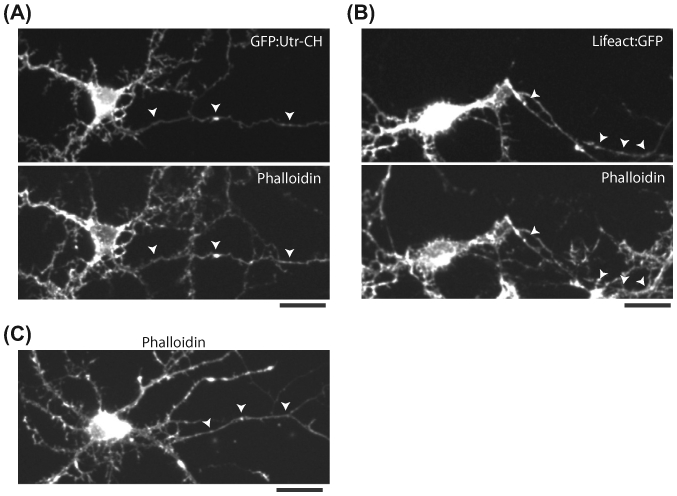
(A) Neuron transfected with GFP:Utr-CH (top panel) and fixed and stained with rhodamine-phalloidin (bottom panel, axon marked by arrowheads). Note an almost complete overlap of GFP:Utr-CH and F-actin in the transfected neuron. (B) Neuron transfected with Lifeact:GFP (top panel) and fixed and stained with rhodamine-phalloidin (bottom panel, axon marked by arrowheads). Note an almost complete overlap of Lifeact:GFP and F-actin in the transfected neuron. All scale bars are 20 μm. (C) Rhodamine-phalloidin staining of an untransfected neuron. Note punctate F-actin accumulations along the axon (marked by arrowheads). Also note accumulations in dendritic shafts and spines.

3.3. SELECTION OF LOW EXPRESSERS

We found that high overexpression of both Utr-CH and Lifeact in neurons lead to nonphysiologic bundling of F-actin, also reported by other studies in nonneuronal cells (Schuh, 2011). Thus we developed strict criteria for selecting/imaging Utr-CH/Lifeact transfected neurons, to avoid imaging overexpressers. Below we describe our criteria for selecting low expressers of GFP:Utr-CH:

• 1.Discrete bright patches of F-actin in the soma (likely corresponding to F-actin localizing at the Golgi).
• 2.No F-actin “cables/spikes” in the soma/dendrites (see below and Figure 4).
• 3.A faint, speckled appearance of F-actin within the dendritic shafts.
• 4.F-actin puncta along the axon with minimal diffuse fluorescence.

FIGURE 4. Examples of low and high GFP:Utr-CH expressers.

(A) Somatodendritic (top) and corresponding axonal (bottom) regions of three neurons with low levels of GFP:Utr-CH expression, suitable for imaging axonal F-actin dynamics. Note patchy accumulations of F-actin in the soma (dashed ellipse), probably representing F-actin at the Golgi. Insets show scaled regions of interest, highlighting GFP:Utr-CH fluorescence within axon shafts (see text). Also note the strikingly punctate fluorescence in axons, with essentially no background fluorescence (lower panels, puncta in axons marked by arrowheads). (B) Somatodendritic (top) and corresponding axonal (bottom) images showing moderate GFP:Utr-CH overexpressers, not suitable for imaging axonal F-actin dynamics. In general, numerous spiky cables of F-actin are seen in the soma and proximal dendrites, somatic patches of F-actin are not clearly visible, and there is a diffuse fluorescence in axons with large F-actin accumulations. Note that though actin patches in the soma are seen in the neuron on the left, its axon (below) has abnormal F-actin accumulation. (C) An obvious high GFP:Utr-CH overexpresser with extensive spiky F-actin cables in the soma/dendrites and abnormal accumulations of F-actin in axons. All images were independently scaled to maximize bit-depth and highlight specific features as detailed above. Scale bars are 20 μm.

Even when transfecting low amounts of DNA for the probes, we see that only ~25% of the transfected neurons meet these criteria. Figure 4(A) shows three examples of low expressers that do meet the criteria described above. In contrast to the low expressers shown in Figure 4(A), neurons overexpressing higher levels of GFP:Utr-CH are shown in Figure 4(B) and (C). In general, we identified gradients of overexpression patterns, and though the very high expressers were quite obvious, it was important to also identify the ones that expressed somewhat lower levels but also had nonphysiologic distribution of F-actin (see below) and did not show much F-actin kinetics upon live imaging. Our criteria for excluding moderate-to-high overexpressers—all of which showed absent or limited F-actin dynamics—are described below.

The left panel of Figure 4(B) shows a neuron that just crosses our threshold for high overexpression. Note that while there are patches of F-actin in the soma, they are confluent and numerous. Importantly, the F-actin distribution along the axon of this neuron (bottom panel) is continuous, unlike the punctate distribution seen in lower expressers (the numerous axonal filopodia are also probably a result of overexpression). The middle and right panels in Figure 4(B) show examples of neurons that are more obviously overexpressing GFP:Utr-CH at high levels. Note that there is significant bundling of F-actin in the soma/dendrites, leading to “cables” or “spikes” of F-actin. Also note the diffuse F-actin fluorescence in axons (panels below), with large accumulations. Figure 4(C) shows an example of a neuron that is expressing very high levels of GFP:Utr-CH. Note numerous “F-actin bundles” in this neuron, leading to large “cables/spikes” of F-actin in the cell body and dendritic shafts. Also note the abnormal clumping of F-actin in the axon.

In our cultured neurons, the overexpression patterns of GFP:Utr-CH and GFP: Lifeact appear similar, so we apply the same selection process to find low expressers in either case. However, we have empirically noticed that Lifeact does not cause the pronounced bundling of F-actin that is sometimes seen with GFP:Utr-CH (as in Figure 4(C)), likely due to the lower affinity of Lifeact for F-actin. However as mentioned above, signal-to-noise ratio was lower for Lifeact, and we feel that when used carefully, GFP:Utr-CH is an excellent probe for reporting F-actin behaviors.

3.4. PARAMETERS FOR LIVE IMAGING OF AXONAL ACTIN DYNAMICS

The steps we use to image actin in the axon are detailed below. Our neurons typically grow in a Neurobasal/B27-based media, in a CO2 incubator at 37 °C, and have to be transferred into a Hibernate-E-based media for live imaging. These methods have been described in detail in our previous publications (Ganguly & Roy, 2014; Roy et al., 2011) and are summarized here. Below we assume that the neuron has been cotransfected with GFP:Utr-CH and soluble mCherry.

• 1.Warm up “live imaging media” (Hibernate-E medium, 2 mM GlutaMAX, 0.4% D-Glucose, 37.5 mM NaCl, 2% B27) to 37 °C in a water bath (see Ganguly & Roy, 2014 for detailed instructions on making “live imaging media”).
• 2.Warm up the heated stage chamber to 37 °C.
• 3.Remove the Neurobasal/B27 media from the dish to be imaged, wash twice with 1 mL of “live imaging media,” and then add 1 mL of warm media to the dish for live imaging.
• 4.Place the dish in the heated stage chamber and wait for 10 min, allowing the temperature of the dish, the oil, and the surface of the objective to equilibrate. We find that this minimizes disruptions to the focal plane from temperature fluctuations.
• 5.Switch to the 40x objective/GFP filters and scan the neurons transfected with GFP: Utr-CH. Select a low expresser based on the criteria described in Section 3.3.
• 6.After identifying a low expresser, switch to the RFP channel and view the soluble RFP/mCherry marker. Make sure that the neuron meets the morphological criteria described in Section 3.1. If not, find another low expresser and try again. The goal here is to identify the proximal axon of a low GFP:Utr-CH expresser as noted above. It is also important to note down the direction of the axon at this point.
• 7.After identifying a suitable axon, switch to the 100x objective and, from this point on, view the axon with the live-feed from the camera (this mimics imaging conditions). At 100x magnification, check again that there is a straight, unbranched segment of the axon 50—150 μm from the soma that lies in one focal plane. Note that the entirety of the axon 50—150 μm from the soma does not need to be in focus, simply the short segment that one needs to image at 100x (typically ~ 40—50 μm).
• 8.Constrict the field diaphragm in the light path of the microscope so that only the axonal segment to be imaged live is exposed to light. This will prevent pho-tobleaching of GFP:Utr-CH outside the area of imaging.
• 9.Switch to the GFP channel and start imaging.

We typically image F-actin probes at a rate of one frame per second, and each movie lasts 600 s. For our microscope setup, 400 ms exposure with 20% intensity LED GFP/RFP light is ideal to both detect the F-actin dynamics and minimize photobleaching. The same parameters are also used for near-simultaneous dualchannel imaging. Actin dynamics are usually seen by the first minute of imaging. After capturing a video, a kymograph of the F-actin movement in the axon is created using standard procedures (drop-down menus in Metamorph or Nikon Elements software). Representative kymographs from low expressers of GFP:Utr-CH and Lifeact:GFP are shown in Figure 5(A). Note the diagonal plumes of fluorescence representing rapid polymerization of actin (“actin trails,” a few marked by arrowheads) and “hotspots” of actin along the axon, represented by vertical interrupted lines in our kymographs. Also note that though the overall kinetics of Utr-CH and Lifeact are very similar (see Ganguly et al., 2015 for quantification of both), a diffuse fluorescence is seen with Lifeact, likely because it also binds to G-actin, and the signal-to-noise ratio is generally lower. Figure 5(B) shows exemplary axonal kymographs from neurons that are overexpressing GFP:Utr-CH and Lifeact:GFP at high levels. Note that F-actin kinetics are absent in these axons. Finally, Figure 6 shows kymographs from near-simultaneous dual-imaging of GFP:Utr-CH and Life-act:mCherry in the same axon. Note some common actin kinetics in both kymographs, marked by arrowheads.

FIGURE 5. Exemplary kymographs from F-actin imaging in axons.

(A) Representative kymographs from neurons expressing either GFP:Utr-CH or Lifeact:GFP at low levels. Time in seconds is shown on left/right. Note diagonal plumes of fluorescence representing actin polymerization in axons (“actin trails,” a few marked by arrowheads), as well as “hotspots” along the axon where actin appears to polymerize/depolymerize (vertical lines in the kymographs). Also note the diffuse haze in the Lifeact:GFP kymographs, probably due to G-actin binding. (B) Kymographs from neurons expressing high levels of GFP:Utr-CH or Lifeact:GFP. Note that the dynamic F-actin behaviors described above (actin trails and hotspots) are not apparent when the neuron is overexpressing the F-actin binding probes.

FIGURE 6. Near-simultaneous dual-channel imaging of GFP:Utr-CH and Lifeact:mCherry.

Neurons were cotransfected with low levels of GFP:Utr-CH and Lifeact:mCherry, and axons were selected using the criteria described in the text. Kymographs from GFP (left) and RFP (right) channels of one such experiment are shown. Note the correspondence of F-actin kinetics detected by these two probes (a few common events marked by arrowheads) though the signal-to-noise ratio from Lifeact is lower as mentioned in the text.

Imaging actin has been a challenge in the field for a long time, and selective F-actin binding probes have revealed a dramatic new world of actin in many different cell types. However these probes also induce polymerization of actin, and careful experimental design and data interpretation is critical. For reasons that are unclear at this time, neurons seem particularly sensitive to high overexpression of both Utr-CH and Lifeact—compared to other cell types where these probes have been extensively used—and we hope that the above experiential observations will be useful to the community.

REFERENCES

- Bearer EL, & Reese TS (1999). Association of actin filaments with axonal microtubule tracts. Journal of Neurocytology, 28, 85–98. [DOI] [PMC free article] [PubMed] [Google Scholar]
- Burkel BM, von Dassow G, & Bement WM (2007). Versatile fluorescent probes for actin filaments based on the actin-binding domain of utrophin. Cell Motility and the Cyto-skeleton, 64, 822–832. [DOI] [PMC free article] [PubMed] [Google Scholar]
- Das U, Scott DA, Ganguly A, Koo EH, Tang Y, & Roy S (2013). Activity-induced convergence of APP and BACE-1 in acidic microdomains via an endocytosis-dependent pathway. Neuron, 79, 447–460. [DOI] [PMC free article] [PubMed] [Google Scholar]
- Dent EW, Merriam EB, & Hu X (2011). The dynamic cytoskeleton: backbone of den-dritic spine plasticity. Current Opinion in Neurobiology, 21, 175–181. [DOI] [PMC free article] [PubMed] [Google Scholar]
- Fath KR, & Lasek RJ (1988). Two classes of actin microfilaments are associated with the inner cytoskeleton of axons. Journal of Cell Biology, 107, 613–621. [DOI] [PMC free article] [PubMed] [Google Scholar]
- Ganguly A, & Roy S (2014). Using photoactivatable GFP to track axonal transport kinetics. Methods in Molecular Biology, 1148, 203–215. [DOI] [PubMed] [Google Scholar]
- Ganguly A, Tang Y, Wang L, Ladt K, Loi J, Dargent B, et al. (2015). A dynamic for-min-dependent deep F-actin network in axons. Journal of Cell Biology, 210(3). 10.1083/jcb.201506110. [DOI] [PMC free article] [PubMed] [Google Scholar]
- Kaech S, & Banker G (2006). Culturing hippocampal neurons. Nature Protocols, 1, 2406–2415. [DOI] [PubMed] [Google Scholar]
- Letourneau PC (2009). Actin in axons: stable scaffolds and dynamic filaments. Results and Problems in Cell Differentiation, 48, 65–90. [DOI] [PubMed] [Google Scholar]
- Riedl J, Crevenna AH, Kessenbrock K, Yu JH, Neukirchen D, Bista M, et al. (2008). Lifeact: a versatile marker to visualize F-actin. Nature Methods, 5, 605–607. [DOI] [PMC free article] [PubMed] [Google Scholar]
- Roy S, Yang G, Tang Y, & Scott DA (2011). A simple photoactivation and image analysis module for visualizing and analyzing axonal transport with high temporal resolution. Nature Protocols, 7, 62–68. [DOI] [PMC free article] [PubMed] [Google Scholar]
- Schuh M (2011). An actin-dependent mechanism for long-range vesicle transport. Nature Cell Biology, 13, 1431–1436. [DOI] [PMC free article] [PubMed] [Google Scholar]
- Scott DA, Tabarean I, Tang Y, Cartier A, Masliah E, & Roy S (2010). A pathologic cascade leading to synaptic dysfunction in alpha-synuclein-induced neurodegeneration. Journal of Neuroscience, 30, 8083–8095. [DOI] [PMC free article] [PubMed] [Google Scholar]
- Tang Y, Scott DA, Das U, Edland SD, Radomski K, Koo EH, et al. (2012). Early and selective impairments in axonal transport kinetics of synaptic cargoes induced by soluble amyloid beta-protein oligomers. Traffic, 13, 681–693. [DOI] [PMC free article] [PubMed] [Google Scholar]
- Wang L, Das U, Scott DA, Tang Y, McLean PJ, & Roy S (2014). Alpha-synuclein multimers cluster synaptic vesicles and attenuate recycling. Current Biology, 24, 2319–2326. [DOI] [PMC free article] [PubMed] [Google Scholar]
- Xu K, Zhong G, & Zhuang X (2013). Actin, spectrin, and associated proteins form a periodic cytoskeletal structure in axons. Science, 339, 452–456. [DOI] [PMC free article] [PubMed] [Google Scholar]