Reliable cross-docking location problem under the risk of disruptions

Abstract

This paper seeks to develop a reliable network of cross-docks by taking in to account disruption and reliability issues to hedge against heterogeneous risk of cross-docking failure. In real environments, applying a recovery policy can be a feasible strategy to handle disruptions. Hence, in this study, a recovery policy has been addressed in the form of reallocating suppliers to alternative cross-docks or altering the transportation strategy to move shipments. In addition to cross-dock location design, the optimum capacity of opened cross-docks will be determined considering the loads that will be served by each cross-docking center under regular and disruption conditions. A mixed integer nonlinear programming formulation is presented for the problem and is then linearized to present an efficient model. In order to solve it, two Lagrangian relaxation algorithms are designed and tested on 40 problem instances with different values of parameters. The results achieved by GAMS/CPLEX are compared with those of two algorithms and some analyses are performed on the solutions. Moreover, as the case study, the focus has been placed on logistic part of a car-manufacturing company with a vast supply chain network, containing more than 600 suppliers. The logistic strategies have been applied in order to reduce the transportation cost through the supply chain network and diminish the disruption subsequences in such a network. Based on the results, some managerial recommendations are presented.

Introduction

In classical facility location problems, all facilities are assumed reliable and optimal facility locations are determined in this ideal environment. However, in practice, the facilities face numerous unexpected events that may partially or completely disable them (Xie et al. 2015). A consequence of these facility failures may be a higher transportation cost since customers need to be reassigned from their initial facilities to another operational facility that is more distant (Snyder and Daskin 2005; Cui et al. 2010; Berman et al. 2007). Therefore, designing a reliable supply chain network is one of the most effective approaches to deal with disruption risks, failures and uncertainties since alternative plans in the event of a disruption are mostly limited.

Generally, uncertainties and risks in the supply chains can be classified into two major categories including operational risks and disruptions. Risks at operational levels are short term and daily problems that mostly do not affect the functionality of the elements of supply chains. Some examples of operational risks are machine failures, short-term supply–demand imbalances, procurement prices for raw materials, production costs, poor process performance, decrease in production rate of a machine, lead times or transportation times (Ahmadi-Javid and Seddighi 2013). However, disruptions can completely or partly block the flow of products in the network for a significant and uncertain amount of time. Disruptions can be caused by natural disasters (e.g. earthquakes, floods, and hurricanes), terrorist attacks, labor strikes, political instability, power outages, sabotage or even equipment breakdowns. Some events such as the Severe Acute Respiratory Syndrome (SARS) outbreak in Asia, the September 11, 2001 terrorist attack, the hurricanes Katrina and Rita (2005), and more recent disasters like earthquake and Tsunami in Japan, 2011, highlighted the necessity to protect supply chains against disruption (Berman et al. 2009).

Disruption management strategies can be categorized into three main classes: mitigation strategies (in advance of a disruption), recovery strategies (after the occurrence of a disruption), and passive acceptance (Paul et al. 2016). Some examples of mitigation strategies are increasing the safety stock, multiple sourcing, increasing capacity, etc. Recovery strategies consist of using alternative sourcing, rescheduling of plans and rerouting the transportation plan in recovery periods. In this study, we deal with a recovery strategy, in which once a disruption happens, the alternative plan will be applied to hedge against it. Considered network consists of suppliers, cross-docks (as consolidation points) and assembly plants which are connected to suppliers via two transportation methods: cross-docking and direct shipment.

Cross-docking helps to accelerate the flow of parts and material, reduces the number of vehicles and diminishes inventory costs. The main purpose of cross-docking in almost all companies is to collect various supply products in the form of pallets (boxes), consolidate them into a collection of mixed pallets of products with the same destination, and dropped them off at the consume point (manufacturing/assembly plants/end user), according to the orders. Cross-docking can reduce cost in distribution networks by consolidation, as well as applying full-truck-load (FTL) shipments, instead of delivering all shipments directly and in less-than-truck-load (LTL). Note that incoming pallets are usually delivered to the cross-dock facility in LTL shipments, while outgoing pallets are shipped in FTL. The goal is to maximize the utilization of FTL shipments in order to decrease transportation and distribution cost. To function correctly, a reliable system of cross-docks and a precise coordination of inbound/outbound vehicles are essential (Ladier and Alpan 2016). In other words, cross-docking is an approach to implement just-in-time (JIT) strategy. Based on recent studies, JIT may make supply chains more vulnerable to local and global disturbances. It adds vulnerability in supply process when delays, failures, accidents, breakdowns, or fluctuation in demand occur (Ebrahimi et al. 2012).

As a real case, the earthquakes and tsunami in Japan 2011 reflected the vulnerability of companies to supply chain disruptions caused by natural disasters, and pinpointed the JIT strategy pioneered by Toyota and followed by many other companies. After the occurrence of such events, companies made efforts to address these problems by applying recovery plans, such as using alternative suppliers. Another recovery plan in the supply chains with distribution centers is using alternative distribution facilities in the case of disruption, in which, instead of considering many scenarios for disruption, a set of distribution centers are assigned to every supplier. Each supplier is served by the nearest distribution center and if disruption happens, it will get service from the second one in the set and so on. This approach can be utilized in food, clothing and auto making industries, etc.

In this study, we design a cross-docking network that is both reliable and cost efficient. It takes disruption risk in to consideration, which seems that has not been addressed, so far, in cross-docking. Based on cross-docking literature, uncertainty is mostly handled by robust optimization technique and fuzzy approach in cross-docking, while in this study, the aim is to generate recovery plans to manage disruptions at cross-docks after occurrence, without enumerating all possible failure scenarios. In a scenario-based method, a large number of probabilistic failure scenarios may complicate the problem (Zhang et al. 2016) and increase the computational effort.

Here, therefore, the optimal location of a set of cross-docking centers is decided, when cross-docks are subject to disruption. To do so, a location model is developed to minimize establishing cost of cross-docks, transportation costs in both regular and failure conditions and penalty cost of not serving suppliers and plants. By solving the model, the optimal number and locations of cross-docking centers, as well as the initial and back up assignments of suppliers and assembly plants to cross-docks are determined. Moreover, regarding regular and disruption conditions, the optimal capacity of cross-docks can be specified using the formulation, which is another extension to previous reliability models. The model is formulated as a mixed integer nonlinear programming model, then it is linearized to present a linear model and finally two Lagrangian relaxation methods are proposed as solution algorithms.

The remainder of this study is organized as follows. Section 2 presents a relevant literature review. In Sect. 3, the problem and mathematical model with heterogeneous disruption probabilities are introduced and linearization process is explained. Lagrangian relaxation methods as the solution algorithms are presented in Sect. 4 and computational tests along with numerical results are addressed in Sect. 5. In this section, a case study is investigated, as well. Finally, we conclude the study in Sect. 6.

Literature

Because of inherent stochastic nature of cross-docking, considering disruption in such environment is unavoidable, while it has not drawn much attention in the literature. Some papers address uncertainty in location problem of cross-docking, as well as in other design or implementation levels, while some others considered a deterministic environment for various cross-docking problems.

Location problem in cross-docking can be seen in Sung and Song (2003), Gumus and Bookbinder (2004), Jayaraman and Ross (2003), Ross and Jayaraman (2008), Bachlaus et al. (2008), Musa et al. (2010), Mousavi and Tavakkoli-Moghaddam (2013), and Mousavi et al. (2014). In these studies, the best location of cross-docks is determined without considering the risk of disruptions. Very few research works tackle uncertainties on the operational level. Babazadeh et al. (2014) propose a robust optimization model for location problem in a responsive supply chain consisting of plants, warehouses and cross-docks. They first presented a multi-stage multi-product deterministic mixed-integer linear programming (MILP) model and then addressed the robust optimization to handle the uncertainty of parameters. Ladier and Alpan (2016) also use robust optimization for handling uncertainties in truck scheduling in which delay of trucks is the source of uncertainty. They apply classical techniques of robust optimization (minimax and minimization of the expected regret) and techniques from robust project scheduling (resource redundancy and time redundancy) to the problem. Afterward, Rahbari et al (2019) utilized two robust models in order to consider the uncertainty of travel time and freshness-life of perishable products in vehicle routing problem with cross-docking (VRPCD). In a paper by Darvishi et al. (2020), the tactical planning level is focused. The authors apply an approach based on hybrid fuzzy-robust stochastic method in production planning with cross-docking.

So far, no research work has addressed disruption in cross-docking strategy, to the best of our knowledge. Hence, a brief review on reliable location problems is presented, in which the location of general facilities is determined.

The reliable facility location problem was probably first introduced by Snyder and Daskin (2005) to handle facility disruption, where the authors assume that some facilities are subject to random failure with equal probability, while the others are reliable. In their problem, excessive transportation costs may be burden because of serving customers by more distant facilities compared to their regularly assigned ones. They develop a bi-objective linear integer programming model based on level assignments, where the first objective represents the total travel cost to initial facilities in regular condition (the first level assignment) and the second objective indicates the expected transportation cost after facility failures. The authors apply a Lagrangian relaxation solution method to solve the model. Another study that develops this approach is the work of Berman et al. (2007), which is based on the P-median problem. They relax the assumption of identical failure probabilities and formulated the stochastic problem as a nonlinear mixed integer program. They also prove that the solution to the stochastic P-median problem with zero failure probabilities is equal to the solution of deterministic problem. The authors develop several exact and heuristic methods to the problem. Based on their work, Cui et al. (2010) and Shen et al. (2011) also relax the equal failure probability assumption in Snyder and Daskin (2005) and allow the failure probabilities to be facility-specific and independent (the probabilities are taken as a priori). Cui et al. (2010) propose a mixed-integer programming formulation and a continuum approximation model to optimize the initial establishment cost and the expected transportation costs under regular and disruption conditions. Both papers consider R ≥ 1 level to assignment of customers, which means that each customer can be assigned to R facilities. The authors provide several heuristic solution algorithms. Shen et al. (2011) also study a similar reliable facility location problem and formulate it as a two-stage stochastic nonlinear integer programming (NIP) model. They propose an approximation algorithm for a special case where the failure probability of a facility is independent of the facility. In their study, the uncertainty is modeled via two approaches: (1) by a set of scenarios that determines which subset of facilities are subject to a failure and (2) by considering an individual and independent failure probability for each facility. They also provide several heuristics for the problem.

In the study of Berman et al. (2009), the location of facilities is addressed in an environment that customers are not aware in advance about whether a given facility is operational or not, therefore they may go to several facilities to find an operational one. Seeking for automated teller machines (ATMs) is an example, where a customer may have to try several ATMs before finding one able to provide service, due to network disruptions, maintenance, etc. The authors present a model that try to locate a set of facilities to minimize the total expected cost of customer travel including travel, reliability and information costs. Lim et al. (2010) also apply a similar approach to manage disruption in location problem. They define two classes of facilities: reliable (which are not subject to failure, but are more expensive) and unreliable and formulate the problem as a mixed integer programming (MIP) model. A Lagrangian relaxation-based algorithm is developed as a solution method.

Some extensions of reliable location problem can be found in the literature. Chen et al. (2011) integrated inventory and reliable facility location problems. Li and Ouyang (2010) address a problem in which facilities are subject to heterogeneous and spatially correlated disruptions and Li et al. (2013b) further propose a supporting station model to manage interdependent facility disruptions. In Li et al. (2013b), a new model is proposed to transform correlated and complex facility failures (e.g., those due to common disasters) into independent and identically distributed (i.i.d.) disruptions in a supporting structure framework. They generate a mathematical model for reliable facility location problem under correlated facility disruption, which is formulated into a compact integer linear program and can be efficiently solved by usual solvers.

Li et al. (2013a) develop a reliable P-median problem and a reliable un-capacitated fixed-charge location problem, where the facility failure probabilities are assumed to be independent and location-specific. They also consider one layer of supplier backup and facility fortification with a limited budget. A Lagrangian relaxation-based (LR) method is developed to solve the models. Jalali et al. (2016) study a bi-objective reliable facility location problem for a three-echelon supply chain network. In their model, provider-side uncertainty is also considered. As the proposed model is NP-hard, the authors use an algorithm called multi-objective biogeography-based optimization (MOBBO) and compare the results with non-dominated ranking genetic algorithm (NRGA) and a multi-objective simulated annealing (MOSA). Another related model is proposed in Zarrinpoor et al. (2017) that address reliable location model for design of health service network. The authors formulate the problem based on robust optimization approach and solve it using Benders decomposition algorithm. Other similar works can be seen in Zhang et al. (2016), Rohaninejad et al. (2018), Jabbarzadeh et al. (2018), Raziei et al. (2018), Esfandiyari et al. (2018), Torkestani et al. (2018), Bashiri et al. (2018); and finally, Yahyaei and Bozorgi-Amiri (2018). Many other researchers are inspired by this method of handling disruption and even utilized it in location routing problem (see Zhang et al. 2015).

Although several studies consider disruption in supply chain networks (Kleindorfer and Saad 2009; Schmitt 2011; Zegordi and Davarzani 2012; Qiang and Nagurney 2012; Qi 2013; Hishamuddin et al. 2013, 2014; Shi et al. 2013; Kim et al. 2014; Bode and Wagner 2015; Zhao et al. 2019), there are not considerable studies addressing disruption in cross-docking.

In this paper, we focus on a cross-dock location model, where cross-docks may be subject to disruptions, causing suppliers and assembly plants to seek service from other operating cross-docks or use direct shipment strategy. Despite a wide range of publications in reliable facility location problem, very few considered reliable cross-docking problem. For example, Hasani Goodarzi et al. (2018) address disruption in cross-docking, when disruption probabilities are the same for all cross-docking center, which is a simplifying assumption.

In most studies reviewed in reliable facility location, the authors suppose that certain facilities are designated as indefectible, though in this paper we assume all cross-docks as unreliable and direct shipment as a safe way to move consignments. The probabilities of cross-dock failure are assumed to be heterogeneous, since identical failure probability is reasonable in the case of similar facilities, such as ATMs.

The problem we seek to formulate is how to optimally locate a set of |J| cross-docking centers on a network when cross-docks are subject to disruption, without enumerating all possible failure scenarios. Drawing inspiration from literature, we develop a reliable location problem for cross-docking network, where all built cross-docks are subject to independent and cross-dock specific disruption probability. The model allocates suppliers and plants to cross-docks at multiple levels. The “higher-level” allocations are only realized when the primary cross-docks are subject to a disruption. As can be inferred from literature, disruption issues have not been addressed perfectly in cross-docking so far and it seems that robust optimization is a common method to address uncertainty in cross-docking. In other words, there is no piece of research considering disruption in cross-docking, to the best of authors’ knowledge. Therefore, in this study, the aim is to generate recovery plans to manage disruptions at cross-docks after occurrence. Another extension to previous works is that optimal capacity of cross-docks is specified regarding regular and disruption conditions using the formulation.

Problem definition

This study addresses a network in which cross-docks are considered as consolidation nodes serving the suppliers and assembly plants. We assume that when a cross-dock is disrupted, one can use other cross-docking centers as backups instead of building a new one, until the regular operating conditions are re-established. In addition to cross-docking strategy, it is also possible to use direct shipment whenever it is economic. Each supplier and assembly plant can be assigned to up to |R| ≥ 1 cross-docks. Although each supplier will be served by only one operational cross-dock, it needs to be assigned to a group of cross-docks that are ordered by levels, meaning that when the lowest-level facility is subject to a failure, the service is provided by the next level cross-dock that is operational; and so on. Another backup plan can be direct shipment strategy which means that if all operational cross-docks are too far away from a supplier, direct shipment can be utilized.

In order elaborate the concept of level in this problem, let us give an example. Consider 10 suppliers, 3 cross-docks and 2 assembly plants. In the first level (r = 1), the normal condition is considered and the assignment of suppliers to cross-docks is as bellow, which means that cross-dock 1 serves supplier 4 and 9, cross-dock 2 serves supplier 5, 7 and 8; and cross-dock 3 serves supplier 1, 2, 3 and 10. Supplier 6 sends all products through direct shipment (see Table 1).

Table 1.

Assignment of suppliers to cross-docks at level 1

Supplier	1	2	3	4	5	6	7	8	9	10
Cross-dock	3	3	3	1	2	-	2	2	1	3

Now the goal is to define a backup strategy (including cross-docking or direct shipment) for each supplier, independent of other suppliers. It must be different from the previous assigned cross-dock (see Table 2). The second level assignment (r = 2) meaning that if a cross-dock fails, its assigned suppliers are allocated to other cross-docks or to direct shipment. For example, both suppliers 1 and 10, at normal condition, are allocated to cross-dock 3, but if a disruption happens to this cross-dock, the first supplier is assigned to cross-dock 2, while suppler 10 is served by direct shipment.

Table 2.

Assignment of suppliers to cross-docks at level 2

Supplier	1	2	3	4	5	6	7	8	9	10
Cross-dock	2	1	1	3	3	-	3	1	–	–

In order to compare scenario-based method with this approach, consider this problem in a scenario-based format. There are eleven different scenarios for failure in cross-docks: (1) all cross-docks are normal (1 case), (2) all cross-docks are disrupted (1 case), (3) one of cross-docks is disrupted (6 cases), (4) two of cross-dock are disrupted (3 cases). As can be inferred, “a large number of probabilistic failure scenarios complicates the problem” (Zhang et al. 2016) and increases the computational effort. While in our approach, every cross-dock is considered, separately.

It should be noted that using direct shipment is possible at each level, if it is less costly compared to cross-docking, meaning that the same cardinality |R| of the support is assumed for all suppliers, while all or some of them may be assigned to direct shipment in level r <|R|. If direct shipment is assigned to a supplier in a given level, he/she cannot be served by a cross-dock in the subsequent levels. Therefore, the cross-docking reliability problem extends the cross-docking location problem taking into account the random disruptions of cross-docks. Other assumptions are as follows:

• Cross-docking disruptions are independent and heterogeneous meaning that each cross-dock may fail with a given specific probability and multiple cross-docks may fail simultaneously. All cross-docks are considered unreliable and each may have a level of reliability.

• Backup plan can be decided in multi-levels (|R| ≥ 1). At each level, each supplier can be served at most by one cross-dock, while assembly plants can receive parts from more than one cross-dock.

• A penalty cost is considered for cases in which disruption causes a supplier not to be served at all (by any of the assigned cross-docking centers or direct shipment).

• As mentioned above, when a disruption occurs, it seems more reasonable to use other cross-docking centers or change the transportation strategy from cross-docking to direct shipment until the disruptive event is repaired. In the cases that disruption leads to the permanent destruction of one or more cross-docks, resolving the location problem will be recommended. In other words, when a huge disruption occurs in such a way that a cross-dock cannot be utilized any more, it is better to resolve a location problem to find a new point to establish an alternative cross-dock.

In Fig. 1, the supply chain network is indicated in a typical level. It is obvious that in various levels, the configuration of network is different. The problem addresses: (1) the location of cross-docks, (2) the initial allocation of suppliers and assembly plants to cross-docks and (3) back up plan for allocation in the case of disruption in cross-docking centers. Moreover, the best capacity of opened cross-docks, as well as the transportation strategy in each level to move parts from suppliers to assembly plants is determined. The objective is to minimize the total cross-dock establishing cost and the expected transportation and penalty costs.

Fig. 1.

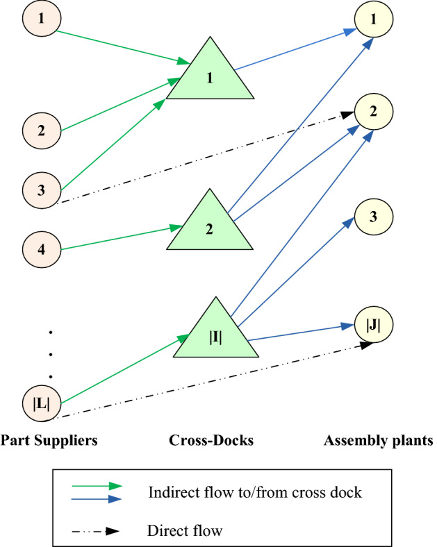
The supply chain network at a typical level

Mathematical model

In this sub-section, we first introduce the notation and the decision variables used throughout the study. We then formulate the problem as a mixed integer nonlinear programming model. The sets, parameters and variables used in the model are described in the following sub-section.

Sets and parameters

Define J to be the set of assembly plants {j = 1, 2, …, |J|}, I to be the set of candidate cross-docks {i = 1, 2, …, |I|}, L to be the set of suppliers {l = 1, 2, …, |L|}and finally, R as the set of levels {r = 1, …, |R|}. The term “Node” will be used to represent the assembly plants, suppliers and cross-docks. We assume that probability of failure in each cross-dock is given by $0\le q_i<1$, and cross-dock disruptions are independent of each other. When a cross-dock fails, it cannot provide service and its assigned nodes will be either served by other operational facilities, or linked by direct shipment. In the cases that no transportation strategy is used, it will be subject to a penalty cost. According to our assumptions, each supplier is assigned to up to R cross-docks (1 ≤ R ≤ |I| + 1) and can be served only by these cross-docks. The demand of plant j from supplier l is denoted by d_jl that must be met by vehicles with capacity Q. Transportation cost from node i to node j (i, j ∈ (L ∪ I ∪ J)) is given by c_ij. Parameter g_i represents the fixed cost of establishing cross-dock i and v_i is the variable cost per part unit at this cross-dock. Associated with each supplier l is a cost ${\gamma }_l$ that represents the penalty cost for not serving that supplier. The parameters are briefly listed as follows:

c_ij

Transportation cost from node i to node j (i, j ∈(L∪I∪J))

g_i

Fixed cost of establishing cross-dock i

v_i

Variable cost per part unit at cross-dock i

q_i

Probability of failure in cross-dock i ($0\le q_i<1$)

d_jl

Demand of plant j from supplier l

Q

Capacity of vehicles

${\gamma }_l$

Penalty for not serving supplier l

Decision variables

U_ljr

1: if load from supplier l to plant j is sent directly at level r; 0: otherwise

y_i

1: if cross-dock i is open; 0: otherwise

Z_ilr

1: if load from supplier l is served by cross-dock i at level r; 0: otherwise

m_lir

The number of vehicles from supplier l to cross-dock i at level r

n_ijr

The number of vehicles from cross-dock i to plant j at level r

B_lijr

1: if demand of plant j from supplier l goes thorough cross-dock i at level r; 0: otherwise

w_ijr

Quantity of parts shipped from cross-dock i to plant j at level r

P_lir

Probability that cross-dock i serves supplier l at level r

PP_lr

Probability that direct shipment serves supplier l at level r

Pr_ijr

Probability that cross-dock i serves plant j at level r

${\beta }_l$

Probability that supplier l will not be served at all

Cap_i

Capacity of cross-dock i.

Mathematical formulation

With the notations introduced above, the problem can be formulated as a mathematical model (CDL-NLP) as follows:

$$\begin{array}{cc}& \left(\text{CDL}-\text{NLP}\right)\hfill \\ \hfill & Min\sum _{i\in I}{g}_i\times y_i+\sum _{r\in R}\sum _{j\in J}\sum _{l\in L}{c}_{\mathit{lj}}\times P{P}_{\mathit{lr}}\times U_{\mathit{ljr}}+\sum _{r\in R}\sum _{i\in I}\sum _{l\in L}{c}_{\mathit{li}}\times m_{\mathit{lir}}\times P_{\mathit{lir}}\hfill \\ \hfill & +\sum _{r\in R}\sum _{i\in I}\sum _{l\in L}\sum _{j\in J}{v}_i\times d_{\mathit{jl}}\times B_{\mathit{lijr}}\times P_{\mathit{lir}}+\sum _{r\in R}\sum _{i\in I}\sum _{l\in L}{c}_{\mathit{ij}}\times n_{\mathit{ijr}}\times P{r}_{\mathit{ijr}}+\sum _{l\in L}^{}{\beta }_l\times {\gamma }_l\hfill \\ \hfill \end{array}$$ 1

$$\begin{array}{cc}& \text{Subject}\text{to}\hfill \\ \hfill & U_{\mathit{ljr}}+\sum _{i\in I}{B}_{\mathit{lijr}}=1;\forall l,j,r\hfill \\ \hfill \end{array}$$ 2

$$\sum _{r\in R}^{}{Z}_{\mathit{ilr}}\le y_i;\forall i,l$$ 3

$$\sum _{j\in I}{B}_{\mathit{lijr}}\times d_{\mathit{jl}}\le m_{\mathit{lir}}\times Q;\forall l,i,r$$ 4

$$\sum _{l\in L}{d}_{\mathit{jl}}\times B_{\mathit{lijr}}-w_{\mathit{ijr}}=0;\forall i,j,r$$ 5

$$Z_{\mathit{ilr}}\le \sum _{j\in J}{B}_{\mathit{lijr}};\forall l,i,r$$ 6

$$\sum _{j\in J}{B}_{\mathit{lijr}}\le \left|J\right|\times Z_{\mathit{ilr}};\forall l,i,r$$ 7

$$w_{\mathit{ijr}}\le n_{\mathit{ijr}}\times Q;\forall i,j,r$$ 8

$$P_{li1}=1-q_i;\forall l,i$$ 9

$$P_{\mathit{lir}}=\left(1-q_i\right)\times \sum _{k=1}^I\frac{q_k}{1-q_k}\times P_{lkr-1}\times Z_{klr-1};\forall l,i;2\le r\le \left|R\right|$$ 10

$$P{P}_{l1}=1;\forall l$$ 11

$$P{P}_{\mathit{lr}}=\sum _{k=1}^I\frac{q_k}{1-q_k}\times P_{lkr-1}\times Z_{klr-1};\forall l;2\le r\le \left|R\right|$$ 12

$$P{r}_{\mathit{ijr}}=\frac{{\sum }_l^{}{d}_{\mathit{jl}}\times B_{\mathit{lijr}}\times P_{\mathit{lir}}}{w_{\mathit{ijr}}+\epsilon };\forall i,j,r$$ 13

$${\beta }_l=\sum _{k=1}^I\frac{q_k}{1-q_k}\times P_{\mathit{lkR}}\times Z_{\mathit{klR}};\forall l$$ 14

$$Ca{p}_i=ma{x}_r\left(\sum _{j\in J}{w}_{\mathit{ijr}}\right);\forall i$$ 15

$$y_i,U_{\mathit{ljr}},B_{\mathit{lijr}},Z_{\mathit{ilr}}\in \left\{0,1\right\}$$ 16

$$m_{\mathit{lir}},n_{\mathit{ijr}},w_{\mathit{ijr}}\in \left\{0,1,2,\dots \right\}$$ 17

$$P_{\mathit{lir}},P{P}_{\mathit{lr}},P{r}_{\mathit{ijr}},{\beta }_l\in \left[0,1\right]$$ 18

The objective function minimizes the total expected cost including the fixed cost of establishing cross-docks, the expected transportation costs (including direct transshipment cost, indirect transportation cost from suppliers to cross-docks, variable cross-docking cost at receiving process and delivery cost to assembly plants) and finally the expected penalty cost. Constraint (2) ensures that demand of each plant is supplied via cross-docks or direct transshipment at each level. constraint (3) limits supplier assignments to only the open cross-docks, while constraint (4) stipulates the maximum vehicle capacity and calculates the number of required vehicles from suppliers to cross-docks at each level. Equation (5) determines the load to be sent from cross-docks to assembly plants and ensures that at each level, a flow entering a cross-dock is equal to the flow exiting it.

Constraints (6) and (7) ensure that when Σj B_lijr is positive, then Z_ilr should be equal to one, otherwise Z_ilr = 0. These constraints stipulate that cross-dock i gives service to supplier l, if B_lijr is equal to one, at least for one assembly plant. Constraint (8) determines the number of vehicles shipped from each cross-dock to each plant in different levels. Equations (9–13) are the “probability” equations. In Eqs. (9) and (10), the probability that a cross-dock serves a supplier at each level is determined recursively, while in Eqs. (11) and (12) the probability that direct shipment is used to serve suppliers at different levels is calculated. Based on Eqs. (9) and (10), the probability that a cross-dock serves a plant at each level is determined in Eq. (13). In order to avoid an undetermined value for this equation, we add a small value ($\epsilon$) in the denominator. Equation (14) finds the probability that a supplier is not served at all. Finally, constraint (15) determines the optimum capacity of each cross-dock. The types of decision variables are defined in (16–18).

The proposed formulation is a nonlinear model consisting of |I| + |L||R|(|J| + |I||J| + |I|) binary variables, (|L| + 2|J|) |R||I| integer variables, |R|(|I||L| + |L| + |I||J|) + |L| continues variables and |R|(|L||J| + 3|I||L| + 3|I||J|) + 2|L|(|I| + 1) + (|R| − 1)|L|(|I| + 1) active constraints. It can be reduced to un-capacitated facility location problem if (1) cross-docking is the only transportation strategy and no direct shipment is allowed (by increasing the cost of direct shipment to a very big number), (2) all cross-docks are perfectly reliable ($q_i=0\forall i\in \text{I}$), so all assignments are at the primary level (R = 1) and penalty cost is zero, thus the model is reducible to a two-level extension of classical facility location problem. The latter is known to be NP-hard as acclaimed by Nemhauser and Wolsey (1999); therefore, the studied problem is NP-hard as well.

Linearization

There are some nonlinear terms in the mathematical model and the solver is not able to find a solution in a reasonable time, even for small instances. As can be seen in the mathematical model (CDL-NLP), the objective function (1) and constraints (10), (12–14) are nonlinear. It should be noted that Eq. (15) could be simply calculated after running the model, while its linearization process is presented here, as well. In this section, we try to linearize the nonlinear terms and constraints. In order to do so, first the linearization of objective function is implemented. In the objective function (1), the following terms are nonlinear:

$$\sum _{r\in R}\sum _{j\in J}\sum _{l\in L}{c}_{\mathit{lj}}\times P{P}_{\mathit{lr}}\times U_{\mathit{ljr}}$$

$$\sum _{r\in R}\sum _{i\in I}\sum _{l\in L}{c}_{\mathit{li}}\times m_{\mathit{lir}}\times P_{\mathit{lir}}$$

$$\sum _{r\in R}\sum _{i\in I}\sum _{l\in L}\sum _{j\in J}{v}_i\times d_{\mathit{jl}}\times B_{\mathit{lijr}}\times P_{\mathit{lir}}$$

$$\sum _{r\in R}\sum _{i\in I}\sum _{l\in L}{c}_{\mathit{ij}}\times n_{\mathit{ijr}}\times P{r}_{\mathit{ijr}}$$

We define $P{P}_{\mathit{lr}}\times U_{\mathit{ljr}}$ as ${\mu }_{\mathit{ljr}}$, and $B_{\mathit{lijr}}\times P_{\mathit{lir}}$ as ${ϵ}_{\mathit{lijr}}$. The following Eqs. (19)−(26) demonstrate the linearization process of these two terms of objective function.

$$P{P}_{\mathit{lr}}\times U_{\mathit{ljr}}={\mu }_{\mathit{ljr}};\forall l,j,r$$

$${\mu }_{\mathit{ljr}}\le U_{\mathit{ljr}};\forall l,j,r$$ 19

$${\mu }_{\mathit{ljr}}\le P{P}_{\mathit{lr}};\forall l,j,r$$ 20

$$P{P}_{\mathit{lr}}\le {\mu }_{\mathit{ljr}}+\left(1-U_{\mathit{ljr}}\right);\forall l,j,r$$ 21

$${\mu }_{\mathit{ljr}}\ge 0;\forall l,j,r$$ 22

$$B_{\mathit{lijr}}\times P_{\mathit{lir}}={ϵ}_{\mathit{lijr}};\forall l,i,j,r$$

$${ϵ}_{\mathit{lijr}}\le B_{\mathit{lijr}};\forall l,i,j,r$$ 23

$${ϵ}_{\mathit{lijr}}\le P_{\mathit{lir}};\forall l,i,j,r$$ 24

$$P_{\mathit{lir}}\le {ϵ}_{\mathit{lijr}}+\left(1-B_{\mathit{lijr}}\right);\forall l,i,j,r$$ 25

$${ϵ}_{\mathit{lijr}}\ge 0;\forall l,i,j,r$$ 26

For $m_{\mathit{lir}}\times P_{\mathit{lir}}$, as well as $n_{\mathit{ijr}}\times P{r}_{\mathit{ijr}}$ linearization is not as straightforward as the above process, since in these cases the product of an integer and a continuous variable needs to be linearized. In order to do so, we show $m_{\mathit{lir}}$ and $n_{\mathit{ijr}}$ by m and n and define an upper bound equal to M and N for them, respectively. Then, we replace the integer variables of m and n by a series of binary variables $m_t^{\prime }$ and $n_j^{\prime }$, i.e. $m={\sum }_{t=0}^{M}t{m}_t^{\prime }=1m_1^{\prime }+2m_2^{\prime }+3m_3^{\prime }+\cdots +M{m}_M^{\prime }$ and $n={\sum }_{h=0}^{N}h{n}_h^{\prime }$ ($m_t^{\prime }$ and $n_h^{\prime }\in \left\{0,1\right\}$). Each product of integers now is a product of binaries and product of the corresponding binary variables can be linearized simply. Equations (27)−(32) and (33)−(38) show the linearization process for $m_{\mathit{lir}}\times P_{\mathit{lir}}$ and $n_{\mathit{ijr}}\times P{r}_{\mathit{ijr}}$, respectively.

$$m_{\mathit{lir}}\times P_{\mathit{lir}}={\varphi }_{\mathit{lir}};\forall l,i,r$$

$$m_{\mathit{lir}}=\sum _{t=0}^{M}t{m}_{\mathit{lirt}}^{\prime };\forall l,i,r$$ 27

$${\varphi }_{\mathit{lir}}=\sum _{t=0}^M{\varphi }_{\mathit{lirt}}^{\prime };\forall l,i,r$$ 28

$${\varphi }_{\mathit{lirt}}^{\prime }\le t{P}_{\mathit{lir}};\forall l,i,r,t$$ 29

$${\varphi }_{\mathit{lirt}}^{\prime }\le t{m}_{\mathit{lirt}}^{\prime };\forall l,i,r,t$$ 30

$${\varphi }_{\mathit{lirt}}^{\prime }\ge t{P}_{\mathit{lir}}+t\left(m_{\mathit{lirt}}^{\prime }-1\right);\forall l,i,r,t$$ 31

$$m_{\mathit{lirt}}^{\prime }\in \left\{0,1\right\};{\varphi }_{\mathit{lirt}}^{\prime }\ge 0;\forall l,i,r,t$$ 32

$$n_{\mathit{ijr}}\times P{r}_{\mathit{ijr}}={\mathrm{\pounds }}_{\mathit{ijr}};\forall i,j,r$$

$$n_{\mathit{ijr}}=\sum _{h=0}^{N}h{n}_{\mathit{ijrh}}^{\prime };\forall i,j,r$$ 33

$${\mathrm{\pounds }}_{\mathit{ijr}}=\sum _{h=0}^N{{\mathrm{\pounds }}^{\prime }}_{\mathit{ijrh}};\forall i,j,r$$ 34

$${{\mathrm{\pounds }}^{\prime }}_{\mathit{ijrh}}\le hP{r}_{\mathit{ijr}};\forall i,j,r,h$$ 35

$${{\mathrm{\pounds }}^{\prime }}_{\mathit{ijrh}}\le h{n}_{\mathit{ijrh}}^{\prime };\forall i,j,r,h$$ 36

$${{\mathrm{\pounds }}^{\prime }}_{\mathit{ijrh}}\ge hP{r}_{\mathit{ijr}}+h\left(n_{\mathit{ijrh}}^{\prime }-1\right);\forall i,j,r,h$$ 37

$$n_{\mathit{ijrh}}^{\prime }\in \left\{0,1\right\};{{\mathrm{\pounds }}^{\prime }}_{\mathit{ijrh}}\ge 0;\forall i,j,r,h$$ 38

Linearization of constraints (10), (12) and (14) is implemented using constraints (39)–(42). Although Eqs. (10), (12) and (14) are nonlinear, the only nonlinear term is $P_{\mathit{lkr}}\times Z_{\mathit{klr}}$, which is a product of a continuous and a binary variable. We replace each $P_{\mathit{lkr}}\times Z_{\mathit{klr}}$ with a new variable ${\theta }_{\mathit{klr}}$ and a set of new constraints (39)–(42) is added to the programming model.

$$P_{\mathit{lkr}}\times Z_{\mathit{klr}}={\theta }_{\mathit{klr}};\forall k,l,r$$

$${\theta }_{\mathit{klr}}\le Z_{\mathit{klr}};\forall k,l,r$$ 39

$${\theta }_{\mathit{klr}}\le P_{\mathit{lkr}};\forall k,l,r$$ 40

$$P_{\mathit{lkr}}\le {\theta }_{\mathit{klr}}+\left(1-Z_{\mathit{klr}}\right);\forall k,l,r$$ 41

$${\theta }_{\mathit{klr}}\ge 0;\forall k,l,r$$ 42

In constraint (13), some modifications are needed to linearize the equation. In this constraint, $P{r}_{\mathit{ijr}}$ and $w_{\mathit{ijr}}$ are continuous and integer variables, respectively. Therefore, in order to linearize this constraint, the method explained before (for two terms of objective function) will be applied again. This method is implemented in constraints (43)–(51).

$$P{r}_{\mathit{ijr}}=\frac{{\sum }_l^{}{d}_{\mathit{jl}}\times B_{\mathit{lijr}}\times P_{\mathit{lir}}}{w_{\mathit{ijr}}+\epsilon };\forall i,j,r$$

$$P{r}_{\mathit{ijr}}\left(w_{\mathit{ijr}}+\epsilon \right)=\sum _l^{}{d}_{\mathit{jl}}\times B_{\mathit{lijr}}\times P_{\mathit{lir}};\forall i,j,r$$ 43

$$P{r}_{\mathit{ijr}}\left(w_{\mathit{ijr}}+\epsilon \right)=\sum _l^{}{d}_{\mathit{jl}}\times {ϵ}_{\mathit{lijr}};\forall i,j,r$$ 44

$${\alpha }_{\mathit{ijr}}+\epsilon P{r}_{\mathit{ijr}}=\sum _l^{}{d}_{\mathit{jl}}\times {ϵ}_{\mathit{lijr}};\forall i,j,r$$ 45

$$w_{\mathit{ijr}}\times P{r}_{\mathit{ijr}}={\alpha }_{\mathit{ijr}};\forall i,j,r$$

$$w_{\mathit{ijr}}=\sum _{b=1}^{W}b{w}_{\mathit{ijrb}}^{\prime };\forall i,j,r$$ 46

$${\alpha }_{\mathit{ijr}}=\sum _{b=1}^W{\alpha }_{\mathit{ijrb}}^{\prime };\forall i,j,r$$ 47

$${\alpha }_{\mathit{ijrb}}^{\prime }\le bP{r}_{\mathit{ijr}};\forall i,j,r,b$$ 48

$${\alpha }_{\mathit{ijrb}}^{\prime }\le b{w}_{\mathit{ijrb}}^{\prime };\forall i,j,r,b$$ 49

$${\alpha }_{\mathit{ijrb}}^{\prime }\ge bP{r}_{\mathit{ijr}}+b(w_{\mathit{ijrb}}^{\prime }-1);\forall i,j,r,b$$ 50

$$w_{\mathit{ijrb}}^{\prime }\in \left\{0,1\right\};{\alpha }_{\mathit{ijrb}}^{\prime }\ge 0;\forall i,j,r,b$$ 51

In order to wte constraint (15) in a simpler linear fashion, first consider this new variable $W_{\mathit{ir}}$ as ${\sum }_{j\in J}{w}_{\mathit{ijr}};\forall i,r$. The linearization process is as follows.

$$Ca{p}_i=ma{x}_r\left(\sum _{j\in J}{w}_{\mathit{ijr}}\right);\forall i$$ 15

$$W_{\mathit{ir}}=\sum _{j\in J}{w}_{\mathit{ijr}};\forall i,r$$ 52

$$W_{\mathit{ir}}\le Ca{p}_i;\forall i,r$$ 53

$$W_{\mathit{ir}}\ge Ca{p}_i-\left(1-{\tau }_r\right)M;\forall i,r$$ 54

$$\sum _{r\in R}{\tau }_r\ge 1;$$ 55

$${\tau }_r\in \left\{0,1\right\};W_{\mathit{ir}}\ge 0$$ 56

Regarding the linearization of nonlinear constraints, the following model (CDL-LP) will be achieved:

$$\begin{array}{cc}& (\text{CDL}-\text{LP})\hfill \\ \hfill & Min\sum _{i\in I}{g}_i\times y_i+\sum _{r\in R}\sum _{j\in J}\sum _{l\in L}{c}_{\mathit{lj}}\times {\mu }_{\mathit{ljr}}+\sum _{r\in R}\sum _{i\in I}\sum _{l\in L}{c}_{\mathit{li}}\times {\varphi }_{\mathit{lir}}\hfill \\ \hfill & +\sum _{r\in R}\sum _{i\in I}\sum _{l\in L}\sum _{j\in J}{v}_i\times d_{\mathit{jl}}\times {ϵ}_{\mathit{lijr}}+\sum _{r\in R}\sum _{i\in I}\sum _{l\in L}{c}_{\mathit{ij}}\times {\mathrm{\pounds }}_{\mathit{ijr}}+\sum _{l\in L}^{}{\beta }_l\times {\gamma }_l\hfill \\ \hfill \end{array}$$ 57

$$\begin{array}{cc}& \text{Subject to}\hfill \\ \hfill & \left(2\right)-\left(9\right)\hfill \\ \hfill & \left(11\right)\hfill \\ \hfill & \left(16\right)-\left(18\right)\hfill \\ \hfill & \left(19\right)-\left(42\right)\hfill \\ \hfill & \left(45\right)-\left(56\right)\hfill \\ \hfill \end{array}$$

$$P_{\mathit{lir}}=\left(1-q_i\right)\times \sum _{k=1}^I\frac{q_k}{1-q_k}\times {\theta }_{klr-1};\forall l,i;2\le r\le \left|R\right|$$ 58

$$P{P}_{\mathit{lr}}=\sum _{k=1}^I\frac{q_k}{1-q_k}\times {\theta }_{klr-1};\forall l;2\le r\le \left|R\right|$$ 59

$${\beta }_l=\sum _{k=1}^I\frac{q_k}{1-q_k}\times {\theta }_{\mathit{klR}};\forall l$$ 60

Unlike most scenario-based stochastic programming formulations that have exponential number of variables and constraints, the proposed formulation is polynomial in size. In other words, it attempts to find the best solution without enumerating all possible combinatorial disruption scenarios. As indicated by Cui et al. (2010), if |R| = |I|, then the programming model is equal to stochastic programming formulation that covers all disruption scenarios. One can refer to Cui et al. (2010) for more details.

Programming formulation with identical disruption probability q

When the disruption probability is the same for all cross-docking centers, the original model (CDL-NLP) simply changes to cross-docking location problem with homogenous disruption probability (HDCDL). This problem has been introduced by Hasani Goodarzi et al. (2018) as a mixed integer linear programming model, whose model is presented in “Appendix 1”. Parameter q represents the identical failure probability for all cross-docks. In order to validate the proposed formulation (CDL-NLP), we compared it with model (HDCDL), where all q_i values are set to q in (CDL-NLP). A simple proof for this assertion is presented here. In the model (CDL-NLP), consider all $q_i$ values as q. Thus, constraint (10) changes to the following constraint.

$$P_{\mathit{lr}}=\left(1-q\right)\times \frac{q}{1-q}\times P_{lr-1}=q\times P_{lr-1}=q^2\times P_{lr-2}=q^{r-1}\times P_{l1}=q^{r-1}\left(1-q\right)$$ 61

Based on above equation, the probability of using direct shipment for suppliers in level r ($P{P}_{\mathit{lr}}$) is $q^{r-1}$. Constraint (13) of model (CDL-NLP), the probability of serving plant j by cross-dock i, is modified to the following constraint.

$$P{r}_{\mathit{jr}}=\frac{{\sum }_l^{}{d}_{\mathit{jl}}\times B_{\mathit{lijr}}\times P_{\mathit{lr}}}{w_{\mathit{ijr}}+0.0001}=\frac{q^{r-1}\left(1-q\right){\sum }_l^{}{d}_{\mathit{jl}}\times B_{\mathit{lijr}}}{w_{\mathit{ijr}}+\epsilon }=q^{r-1}\left(1-q\right);\forall i,j,r$$ 62

Finally, ${\beta }_l$ is calculated regarding this constraint:

$${\beta }_l=\frac{q}{1-q}\times P_{\mathit{lR}}=\frac{q}{1-q}\times q^{R-1}\left(1-q\right)=q^R;\forall l$$ 63

These modified fixed values are replaced with corresponding variables in the model (CDL-NLP) that provides the formulation of HDCDL.

Solution method: Lagrangian relaxation

The proposed model (CDL-NLP) can be solved using a standard optimization software such as GAMS via its BONMIN solver in nonlinear case, as well as by CPLEX for linear model (CDL-LP), although the computational time is considerable for (CDL-NLP) even in small sized instances with five suppliers and one assembly plant. Thus, we apply a Lagrangian relaxation (LR) method to solve the problem effectively.

We relax constraint set (3) as performed by Cui et al. (2010) with Lagrange multipliers λ_il. Relaxing this constraint cause a decomposition in the problem, since this constraint shows the connection between two decision variables ($Z_{\mathit{ilr}}$ and $y_i$). In the literature of Un-capacitated facility location problem (UFLP), this constraint is usually selected for relaxing, since, compared to relaxing other constraints, it reduces the computational effort. The following problem is obtained after relaxing constraint set (3):

$$\begin{array}{c}max\\ \lambda \end{array}\begin{array}{c}\mathit{min}\\ y,U,B,Z,m,n\end{array}$$

where $mi{n}_{y,U,B,Z,m,n}$ is the following relaxed formulation:

$$\begin{array}{cc}& \left(\text{LRCDL}\right)\hfill \\ \hfill & Min\sum _{i\in I}{g}_i\times y_i+\sum _{r\in R}\sum _{j\in J}\sum _{l\in L}{c}_{\mathit{lj}}\times {\mu }_{\mathit{ljr}}+\sum _{r\in R}\sum _{i\in I}\sum _{l\in L}{c}_{\mathit{li}}\times {\varphi }_{\mathit{lir}}\hfill \\ \hfill & +\sum _{r\in R}\sum _{i\in I}\sum _{l\in L}\sum _{j\in J}{v}_i\times d_{\mathit{jl}}\times {ϵ}_{\mathit{lijr}}+\sum _{r\in R}\sum _{i\in I}\sum _{l\in L}{c}_{\mathit{ij}}\times {\mathrm{\pounds }}_{\mathit{ijr}}+\sum _{l\in L}^{}{\beta }_l\times {\gamma }_l\hfill \\ \hfill & +\sum _{i\in I}^{}\sum _{l\in L}^{}{\lambda }_{\mathit{il}}\left(\sum _{r\in R}^{}{Z}_{\mathit{ilr}}-y_i\right)\hfill \\ \hfill \end{array}$$ 64

$$\begin{array}{cc}& \text{Subject to}\hfill \\ \hfill & \left(2\right)\hfill \\ \hfill & \left(4\right)-\left(9\right)\hfill \\ \hfill & \left(11\right)\hfill \\ \hfill & \left(16\right)-\left(18\right)\hfill \\ \hfill & \left(19\right)-\left(42\right)\hfill \\ \hfill & \left(45\right)-\left(56\right)\hfill \\ \hfill & \left(58\right)-\left(60\right)\hfill \\ \hfill \end{array}$$

Hence, this method attempts to minimize the objective function value regarding the original decision variables $y_i,U_{\mathit{ljr}},B_{\mathit{lijr}},Z_{\mathit{ilr}}$,$m_{\mathit{lir}},n_{\mathit{ijr}}$, while maximizing it with respect to λ_il. The objective function can be rewritten as follows:

$$\begin{array}{cc}& Min\sum _{i\in I}\left(g_i,-,\sum _{l\in L}^{},{\lambda }_{\mathit{il}}\right)y_i+\sum _{r\in R}\sum _{j\in J}\sum _{l\in L}{c}_{\mathit{lj}}\times {\mu }_{\mathit{ljr}}+\sum _{r\in R}\sum _{i\in I}\sum _{l\in L}{c}_{\mathit{li}}\times {\varphi }_{\mathit{lir}}\hfill \\ \hfill & +\sum _{r\in R}\sum _{i\in I}\sum _{l\in L}\sum _{j\in J}{v}_i\times d_{\mathit{jl}}\times {ϵ}_{\mathit{lijr}}+\sum _{r\in R}\sum _{i\in I}\sum _{l\in L}{c}_{\mathit{ij}}\times {\mathrm{\pounds }}_{\mathit{ijr}}+\sum _{l\in L}^{}{\beta }_l\times {\gamma }_l\hfill \\ \hfill & +\sum _{i\in I}^{}\sum _{l\in L}^{}\sum _{r\in R}^{}{Z}_{\mathit{ilr}}{\lambda }_{\mathit{il}}\hfill \\ \hfill \end{array}$$ 65

Lagrangian relaxation outline

The main concept of Lagrangian relaxation algorithm is to identify the set of constraints that increase the computational complexity of the model and to relax them. In order to do so, they are added into the objective function by attaching penalties based on the amount of constraints violation. Hence, the solution approach is guided towards reducing the amount of violation (Mohammad Nezhad et al. 2013). The relaxed constraint set provides a lower bound. A corresponding upper bound is then generated meaning that at each iteration of algorithm, the lower and the upper bounds are derived concurrently. Lagrangian relaxation improves the lower and upper bounds through updating the Lagrange multipliers.

The process is repeated until either the gap between the lower and upper bounds goes below a predefined threshold or another stopping criterion is met (Lim et al. 2010). The main steps of LR for solving the model are presented below (Fig. 2).

Fig. 2.

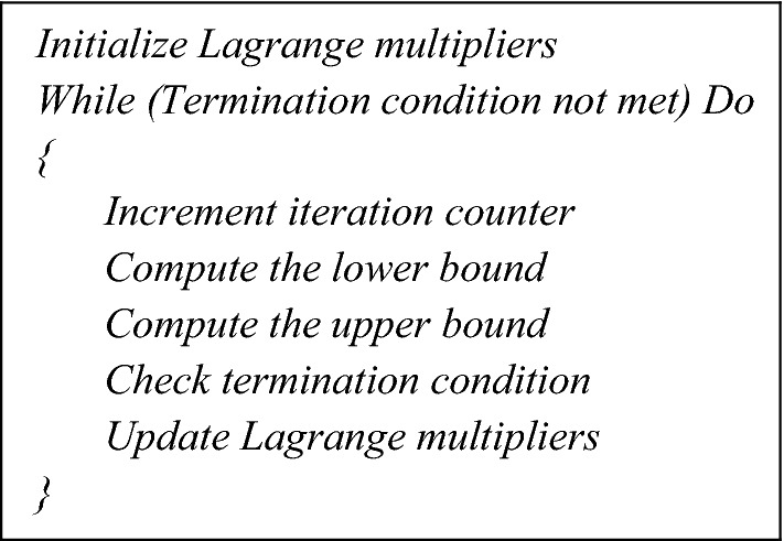
The main steps of Lagrangian relaxation (Lim et al. 2010)

The steps of algorithm are described in detail in the following sub-sections.

Computation of lower bound

The first step is to compute the lower bound. For fixed values of the Lagrange multipliers ${\lambda }_{\mathit{il}}$, (59) provides a lower bound on the optimal objective function (52), which is the linear reformulation of objective (1). Two methods are applied to generate lower bounds: in the first one, lower bounds are derived by solving the relaxed programming model (LRCDL) via exact algorithms, while in the second method, a fast-approximate approach is used to provide lower bounds based on Cui et al. (2010). Considering these two methods of obtaining lower bound, two Lagrangian relaxations are proposed.

An approximate model to find lower bound

Although in the exact model (LRCDL) one constraint has been relaxed, its worst-case complexity is still exponential. Thus, in this section we provide a fast approximate formulation and algorithm to find lower bounds in polynomial time. Inspired by Cui et al. (2010), we replace the variable probabilities P_lir, PP_lr and Pr_ijr with fixed numbers in the approximate formulation. Define i₁, i₂, …, i_I as the order of cross-docks such that $q_{i_1}\le q_{i_2}\le \cdots \le q_{i_I}$. In the case of identical q_i, the tie can be broken arbitrarily. For $1\le r\le \left|R\right|$, we replace P_lir with ƒ_r and PP_lr with ${\partial }_r$, where ƒ_r and ${\partial }_r$ are computed using Eqs. (66) and (67).

$$f_r=\left(1-q_{i_r}\right)\prod _{l=1}^{r-1}{q}_{i_l}$$ 66

$${\partial }_r=\prod _{l=1}^{r-1}{q}_{i_l}=\frac{f_r}{\left(1-q_{i_r}\right)}$$ 67

It should be noted that disruption probability for direct shipment is equal to zero and we do not consider it in ranking of cross-docks; the ranking is only done for cross-docking centers. Hence, if direct shipment is used for a supplier in level r, we can simply set $q_{i_r}=0$ and as a result $f_{r+1}=f_{r+2}=\cdots =f_R=0$. The Probability that plant j is served by cross-dock i at level r (Pr_ijr) also can be replaced by $f_r$. Equation (68) calculates the penalty of not serving a supplier at all. Regarding the above description, if there is direct shipment in any level of reassignment, the penalty cost will be zero.

$$\beta =\prod _{l=1}^R{q}_{i_l}$$ 68

Based on these modifications, the mathematical formulation will change to a linear programming model. The approximated model (CDL-APRX) is presented below.

$$\begin{array}{cc}& \left(\text{CDL}-\text{APRX}\right)\hfill \\ \hfill & Min\sum _{i\in I}{g}_i\times y_i+\sum _{r\in R}\sum _{j\in J}\sum _{l\in L}{c}_{\mathit{lj}}\times {\partial }_r\times U_{\mathit{ljr}}+\sum _{r\in R}\sum _{i\in I}\sum _{l\in L}{c}_{\mathit{li}}\times m_{\mathit{lir}}\times f_r\hfill \\ \hfill & +\sum _{r\in R}\sum _{i\in I}\sum _{l\in L}\sum _{j\in J}{v}_i\times d_{\mathit{jl}}\times B_{\mathit{lijr}}\times f_r+\sum _{r\in R}\sum _{i\in I}\sum _{l\in L}{c}_{\mathit{ij}}\times n_{\mathit{ijr}}\times f_r+\sum _{l\in L}^{}\beta \times {\gamma }_l\hfill \\ \hfill \end{array}$$ 69

$$\begin{array}{cc}& \text{Subject to}\hfill \\ \hfill & \left(2\right)-\left(8\right)\hfill \\ \hfill & \left(16\right)-\left(17\right)\hfill \\ \hfill \end{array}$$

Computation of upper bound

At each iteration of Lagrangian relaxation, both a lower and an upper bound are obtained. The solution of relaxed model (LRCDL) provides a lower bound. If it is feasible for original model (CDL-LP), then it provides an upper bound as well, and in fact an optimal solution for (CDL-LP): since the violation of constraint (3) is 0 and the lower and upper bounds are equal. If the solution of (LRCDL) is not feasible for (CDL-LP), then we construct a feasibility phase by the method that will be explained. Upper bounds are computed using the following process:

First, the decision variables are recalled from the lower bound solution and set as a parameter in programming model (CDL-LP). Then the feasibility of solution is checked regarding constraint set (3). In this procedure after finding a lower bound, the algorithm checks if the solution is feasible or not and if it is not, a modification on solution is executed. In order to do so, a loop is defined in which the following process is done.

$$\begin{array}{cc}& for\left(i,l\right)\hfill \\ \hfill & if\sum _{r\in R}^{}{Z}_{\mathit{ilr}}>0\&y_i=0;then{y}_i=1\hfill \\ \hfill & \mathit{end}\hfill \\ \hfill \end{array}$$

In order to strengthen the upper bound, another loop is defined that performs as a cutting constraint: if a cross-dock serves no supplier in all levels, it must be closed.

$$\begin{array}{cc}& for\left(i\right)\hfill \\ \hfill & if\sum _{r\in R}^{}\sum _{l\in L}{Z}_{\mathit{ilr}}=0\&y_i=1;then{y}_i=0\hfill \\ \hfill & \mathit{end}\hfill \\ \hfill \end{array}$$

After implementing this phase, we compute the upper bound for the original objective function (52) using the decision variables.

Multiplier initialization and updating

The Lagrange multipliers, λ, are initialized by setting their initial values to 2 (${\lambda }_{\mathit{il}}^{\left(0\right)}=2$). As mentioned before, each value of λ provides a lower bound on the optimal objective value of (CDL-LP). Thus, in order to find the best possible lower bound which is close to optimal value, we need to solve max obj(λ).

This problem is solved approximately using sub-gradient optimization as described by Fisher (1981, 1985) and Daskin (1995). At iteration n, the step size ${\tau }^{\prime n}$ is calculated by Eq. (70), where $\overline{\mathit{UB}}$ is the best known upper bound and $\mathit{LB}$ is the lower bound found at the current iteration. ${\rho }^n$ is a constant at iteration n, halved when 10 consecutive iterations fail to improve, and ${\rho }^1$ is initialized to 2. Using the lower and upper bounds obtained, the multipliers are updated based on Eq. (71).

$${\tau }^{\prime n}=\frac{{\rho }^n\left(\overline{\mathit{UB}}-LB\right)}{{\sum }_{i\in I}{\sum }_{l\in L}{({\sum }_{r\in R}{Z}_{\mathit{ilr}}-y_i)}^2}$$ 70

$${\lambda }_{\mathit{il}}^{\left(n+1\right)}=max\left\{0,{\lambda }_{\mathit{il}}^{\left(n\right)}+{\tau }^{\prime n}\left(\sum _{r\in R}{Z}_{\mathit{ilr}}-y_i\right)\right\}$$ 71

Termination criteria

The algorithm terminates when any of the following criteria is achieved:

1. $\frac{\overline{\mathit{UB}}-LB}{\mathit{LB}}<\epsilon$, in which $\epsilon$ is the pre-specified optimality tolerance (the gap between the best lower and upper bound gets close to zero); we typically set the tolerance value $\epsilon$ to 0.001;

2. The number of iterations reaches a maximum value determined by the user (i.e., n > n_max) or the maximum computing time is obtained;

3. Step size constant ${\rho }^n$ gets close to zero; i.e., ${\rho }^n<{\rho }_{\mathit{min}}$, which means that a negligible change in the solution configuration is detected. We typically set the minimum level of step size constant (${\rho }_{\mathit{min}}$) to 0.0001.

Computational results

Although there are some data sets in Snyder and Daskin (2005) and Lim et al. (2010) to evaluate the formulation and algorithm, the network and environment in our problem is different from these earlier studies. In our case, we consider a three-echelon supply chain regarding cross-docking networks and take in to account location and transportation problems, simultaneously, while they design a two-echelon reliable location problem. Thus, the geographical distribution of suppliers and assembly plants (i.e. the distance between them) is inspired by test problems considered by Hasani Goodarzi and Zegordi (2016): set 1(10 3 1) (i.e. 10 part suppliers, 3 cross-docks and 1 assembly plant), set 2 (17 5 2), set 3 (24 6 3), set 4 (30 8 4). For each problem set, we generate 10 instances (totally 40 instances). Distances between each couple of nodes are drawn from U (10, 100). Transportation cost is set equal to the distance between each couple of nodes. The maximum capacity of vehicles is assumed 100 and demand of assembly plants is drawn from U [20, 90] and rounded to the nearest integer. The penalty for not serving supplier l is set to 10³ for all suppliers in which losing a supplier is extremely costly. Fixed cost of establishing cross-docks is randomly generated from U (200, 500) and variable cost per commodity unit at all cross-docks is 0.01. Disruption probabilities q_i are drawn from U [0.1, 0.5].

We test the algorithm for |R| = 2, in all problem sets and for R = 3 and 4 in problem set 1. Using the programming formulation, the maximum capacity of cross-docks is obtained considering disruption risk for candidate nodes. The Lagrangian relaxation algorithm is coded in GAMS/CPLEX software (version 24.7) and run on a PC with an Intel Core 5 Duo CPU (2.33 GHz) and 2 GB memory. Parameter values for the algorithm are summarized in Table 3.

Table 3.

Parameter values for Lagrangian relaxation

Parameter	Value
Optimality tolerance	0.001
Maximum number of iterations	200
Initial value of $\rho$	2
Number of non-improving iterations before halving $\rho$	10
Minimum value of $\rho$ (${\rho }_{\mathit{min}}$)	10–4
Initial value of ${\lambda }_{\mathit{il}}^{}$	2

Algorithm performance

This section presents the results of computational study to investigate the performance of solution algorithms. We execute the Lagrangian relaxation process in two different methods: in the first one, lower bounds are obtained by solving the relaxed formulation via exact algorithm (LR1), and the second method (LR2) uses an approximate lower bound as described in Sect. 4.2.1.

For all problem sets, LR1 and LR2 are executed with heterogeneous disruption probabilities. Table 4 presents the result of solving four problem sets using GAMS/CPLEX, LR1 and LR2 in |R| = 2 levels. The third column shows the solutions found by GAMS/CPLEX, which are optimal in problem sets 1–3. For problem set 4, it is not able to find optimal solution in < 2 h and the solution reported in this table are the best solution found in 16 min. In Table 4, LB, UB and Gap give the lower bound, upper bound and gap between lower bound and upper bound in percent, respectively. The columns specified by “ITR” indicate the iteration number, when the best lower bound is reached for LR1 and LR2.

Table 4.

Algorithms’ results for two levels

Problem #	Level	CPLEX	LR1				LR2				CPU time (s)
			LB	UB	Gap (%)	ITR	LB	UB	Gap (%)	ITR	CPLEX	LR1	LR2
1	2	415.5	415.5	415.5	0.000	11	415.5	415.5	0.000	15	2	466	6
2	2	398.3	398.3	398.3	0.000	17	398.3	398.3	0.000	9	0.5	87	3
3	2	696.0	693.9	696.2	0.331	13	660.7	661.7	0.159	8	1	29	24
4	2	506.4	506.4	506.4	0.000	18	506.4	506.4	0.000	18	0.5	46	5
5	2	570.1	570.1	570.1	0.000	12	570.1	570.1	0.000	11	0.2	24	21
6	2	479.0	479.0	479.0	0.000	7	479.0	479.0	0.000	6	0.5	38	2
7	2	618.9	604.9	633.5	4.728	13	537.2	538.1	0.172	9	0.4	1061	24
8	2	450.5	450.5	450.5	0.000	18	450.5	450.5	0.000	19	0.5	116	5
9	2	591.7	591.7	591.7	0.000	13	574.2	591.7	3.040	13	0.5	63	4
10	2	587.3	587.1	587.3	0.034	14	583.8	583.8	0.000	17	0.7	1002	23
11	2	730.9	723.4	741.1	2.447	29	720.0	740.6	2.865	38	13	3196	35
12	2	869.3	845.5	907.6	7.345	20	864.5	892.2	3.212	87	6	382	66
13	2	885.5	885.5	885.5	0.000	87	866.5	884.5	2.084	36	26	1743	55
14	2	1004.4	993.12	1061.9	6.926	21	981.3	1023.1	4.263	48	56	5168	58
15	2	1104.1	1087.4	1120.9	3.081	49	1103.3	1167.9	5.855	92	6	3497	54
16	2	1031.8	1020.9	1107.6	8.493	96	1019.0	1060.3	4.056	99	4	2964	55
17	2	1161.1	1149	1196.1	4.099	38	1126.1	1201.2	6.669	52	11	4215	29
18	2	1016.4	1014.9	1053.9	3.843	44	1007.3	1048.4	4.086	105	18	5109	52
19	2	1095.0	1091.8	1145.1	4.882	51	1090.9	1134.9	4.035	51	6	4238	44
20	2	1219.9	1204	1253.8	4.136	37	1189.7	1234.8	3.784	54	108	9481	59
21	2	2873.1	2861.3	2885.6	0.849	41	2949.5	2987.7	1.295	95	246	71,876	98
22	2	3008.2	NA**	NA	–	–	2792.7	2850.0	2.052	90	411	–	78
23	2	2934.2	NA	NA	–	–	2811.8	2829.9	0.642	45	435	–	76
24	2	2921.8	NA	NA	–	–	2809.4	2825.4	0.568	58	428	–	81
25	2	2867.5	NA	NA	–	–	2657.5	2734.3	2.890	22	247	–	85
26	2	2613.4	NA	NA	–	–	2591.8	2626.2	1.326	11	52	–	88
27	2	3040.6	NA	NA	–	–	2964.1	2992.0	0.944	80	302	–	90
28	2	2617.3	NA	NA	–	–	2561.5	2712.3	5.885	96	197	–	90
29	2	3176.6	NA	NA	–	–	3080.2	3197.1	3.793	78	354	–	77
30	2	2873.4	NA	NA	–	–	2791.6	2810.5	0.676	111	261	–	98
31	2	6059.0*	NA	NA	–	–	5393.7	5430.4	0.679	97	960	–	150
32	2	5474.4*	NA	NA	–	–	4791.9	4867.2	1.572	161	960	–	270
33	2	6305.0*	NA	NA	–	–	4605.0	4765.4	3.483	85	960	–	283
34	2	6159.0*	NA	NA	–	–	4547.8	4653.3	2.319	72	960	–	702
35	2	6173.8*	NA	NA	–	–	4991.5	5161.7	3.410	126	960	–	627
36	2	5519.8*	NA	NA	–	–	4907.0	4946.3	0.801	72	960	–	750
37	2	6763.0*	NA	NA	–	–	5348.3	5469.2	2.260	190	960	–	604
38	2	6374.0*	NA	NA	–	–	4959.1	5088.2	2.603	168	960	–	459
39	2	6191.5*	NA	NA	–	–	4902.7	5105.2	4.132	151	960	–	360
40	2	4756.6*	NA	NA	–	–	4355.4	4393.5	0.875	52	960	–	487

*The solutions are not optimal, but the best possible solution found in 16 min

**NA not available

For problem #21, the gap between lower and upper bound of LR1 is small (0.849%), though LR1 took about 20 h to solved it. Hence, problem set 3 and 4 do not have available solution using LR1 as the solving method. For problem set 1–3, the optimal solutions are available, so Table 5 shows the difference between lower bound of LR2 and optimal solution in problem #1 to #30. These values are shown in GAP columns. LR2 is able to find optimal solutions in 6 cases of problem set 1. Although there is a gap between its lower bound and optimal solution, it is fast compared to exact method regarding Table 4.

Table 5.

The difference between optimal value and lower bound of LR2

Problem #	GAP (%)	Problem #	GAP (%)	Problem #	GAP (%)
1	0.000	11	1.494	21	1.953
2	0.000	12	0.561	22	2.799
3	5.076	13	2.150	23	4.171
4	0.000	14	2.305	24	3.846
5	0.000	15	0.077	25	7.323
6	0.000	16	1.241	26	0.826
7	13.205	17	3.017	27	2.517
8	0.000	18	0.895	28	2.132
9	2.950	19	0.378	29	3.035
10	0.602	20	2.475	30	2.845
Average	2.183	Average	1.460	Average	3.145

As can be inferred from Table 4, in some instances like problem #3, LR2 presents a small gap between lower and upper bound, while it has a considerable difference with optimal value. This happens because of reformulation of model in LR2 and solving an approximate model to find lower bound. Similarly, in problem #10 the lower and upper bounds of LR2 are equal but with a deviation from CPLEX solution. In such cases, LR2 finds equal lower and upper bounds and consequently an optimal solution for the approximated model that has a deviation from the original model (CDL-LR).

The difference of solutions found by LR2 and CPLEX is relatively large in set 4, since in this problem set CPLEX solutions are not optimal and consequently are greater than optimal value, so the difference between approximated lower bound and CPLEX solutions is considerable. Regarding Table 5, in problem set 3, the difference between CPLEX and LR2 is great compared to other sets, though the lower and upper bound of this algorithm has a relatively small gap.

In Table 4, two levels of reassignment are considered. In order to study the effect of levels on solutions quality and computational time, problem set 1 is solved with |R| = 3 and 4 levels in Table 6. It should be noted that in most cases, computational time drastically grows when the number of levels increases, but it is not necessarily more in four-level problems compared to three-level instances. This trend is true for most problem instances, even in the cases that solution structure and cost are the same for |R| = 2, 3 and 4 levels. The computation time of LR1 for more complicated problems is considerably high, for instance, CPU time for problem #11 is about 7 h and 54 min when there are 3 levels of reassignment. Algorithm LR1 is not able to solve problem #11 in less than 28 h with R = 4. CPLEX solves it in 125 s for |R| = 3 and we set a time limitation of 16 min for |R| = 4. Only the results for set 1 are reported in Table 6.

Table 6.

Results of solving problem set 1 with 3 and 4 levels of reassignment

Problem #	Level	CPLEX	LR1				LR2				CPU time (s)
			LB	UB	Gap (%)	ITR	LB	UB	Gap (%)	ITR	CPLEX	LR 1	LR2
1	3	415.5	415.5	415.5	0.000	16	415.5	415.5	0.000	15	0.7	570	6
	4	415.5	415.5	415.5	0.000	19	415.5	415.5	0.000	15	1	592	7
2	3	398.3	398.3	398.3	0.000	23	398.3	398.3	0.000	9	1	614	5
	4	398.3	398.3	398.3	0.000	21	398.3	398.3	0.000	9	2	745	4
3	3	729.2	731.5	731.5	0.315	13	701.8	710.8	1.291	6	5	959	30
	4	729.2	729.2	729.22	0.000	24	701.8	710.8	1.291	5	6	1260	28
4	3	506.4	506.4	506.4	0.000	3	506.4	506.4	0.000	15	0.7	25	6
	4	506.4	506.4	506.4	0.000	3	506.4	506.4	0.000	15	1	62	6
5	3	570.1	570.1	570.1	0.000	12	570.1	570.1	0.000	12	1	24	24
	4	570.1	570.1	570.1	0.000	60	570.1	570.1	0.000	12	1	152	25
6	3	479.0	479.0	479.0	0.000	6	479.0	479.0	0.000	6	0.9	72	3
	4	479.0	479.0	479.0	0.000	4	479.0	479.0	0.000	6	1	1006	3
7	3	618.9	618.9	618.9	0.000	10	537.2	538.1	0.172	9	0.9	358	30
	4	618.9	592.6	701.3	18.343	14	537.2	538.1	0.172	9	1	1263	29
8	3	450.5	450.5	450.5	0.000	14	450.5	450.5	0.000	15	0.9	99	7
	4	450.5	450.5	450.5	0.000	9	450.5	450.5	0.000	15	1	1525	7
9	3	591.7	591.7	591.7	0.000	67	591.7	591.7	0.000	13	0.9	1033	5
	4	591.7	591.7	591.7	0.000	13	591.7	591.7	0.000	13	1	1026	5
10	3	587.4	559.4	587.4	5.005	16	586.1	598.8	2.165	17	1	1367	16
	4	587.4	563.4	587.5	4.278	24	586.1	598.8	2.165	17	2	361	27

When the costs of problem set 1 are scrutinized in Tables 4 and 6, in most cases increasing the number of levels does not change the objective value. This event has a simple reason: in this problem set, either all shipments are moved directly in the first level or a cross-dock is used in the first level and direct shipment in the second level. Since it is not cost-effective to open more than one cross-dock, the model decides to send every consignment directly or use at most one cross-dock. If model assigns the only cross-dock to nodes in a level, in the next level it will use direct shipment definitely. When the direct shipment is assigned in a level, no cross-docking center will be allocated in the next level as a backup method for direct shipment, meaning that problem will be solved in one or two levels and increasing the reassignment level will not change the solution in such kind of instances. Moreover, in the cases when only direct shipment is used, the result is the same for LR1 and LR2 and increasing the number of levels will not change the cost, but CPU time in most cases drastically grows especially in LR1. As an example, in problem #6, CPU time for |R| = 4 is considerably more than that of 2 and 3 levels. In problem #7 with |R| = 2, although all shipments are implemented by direct strategy, LR1 is not able to find optimal solution and takes considerable computation time, while for |R| = 3 it finds optimal solution in a less running time.

As mentioned in the literature, heterogeneous disruption probability makes the model very complicated, while for problems with identical probability, CPLEX is able to find optimum solution in a small amount of running time. For illustration, CPU time of CPLEX for problem #21 to #25 is reported in Fig. 3 in two cases: with identical and heterogeneous disruption probability.

Fig. 3.

A comparison of CPLEX CPU time (s) in cases of identical and heterogeneous for test problem #21 to #25

In general, some points can be easily inferred from the results, LR1 takes more CPU time compared to LR2 and CPLEX (optimal solution). LR1 is not able to solve problem set 3 in less than 20 h, thus we solve set 3 and set 4 just by CPLEX and LR2. CPU time of LR2 is less than that of CPLEX, especially in set 4. Moreover, penalty cost is set to 10³ for all suppliers and in none of instances, penalty cost happens.

Case study

In this section, we present the application of the approach on a real industrial case in auto-making industry. The chosen case is the biggest auto-making company in the Middle East consisting of more than 600 suppliers in different cities. To simplify the problem, we categorize all suppliers in 24 different cities. There are five assembly plants and six potential locations for establishing cross-dock(s). Location of all nodes in this distribution network can be found in “Appendix 3”. Transportation cost between each couple of nodes is shown in “Appendix 3”, as well. The homogenous vehicle fleet consists of trucks and capacity of each truck is 192 standard pallets. The smallest pallet is defined as the standard pallet in the real case and size of other pallets are reported in comparison with the standard pallet.

In order to estimate the fixed cost of establishing cross-docks, we utilize the approach developed by Gumus and Bookbinder (2004), in which, the establishing (commissioning) cost is determined per each usage. Based on experts in the company, estimated establishing cost is about 3 million dollars. If depreciation period of cross-docks is set to 12 years, the annual establishing cost is $250,000. Regarding similar cases in auto-making industry, shipments typically spend less than 72 h in the cross-docking process (3 days). Hence, the prorated establishing cost is about $2083 for each time of utilization (around ten times a month). We simply put $2500 for this cost. As mentioned above, the time frame of the model is set to 72 h, which is equivalent to each time of running the cross-docking process, from the first step (pick up parts from suppliers) to the last point (drop parts off at assembly plants). This time interval is based on the case study and other similar real cases data in auto making industry for which the data of transportation costs are defined in 3 days intervals. That is why all costs including fixed cost of establishing cross-docks are transformed to be used in this time scope. We note that this transformation can be done with any length of time frame, depending on the case study data. Operational cost at cross-docks is calculated based on number of standard pallets passing through them and is set to $0.25 for each pallet. The potential nodes to establishing cross-docks are: Nodes 25, 26, 27, 28, 29 and 30, as can be found in Fig. 7 in “Appendix 3”.

Fig. 7.

The geographical distribution of suppliers, potential cross-docks and assembly plants

Case without disruption

First, the problem is solved under normal condition without considering disruption to indicate the effect of using cross-docking on total distribution cost. Based on case study conditions, the demand from a supplier can be more than vehicle capacity, hence, we modified the objective function as follows.

$$\begin{array}{cc}& Min\sum _{i\in I}{g}_i\times y_i+\sum _{r\in R}\sum _{j\in J}\sum _{l\in L}{c}_{\mathit{lj}}\times di{r}_{\mathit{ljr}}+\sum _{r\in R}\sum _{i\in I}\sum _{l\in L}{c}_{\mathit{li}}\times m_{\mathit{lir}}\hfill \\ \hfill & +\sum _{r\in R}\sum _{i\in I}\sum _{l\in L}\sum _{j\in J}{v}_i\times d_{\mathit{jl}}\times B_{\mathit{lijr}}+\sum _{r\in R}\sum _{i\in I}\sum _{l\in L}{c}_{\mathit{ij}}\times n_{\mathit{ijr}}\hfill \\ \hfill \end{array}$$ 72

Constraint (73) has been also added to the model.

$$U_{\mathit{ljr}}\times d_{\mathit{jl}}\ge di{r}_{\mathit{ljr}}\times Q;\forall l,j,r$$ 73

where $di{r}_{\mathit{ljr}}$ is the number of vehicles that go directly from supplier l to plant j at level r. When both strategies (direct shipment and cross-docking) are allowed, cost terms are as indicated in Table 7.

Table 7.

Terms of supply cost when both strategies are allowed

Cost type	Value ($)
Fixed cost of establishing cross-dock	2500
Direct transshipment cost	8607
Indirect transportation cost from suppliers to CDs (pick up cost)	8450
Indirect transportation cost from CDs to plants (delivery cost)	8515
Variable cross-docking cost at receiving process	1060
Total cost	29,132

In this solution, City 30 is selected as cross-dock, for which the best capacity is 4240 pallets. This means that if we consider totally 10,000 pallets in the system, 42.39% of pallets go through cross-dock and the remaining are sent directly. Total number of vehicles from cross-dock to assembly plants 1 to 5 is 9, 6, 1, 1 and 7, respectively. Totally 41 vehicles are sent directly from suppliers to assembly plants. If we force the model to pass all transshipments through cross-dock, the total cost of system will be $33,247, for which the cost terms are shown in Table 8. In this case, City 30 is selected for setting up the cross-dock, as well, with the capacity of 10,000 pallets. If creating such a capacity is not possible, more than one cross-dock should be established. In contrast, if all shipments have to be done directly, total cost of network is $58,003. If limited capacity of vehicles is relaxed, the total number of pallets passing thought cross-docks will be 6134 which means that in a network with this topology, considering a combination of both strategies is economical and for 61.34% of pallets, at maximum, cross-docking strategy is recommended.

Table 8.

Terms of supply cost when just cross-docking is allowed

Cost type	Value ($)
Fixed cost of establishing cross-dock	2500
Direct transshipment cost	0
Indirect transportation cost from suppliers to CDs (pick up cost)	14,699
Indirect transportation cost from CDs to plants (delivery cost)	13,549
Variable cross-docking cost at receiving process	2499
Total cost	33,247

In order to investigate the effect of cross-docks capacity on total cost, we boost the capacity from 1000 pallets to 10,000 pallets. The result is indicated in Fig. 4. It seems that capacity of 4000 pallets is an appropriate choice, which decrease 21% of cost, in comparison with capacity of 1000 pallets. The fluctuation in trend may be because of CPLEX solver which is sensitive to large values such as big M.

Fig. 4.

The effect of cross-dock capacity on total supply cost

Case considering disruption

In this sub-section the problem is solved in the condition in which the probability of disruption is counted. As mentioned in the literature, a drawback of this approach is assuming known disruption probabilities (Jabbarzadeh et al., 2016), while cross-dock failure probabilities, q_i, should be estimated by historical data, experts view and some other resources such as the probability of earthquake, fire and flood occurrence in a region. “Since historical data on rare events such as earthquakes, floods, strikes, and terrorist attacks are limited or nonexistent, the likelihood of a disruption occurrence is difficult to quantify” (Simchi-Levi et al. 2014). Because of lacking historical data in disruption occurrence, we consider the same probability of disruption in all potential cross-docks, which is one limitation of our work. The objective function of model is modified to Eq. (74).

$$\begin{array}{cc}& Min\sum _{i\in I}{g}_i\times y_i+\sum _{r\in R}\sum _{j\in J}\sum _{l\in L}{c}_{\mathit{lj}}\times di{r}_{\mathit{ljr}}\times q^{r-1}+\sum _{r\in R}\sum _{i\in I}\sum _{l\in L}{c}_{\mathit{li}}\times m_{\mathit{lir}}\left(1-q\right)q^{r-1}\hfill \\ \hfill & +\sum _{r\in R}\sum _{i\in I}\sum _{l\in L}\sum _{j\in J}{v}_i\times d_{\mathit{jl}}\times B_{\mathit{lijr}}\left(1-q\right)q^{r-1}+\sum _{r\in R}\sum _{i\in I}\sum _{l\in L}{c}_{\mathit{ij}}\times n_{\mathit{ijr}}\left(1-q\right)q^{r-1}+\sum _{l\in L}^{}{q}^R{\gamma }_l\hfill \\ \hfill \end{array}$$ 74

To investigate the influence of factors on cost and number of opened cross-docks, sensitivity analysis is performed here in four various aspects:

• The effect of fixed cost of establishing cross-docks on total cost of network

• The effect of disruption probability on total cost of network

• The effect of number of recovery levels (R) on total cost of network

• The effect of not servicing penalty on total cost of network

The effect of fixed cost of establishing cross-docks on total cost of network

In the first run, q is 0.1 for all cross-docks and |R| = 2. Penalty cost of not serving is set to $250 and fixed cost of establishing is $2500. In this problem, City 30 is chosen for setting up the cross-dock, as in previous section. Totally, 3384 pallets pass through it. Other details are provided in Table 9.

Table 9.

Terms of supply cost when disruption is considered (|R| = 2, Fixed cost of establishing = $2500)

Cost type	Value ($)
Fixed cost of establishing cross-dock	2500
Direct transshipment cost	15,631
Indirect transportation cost from suppliers to CDs (pick up cost)	7298
Indirect transportation cost from CDs to plants (delivery cost)	6363
Variable cross-docking cost at receiving process	846
Penalty cost of not servicing	0
Total cost	32,638

When prorated establishing cost of each potential cross-dock is $5000, City 30 still is chosen with the best capacity of 4212 pallets. Details of this run is presented in Table 10.

Table 10.

Terms of supply cost when disruption is considered (|R| = 2, Fixed cost of establishing = $5000)

Cost type	Value ($)
Fixed cost of establishing cross-dock	5000
Direct transshipment cost	11,819
Indirect transportation cost from suppliers to CDs (pick up cost)	7975
Indirect transportation cost from CDs to plants (delivery cost)	8592
Variable cross-docking cost at receiving process	1053
Penalty cost of not servicing	0
Total cost	34,439

In order to investigate this sensitivity, various runs of problem with different values for establishing cost, from 2500 to 40,000 are performed, whose result are shown in Table 11 and Fig. 5.

Table 11.

The effect of changing fixed cost of establishing cross-docks on total system cost (|R|  = 2)

Fixed cost of establishing each cross-dock ($)	Total cost ($)	Number of pallets	Chosen cross-dock
2500	32,638	3384	City 30
5000	34,439	4212	City 30
7500	36,873	4077	City 30
10,000	41,238	3110	City 30
12,500	41,670	4193	City 30
15,000	44,448	4255	City 30
17,500	46,948	4255	City 30
20,000	49,438	4211	City 30
22,500	51,948	4255	City 30
25,000	55,188	3033	City 30
27,500	57,393	3571	City 30
30,000	60,093	3223	City 30
32,500	63,803	–	–
35,000	63,803	–	–

Fig. 5.

Trend of total system cost relative to changing in fixed cost of establishing cross-docks (|R| = 2)

Having used Newton's method, we found the first point at which all transshipments are done directly from suppliers to assembly plants. In other words, the set point for direct shipment and cross-docking is the point in which prorated fixed cost of establishing cross-dock is $30,275 at maximum.

The effects of disruption probability and number of recovery levels |R| on total cost of network

In this run, fixed cost of establishing each cross-dock is $2500 and not servicing penalty for each supplier is $2500, meaning that parts shortage is not allowed. In order to observe the effects of increasing levels and disruption probability on the total cost, we solve the problem with different values for R and q. q is varied between 0.1 to 0.5 with the step size of 0.05 and R = 2, 3, 4. The results are indicated in Table 12 and Fig. 6.

Table 12.

The sensitivity of total cost to parameter q and R

q	Two levels			Three levels			Four level
	Obj value	No. of CD	No. Pr	Obj value	No. of CD	No. Pr	Obj value	No. of CD	No. Pr
0.1	31,562.5	2	4604	32,805	2	4290	32,282.5	2	4317
0.15	32,460	2	4560	33,157.5	2	4411	32,595	2	4391
0.2	34,675	2	4387	33,182.5	2	4617	34,697.5	2	4217
0.25	36,137.5	2	4429	35,505	2	4171	37,230	3	5021
0.3	37,045	2	4733	37,100	2	4644	36,690	3	5272
0.35	36,957.5	2	4860	36,712.5	2	4860	37,105	3	5686
0.4	39,282.5	2	5129	38,842.5	3	5428	40,385	3	5313
0.45	41,817.5	2	4696	42,140	4	5602	39,370	3	5615
0.5	44,672.5	2	4319	43,972.5	2	4584	42,767.5	3	5335

No. Pr number of pallets passing through cross-dock, No. of CnD Number of opened cross-docks

Fig. 6.

The effect of increasing q and R on total cost of problem (penalty cost of not servicing = $2500)

When |R| = 3 and q = 0.5, the solver decides to establish two cross-docking centers. Penalty cost in this test problem is 0, since it uses direct shipment as a backup strategy for all suppliers. Candidate nodes of 28 and 30 are chosen as cross-docks in all cases. For some values of q, other candidates are added to them. For instance, when |R| = 3 and q = 0.45, candidate nodes of 27 up to 30 are recommended by solver for establishing cross-docks.

In Fig. 6, we observe that the total cost is sensitive to disruption probability, and for a given probability of disruption, the impact of R is very low or even negligible. We also observe that, when the disruption is highly probable, higher levels of recovery plans become interesting to consider.

The effect of not servicing penalty on total cost of network

When |R| = 2, q = 0.2 and not servicing penalty cost for each supplier is $250, the total cost of network is $32,485 and 4287 pallets pass through cross-dock. Increasing this penalty cost from $250 to $15,000 leads to the results in Table 13. When penalty cost for each supplier is $9250, the solver prefers to use direct shipment as the main or back up strategy for all consignments and one node is chosen for setting up cross-dock. Total transportation cost is $38,143 and penalty cost is 0. In other words, if shortage of parts is not allowed and imposes a huge cost on system, direct movement is recommended as the main or backup strategy for all shipments. In this case, establishing cross-dock will be done in Node 27. Increasing penalty to extremely large values will not change the solution.

Table 13.

The sensitivity of total cost to changes in not-servicing penalty

Not-servicing penalty ($)	Total cost ($)	Number of pallets	Opened cross-dock
250	32,485	4287	Node 28, Node 30
1250	33,620	4676	Node 28, Node 30
2500	34,675	4383	Node 28, Node 30
3750	35,345	4373	Node 28, Node 30
5000	36,263	4220	Node 28, Node 30
6250	37,188	3648	Node 30
7500	37,628	3221	Node 30
8750	38,445	3890	Node 30
10,000	38,143	3751	Node 27
11,250	38,143	3751	Node 27
12,500	38,143	3751	Node 27
13,750	38,143	3751	Node 27
15,000	38,143	3751	Node 27

To sum up, the results show that in such networks, using cross-docking exclusively, is not the solution and for the chosen case, this can be used just for 61.34% of flow of parts, at maximum, when capacity of vehicles is relaxed. Hence, forcing all parts to pass through cross-docks is not cost effective. According to Tables 7 and 8, integrating both strategies can reduce system cost about 14% compared to condition in which only cross-docking is allowed. This approach also can diminish costs about 99% in comparison to exclusive direct shipment. In most runs, Node 30 is chosen as the best location to set up a cross-dock. The break-even point of fixed cost of establishing cross-dock is $30,275, meaning that the budget for commencing cross-dock can be $43,596,000 at maximum. Spending more than this amount is not economic. Regarding Fig. 4 (normal condition) and Table 12, the best capacity for cross-dock is proposed to be about 40% to 50% of total pallets in system. The exact value of capacity can be determined regarding fixed cost and other parameters.

Comparing the case with and without disruption (Tables 7, 9), we will find that considering failure probability of 0.1 for all cross-docks leads to 12% increase in the total cost. When there is no disruption in the system, 4240 pallets pass the cross-dock, while in disruption condition with q = 0.1, 3384 pallets go through cross-dock and direct shipment is preferred in comparison with normal situation. Hence, the required capacity of cross-dock is decreased. In both cases the same location is selected to open a cross-dock.

Paying attention to data of Table 12, one can realize that when |R| = 2 and shortage is not allowed, increasing disruption probability from 0.1 by 5% leads to 2.84% cost growth. Changing q from 0.1 to 0.2 causes 9.86% augmentation in total cost, while to 0.3 causes 17.4% cost increase. If failure probability raises from 0.1 to 0.5, there will be 41.5% increment in the total cost of system to handle this disruption risk. In these cases, two locations are chosen to establish cross-docks. Comparing the result in this table with Table 7 reveals that when there is 0.2 failure probability for all cross-docks, 19% more cost is imposed on the distribution system to handle the disruption risk (in comparison with normal condition).

Conclusion

Nowadays consequences of disruptions caused by natural disasters, terrorist attacks or man-made events on supply chains cannot be neglected. In order to deal with these consequences, one effective approach is to design recovery plans to apply in the case of disruptions. In this study we attempt to hedge against disruption in cross-docking facilities by considering levels of reassignment in which every supplier can be allocated to up to |R| ≥ 1 cross-docks. If disruption occurs, this supplier will be either diverted to other operational cross-docks or served by direct shipment as the backup strategy. This approach can be easily utilized in many supply chains having any kind of distribution centers (not necessarily the cross-docking centers), such as food, clothing and auto making industries, etc. We present a mathematical model for this problem to find cross-dock locations and the optimal capacity of them. In the model (CDL-NLP), the disruption probabilities are heterogeneous (facility-specific), which significantly complicates the mathematical model and makes it a nonlinear programming formulation. In order to solve the nonlinear model, first some tools are utilized to linearize it and generate (CDL-LP). Then we propose two Lagrangian relaxation-based methods (LR1 and LR2) that are effective for solving the linearized model. LR1 finds lower bounds by solving relaxed model via exact methods, while in LR2 an approximated model is utilized to estimate the lower bound quickly. Approximated solving method (LR2) provides near-optimal solutions for (CDL-LP) quickly (with an optimality gap below 2.26%) and handles larger problem instances compared to CPLEX and LR1. Computational studies for model (CDL-LP) show that LR2 is fast (in terms of CPU time) with a small optimality gap, while LR1 outperforms it in terms of solution quality.

A case study is conducted in this research on the biggest auto-making company in Middle East. We present some sensitivity analysis on the case to investigate the effect of changing various parameters on system cost and number of opened cross-docks. Based on results, in such networks, using cross-docking exclusively, is not a recommended solution and integrating cross-docks with direct shipment is cost-effective. Increasing disruption probability can impose a surplus cost on system and in most cases increments the number of opened cross-docks.

Appendix 1

The mathematical model for identical disruption in all cross-docks (Hasani Goodarzi et al. 2018).

$$\begin{array}{cc}& \left(\text{HDCDL}\right)\hfill \\ \hfill & Min\sum _{i\in I}{g}_i{y}_i+\sum _{r\in R}\sum _{j\in J}\sum _{l\in L}{c}_{\mathit{lj}}{U}_{\mathit{ljr}}{q}^{r-1}+\sum _{r\in R}\sum _{i\in I}\sum _{l\in L}{c}_{\mathit{li}}{m}_{\mathit{lir}}\left(1-q\right)q^{r-1}\hfill \\ \hfill & +\sum _{r\in R}\sum _{i\in I}\sum _{l\in L}\sum _{j\in J}{v}_i{d}_{\mathit{jl}}{B}_{\mathit{lijr}}\left(1-q\right)q^{r-1}+\sum _{r\in R}\sum _{i\in I}\sum _{l\in L}{c}_{\mathit{ij}}{n}_{\mathit{ijr}}\left(1-q\right)q^{r-1}\hfill \\ \hfill & +\sum _{l\in L}^{}{q}^R{\gamma }_l\hfill \\ \hfill \end{array}$$ 75

$$\begin{array}{cc}& \text{Subject}\text{to}\hfill \\ \hfill & U_{\mathit{ljr}}+\sum _{i\in I}{B}_{\mathit{lijr}}=1;\forall l,j,r\hfill \\ \hfill \end{array}$$ 76

$$\sum _{r\in R}^{}{Z}_{\mathit{ilr}}\le y_i;\forall i,l$$ 77

$$\sum _{j\in I}{B}_{\mathit{lijr}}\times d_{\mathit{jl}}\le m_{\mathit{lir}}\times Q;\forall l,i,r$$ 78

$$\sum _{l\in L}{d}_{\mathit{jl}}\times B_{\mathit{lijr}}-w_{\mathit{ijr}}=0;\forall i,j,r$$ 79

$$Z_{\mathit{ilr}}\le \sum _{j\in J}{B}_{\mathit{lijr}};\forall l,i,r$$ 80

$$\sum _{j\in J}{B}_{\mathit{lijr}}\le \left|J\right|\times Z_{\mathit{ilr}};\forall l,i,r$$ 81

$$w_{\mathit{ijr}}\le n_{\mathit{ijr}}\times Q;\forall i,j,r$$ 82

$$y_i,U_{\mathit{ljr}},B_{\mathit{lijr}},Z_{\mathit{ilr}}\in \left\{0,1\right\}$$ 83

$$m_{\mathit{lir}},n_{\mathit{ijr}},w_{\mathit{ijr}}\in \left\{0,1,2,\dots \right\}$$ 84

Appendix 2

The probability estimation in constraints (10)–(14), are more explained here. In constraint (10), the probability that cross-dock i serves supplier l at level r is counted using this concept: cross-dock i is operational $\left(1-q_i\right)$ and all assigned cross-docks in previous levels are non-operational.

$$\begin{array}{cc}\hfill P_{\mathit{lir}}& =\left(1-q_i\right)\times \left(\sum _{k=1}^I{q}_k\times Z_{klr-1}\right)\times \left(\sum _{\mathit{k}=1}^{\mathit{I}}{\mathit{q}}_{\mathit{k}}\times {\mathit{Z}}_{\mathit{klr}-2}\right)\hfill \\ \hfill & \times \cdots \times \left(\sum _{\mathit{k}=1}^{\mathit{I}}{\mathit{q}}_{\mathit{k}}\times {\mathit{Z}}_{\mathit{kl}1}\right);\forall l,i;2\le r\le \left|R\right|\hfill \\ \hfill \end{array}$$

The probability that cross-dock k serves supplier l at previous level r − 2 is as follows:

$$\begin{array}{cc}\hfill P_{lkr-1}& =\left(1-q_k\right)\times \left(\sum _{\mathit{k}=1}^{\mathit{I}}{\mathit{q}}_{\mathit{k}}\times {\mathit{Z}}_{\mathit{klr}-2}\right)\times \left(\sum _{\mathit{k}=1}^{\mathit{I}}{\mathit{q}}_{\mathit{k}}\times {\mathit{Z}}_{\mathit{klr}-3}\right)\hfill \\ \hfill & \times \cdots \times \left(\sum _{\mathit{k}=1}^{\mathit{I}}{\mathit{q}}_{\mathit{k}}\times {\mathit{Z}}_{\mathit{kl}1}\right);\forall l,k;2\le r\le \left|R\right|\hfill \\ \hfill \end{array}$$

So, by substitution the bold term, $P_{\mathit{lir}}$ can be rewrite as follows:

$$P_{\mathit{lir}}=\left(1-q_i\right)\times \left(\sum _{k=1}^I{q}_k\times Z_{klr-1}\right)\frac{P_{lkr-1}}{\left(1-q_k\right)}=\left(1-q_i\right)\times \sum _{k=1}^I\frac{q_k}{1-q_k}\times P_{lkr-1}\times Z_{klr-1}$$

In constraint (11), the probability that direct shipment serves suppliers at the first level is set to 1, since it is a reliable strategy. Constraint (12) is similar to constraint (10), when $\left(1-q_i\right)$ is equal to 1, since the failure probability of direct movement is considered 0.

Based on failure probability at cross-dock i and using constraint (10), we can simply determine the probability that this cross-dock serves supplier l at level r, while we also need to know the probability that this cross-dock serves a plant. In constraint (13), the probability that cross-dock i serves plant j at level r is counted. In order to do so, a weighted average of all demands of plant j which pass thought cross-dock i is utilized, where the probability of using this cross-dock is the weight. In the denominator, all products which are sent to this plant through this cross-dock is used. In order to avoid cases with denominator equal to zero (when cross-dock i does not send any product to plant j), we add $\epsilon$ to the denominator.

In constraint (14), the probability that a supplier will not be served at all is calculated, which means that at the last level, |R|, and all previous levels, the assigned cross-docks are disrupted, and there is no cross-dock to serve this supplier. If direct shipment is assigned to a supplier at a level $1\le r\le \left|R\right|$, this probability will be zero, since direct shipment is a secure method to move products.

Appendix 3

See Fig. 7 and Tables 14, 15 and 16.

Table 14.

Transportation cost from suppliers to plants ($)

Suppliers	Assembly plants
	Plant 5	Plant 5	Plant 5	Plant 5	Plant 5
City 1	227	576	66	603	471
City 2	256	546	300	600	690
City 3	227	576	66	603	471
City 4	210	576	66	625	438
City 5	497	653	603	66	774
City 6	465	510	504	366	729
City 7	550	705	613	343	600
City 8	113	473	363	471	567
City 9	570	615	553	351	588
City 10	498	687	471	774	66
City 11	267	555	368	600	414
City 12	319	555	395	600	383
City 13	475	681	471	774	75
City 14	463	585	471	774	128
City 15	135	350	369	503	653
City 16	150	343	387	525	666
City 17	131	366	339	478	644
City 18	414	150	576	653	687
City 19	101	462	351	495	570
City 20	198	336	423	615	671
City 21	66	396	330	528	528
City 22	75	444	306	546	489
City 23	85	444	306	546	489
City 24	63	414	312	497	498

Table 15.

Transportation cost from suppliers to potential cross-docks ($)

Suppliers	Potential nodes for establishing cross-docks
	Node 25	Node 26	Node 27	Node 28	Node 29	Node 30
City 1	491	471	318	268	576	263
City 2	480	690	507	131	546	244
City 3	501	471	318	278	576	272
City 4	530	438	185	316	576	309
City 5	362	774	613	720	653	599
City 6	50	729	426	354	510	236
City 7	467	600	739	800	705	682
City 8	206	567	225	218	473	59
City 9	240	588	462	542	615	422
City 10	729	66	387	644	687	570
City 11	426	414	87	372	555	315
City 12	522	383	143	418	555	401
City 13	767	75	363	689	681	579
City 14	684	128	339	605	585	588
City 15	355	653	323	27	350	118
City 16	386	666	360	65	343	148
City 17	354	644	372	50	366	117
City 18	510	687	555	366	150	462
City 19	236	570	315	117	462	50
City 20	456	671	417	133	336	227
City 21	347	528	312	75	396	107
City 22	290	489	218	153	444	132
City 23	342	489	252	143	444	133
City 24	465	498	267	131	414	101

Table 16.

Transportation cost from cross-docks to plants ($)

Cross-docks	Assembly plants
	Plant 1	Plant 2	Plant 3	Plant 4	Plant 5
Node 25	465	510	504	366	729
Node 26	498	687	471	774	66
Node 27	267	555	368	600	414
Node 28	131	366	339	478	644
Node 29	414	150	576	653	687
Node 30	101	462	351	495	570

Compliance with ethical standards

Conflict of interest

The authors declare that they have no conflict of interest.

References

- Ahmadi-Javid A, Seddighi AH. A location-routing problem with disruption risk. Transp Res Part E. 2013;53:63–82. doi: 10.1016/j.tre.2013.02.002. [DOI] [Google Scholar]
- Babazadeh R, Jolai F, Razmi J, Pishvaee MS. Developing a robust programming approach for the responsive logistics network design under uncertainty. International Journal of Industrial Engineering. 2014;21(1):1–17. [Google Scholar]
- Bachlaus M, Pandey MK, Mahajan C, Shankar R, Tiwari MK. Designing an integrated multi-echelon agile supply chain network: a hybrid Taguchi particle swarm optimization approach. J Intell Manuf. 2008;19(6):747–761. doi: 10.1007/s10845-008-0125-1. [DOI] [Google Scholar]
- Bashiri M, Rezanezhad R, Tavakkoli-Moghaddam R, Hasanzadeh H. Mathematical modeling for a p-mobile hub location problem in a dynamic environment by a genetic algorithm. Appl Math Model. 2018;54:151–169. doi: 10.1016/j.apm.2017.09.032. [DOI] [Google Scholar]
- Berman O, Krass D, Menezes MBC. Facility reliability issues in network p-median problems: strategic centralization and co-location effects. Oper Res. 2007;55(2):332–350. doi: 10.1287/opre.1060.0348. [DOI] [Google Scholar]
- Berman O, Krass D, Menezes MBC. Locating facilities in the presence of disruptions and incomplete information. Decis Sci. 2009;40(4):845–868. doi: 10.1111/j.1540-5915.2009.00253.x. [DOI] [Google Scholar]
- Bode C, Wagner SM. Structural drivers of upstream supply chain complexity and the frequency of supply chain disruptions. J Oper Manag. 2015;36(1):215–228. doi: 10.1016/j.jom.2014.12.004. [DOI] [Google Scholar]
- Chen Q, Li X, Ouyang Y. Joint inventory-location problem under the risk of probabilistic facility disruptions. Transp Res Part B. 2011;45(7):991–1003. doi: 10.1016/j.trb.2011.04.004. [DOI] [Google Scholar]
- Cui T, Ouyang Y, Shen ZM. Reliable facility location design under the risk of disruptions. Oper Res. 2010;58(4):998–1011. doi: 10.1287/opre.1090.0801. [DOI] [Google Scholar]
- Darvishi F, Yaghin RG, Sadeghi A. Integrated fabric procurement and multi-site apparel production planning with cross-docking: a hybrid fuzzy-robust stochastic programming approach. Appl Soft Comput. 2020;92:106267. doi: 10.1016/j.asoc.2020.106267. [DOI] [Google Scholar]
- Ebrahimi DS, David P, Alpan G (2012) A model based specification for a decision support tool for supply chain risk management. In: CIE42 proceedings, Cape Town, South Africa 2012 CIE and SAIIE
- Esfandiyari Z, Bashiri M, Tavakkoli-Moghaddam R. Resilient network design in a location-allocation problem with multi-level facility hardening. Sci Iran Trans E Ind Eng. 2018 doi: 10.24200/SCI.2018.20167. [DOI] [Google Scholar]
- Gumus M, Bookbinder JH. Cross-docking and its implications in location-distribution systems. J Bus Logist. 2004;25(2):199–228. doi: 10.1002/j.2158-1592.2004.tb00187.x. [DOI] [Google Scholar]
- Hasani Goodarzi A, Zegordi SH. A location-routing problem for cross-docking networks: a biogeography-based optimization algorithm. Comput Ind Eng. 2016;102:132–146. doi: 10.1016/j.cie.2016.10.023. [DOI] [Google Scholar]
- Hasani Goodarzi A, Zegordi, SH, Alpan G, Samadi, SA (2018). A reliability model for cross-docking location problem considering disruption risk in cross-docks. In: 7th international conference on information systems, logistics and supply chain, ILS conference 2018, Lyon, France
- Hishamuddin H, Sarker RA, Essam D. A recovery model for a two-echelon serial supply chain with consideration of transportation disruption. Comput Ind Eng. 2013;64(2):552–561. doi: 10.1016/j.cie.2012.11.012. [DOI] [Google Scholar]
- Hishamuddin H, Sarker RA, Essam D. A recovery mechanism for a two echelon supply chain system under supply disruption. Econ Model. 2014;38:555–563. doi: 10.1016/j.econmod.2014.02.004. [DOI] [Google Scholar]
- Jabbarzadeh A, Fahimnia B, Sheu J-B, Moghadam HS. Designing a supply chain resilient to major disruptions and supply/demand interruptions. Transp Res B Methods. 2016;94:121–149. doi: 10.1016/j.trb.2016.09.004. [DOI] [Google Scholar]
- Jabbarzadeh A, Haughton M, Khosrojerdi A. Closed-loop supply chain network design under disruption risks: a robust approach with real world application. Comput Ind Eng. 2018;116:178–191. doi: 10.1016/j.cie.2017.12.025. [DOI] [Google Scholar]
- Jalali S, Seifbarghy M, Sadeghi J, Ahmadi S. Optimizing a bi-objective reliable facility location problem with adapted stochastic measures using tuned-parameter multi-objective algorithms. Knowl-Based Syst. 2016;95:45–57. doi: 10.1016/j.knosys.2015.12.001. [DOI] [Google Scholar]
- Jayaraman V, Ross A. A simulated annealing methodology to distribution network design and management. Eur J Oper Res. 2003;144:629–645. doi: 10.1016/S0377-2217(02)00153-4. [DOI] [Google Scholar]
- Kim Y, Chen Y-S, Linderman K. Supply network disruption and resilience: a network structural perspective. J Oper Management. 2014;33–34(1):43–59. doi: 10.1016/j.jom.2014.10.006. [DOI] [Google Scholar]
- Kleindorfer PR, Saad GH. Managing disruption risks in supply chains. Prod Oper Manag. 2009;14(1):53–68. doi: 10.1111/j.1937-5956.2005.tb00009.x. [DOI] [Google Scholar]
- Ladier AL, Alpan G. Robust cross-dock scheduling with time windows. Comput Ind Eng. 2016;99:16–28. doi: 10.1016/j.cie.2016.07.003. [DOI] [Google Scholar]
- Li X, Ouyang Y. A continuum approximation approach to reliable facility location design under correlated probabilistic disruptions. Transp Res Part B. 2010;44(4):535–548. doi: 10.1016/j.trb.2009.09.004. [DOI] [Google Scholar]
- Li Q, Zeng B, Savachkin A. Reliable facility location design under disruptions. Comput Oper Res. 2013;40:901–909. doi: 10.1016/j.cor.2012.11.012. [DOI] [Google Scholar]
- Li X, Ouyang Y, Peng F. A supporting station model for reliable infrastructure location design under interdependent disruptions. Transp Res Part E. 2013;60:80–93. doi: 10.1016/j.tre.2013.06.005. [DOI] [Google Scholar]
- Lim M, Daskin MS, Bassamboo A, Chopra S. A facility reliability problem: formulation, properties, and algorithm. Naval Res Logist. 2010;57:58–70. doi: 10.1002/nav.20385. [DOI] [Google Scholar]
- Mohammad Nezhad A, Manzour H, Salhi S. Lagrangian relaxation heuristics for the uncapacitated single-source multi-product facility location problem. Int J Prod Econ. 2013;145:713–723. doi: 10.1016/j.ijpe.2013.06.001. [DOI] [Google Scholar]
- Mousavi SM, Tavakkoli-Moghaddam R. A hybrid simulated annealing algorithm for location and routing scheduling problems with cross-docking in the supply chain. J Manuf Syst. 2013;32:335–347. doi: 10.1016/j.jmsy.2012.12.002. [DOI] [Google Scholar]
- Mousavi SM, Vahdani B, Tavakkoli-Moghaddam R, Hashemi H. Location of cross-docking centers and vehicle routing scheduling under uncertainty: a fuzzy possibilistic–stochastic programming model. Appl Math Model. 2014;38:2249–2264. doi: 10.1016/j.apm.2013.10.029. [DOI] [Google Scholar]
- Musa R, ArnaoutJung JPH. Ant colony optimization algorithm to solve for the transportation problem of cross-docking network. Comput Ind Eng. 2010;59(1):85–92. doi: 10.1016/j.cie.2010.03.002. [DOI] [Google Scholar]
- Nemhauser GL, Wolsey LA. Integer and combinatorial optimization. New York: Wiley; 1999. [Google Scholar]
- Paul SK, Sarker R, Essam D. Managing risk and disruption in production-inventory and supply chain systems: a review. J Ind Manag Optim. 2016;12:1009–1029. doi: 10.3934/jimo.2016.12.1009. [DOI] [Google Scholar]
- Qi L. A continuous-review inventory model with random disruptions at the primary supplier. Eur J Oper Res. 2013;225(1):59–74. doi: 10.1016/j.ejor.2012.09.035. [DOI] [Google Scholar]
- Qiang P, Nagurney A. A bi-criteria indicator to assess supply chain network performance for critical needs under capacity and demand disruptions. Transp Res Part A Policy Pract. 2012;46(5):801–812. doi: 10.1016/j.tra.2012.02.006. [DOI] [Google Scholar]
- Rahbari A, Nasiri M-M, Werner F, Musavi M-M, Jolai F. The vehicle routing and scheduling problem with cross-docking for perishable products under uncertainty: two robust bi-objective models. Appl Math Model. 2019;70:605–625. doi: 10.1016/j.apm.2019.01.047. [DOI] [Google Scholar]
- Raziei Z, Tavakkoli-Moghaddam R, Rezaei-Malek M, Bozorgi-Amiri A, Jolai F (2018) Post disaster relief distribution network design under disruption risk: a tour covering location-routing approach. In: Integrating disaster science and management, global case studies in mitigation and recovery, pp 393–406
- Rohaninejad M, Sahraeian R, Tavakkoli-Moghaddam R. Multi-echelon supply chain design considering unreliable facilities with facility hardening possibility. Appl Math Model. 2018;62:321–337. doi: 10.1016/j.apm.2018.06.001. [DOI] [Google Scholar]
- Ross A, Jayaraman V. An evaluation of new heuristics for the location of cross-docks distribution centers in supply chain network design. Comput Ind Eng. 2008;55(1):64–79. doi: 10.1016/j.cie.2007.12.001. [DOI] [Google Scholar]
- Schmitt AJ. Strategies for customer service level protection under multi-echelon supply chain disruption risk. Transp Res Part B Methodol. 2011;45(8):1266–1283. doi: 10.1016/j.trb.2011.02.008. [DOI] [Google Scholar]
- Shen ZJM, Zhan RL, Zhang J. The reliable facility location problem: formulations, heuristics, and approximation algorithms. J Comput. 2011;23(3):470–482. [Google Scholar]
- Shi W, Liu Z, Shang J, Cui Y. Multi-criteria robust design of a JIT-based cross-docking distribution center for an auto parts supply chain. Eur J Oper Res. 2013;229:695–706. doi: 10.1016/j.ejor.2013.03.013. [DOI] [Google Scholar]
- Simchi-Levi D, Schmidt W, Wei Y. From superstorms to factory fires. Harvard Bus Rev. 2014;92(1/2):96–101. [Google Scholar]
- Snyder LV, Daskin MS. Reliability models for facility location. Transp Sci. 2005;39(3):400–416. doi: 10.1287/trsc.1040.0107. [DOI] [Google Scholar]
- Sung CS, Song SH. Integrated service network design for a cross-docking supply chain network. J Oper Res Soc. 2003;54(12):1283–1295. doi: 10.1057/palgrave.jors.2601645. [DOI] [Google Scholar]
- Torkestani S, Seyedhosseini SM, Makui A, Shahanaghi K. The reliable design of a hierarchical multi-modes transportation hub location problems (HMMTHLP) under dynamic network disruption (DND) Comput Ind Eng. 2018;122:39–86. doi: 10.1016/j.cie.2018.05.027. [DOI] [Google Scholar]
- Xie W, Ouyang Y, Wong SC. Reliable location-routing design under probabilistic facility disruptions. Transp Sci. 2015;50:1128–1138. doi: 10.1287/trsc.2015.0630. [DOI] [Google Scholar]
- Yahyaei M, Bozorgi-Amiri A. Robust reliable humanitarian relief network design: an integration of shelter and supply facility location. Ann Oper Res. 2018 doi: 10.1007/s10479-018-2758-6. [DOI] [Google Scholar]
- Zarrinpoor N, Fallahnezhad MS, Pishvaee MS. Design of a reliable hierarchical location-allocation model under disruptions for health service networks: a two-stage robust approach. Comput Ind Eng. 2017;109:130–150. doi: 10.1016/j.cie.2017.04.036. [DOI] [Google Scholar]
- Zegordi SH, Davarzani H. Developing a supply chain disruption analysis model: application of colored Petri-nets. Expert Syst Appl. 2012;39:2102–2111. doi: 10.1016/j.eswa.2011.07.137. [DOI] [Google Scholar]
- Zhang Y, Qi M, Lin WH, Miao L. A metaheuristic approach to the reliable location routing problem under disruptions. Transp Res Part E. 2015;83:90–110. doi: 10.1016/j.tre.2015.09.001. [DOI] [Google Scholar]
- Zhang Y, Snyder LV, Qi M, Miao L. A heterogeneous reliable location model with risk pooling under supply disruptions. Transp Res Part B. 2016;83:151–178. doi: 10.1016/j.trb.2015.11.009. [DOI] [Google Scholar]
- Zhao K, Zuo Z, Blackhurst JV. Modelling supply chain adaptation for disruptions: an empirically grounded complex adaptive systems approach. J Oper Manag. 2019;65(2):190–212. doi: 10.1002/joom.1009. [DOI] [Google Scholar]