Multidimensional Correlation Spectroscopic Imaging of Exponential Decays: From Theoretical Principles to In Vivo Human Applications

Abstract

Multiexponential modeling of relaxation or diffusion MR signal decays is a popular approach for estimating and spatially mapping different microstructural tissue compartments. While this approach can be quite powerful, it is also limited by the fact that one-dimensional multiexponential modeling is an ill-posed inverse problem with substantial ambiguities. In this paper, we present an overview of a recent multidimensional correlation spectroscopic imaging approach to this problem. This approach helps to alleviate ill-posedness by making advantageous use of multidimensional contrast encoding (e.g., 2D diffusion-relaxation encoding or 2D relaxation-relaxation encoding) combined with a regularized spatial-spectral estimation procedure. Theoretical calculations, simulations, and experimental results are used to illustrate the benefits of this approach relative to classical methods. In addition, we demonstrate an initial proof-of-principle application of this kind of approach to in vivo human MRI experiments.

Graphical Abstract

This work presents an overview of a recent multidimentional correlation spectroscopic imaging approach that combines multidimentional contrast encoding (e.g., 2D diffusion-relaxation contrast encoding or 2D relaxation contrast encoding) with imaging and a regularized spatial-spectral estimation procedure to enable improved separation of different microstructural tissue compartments. The approach is demonstrated with theorotical calculations, simulations, and experimental results, including the first in-vivo human brain results.

1 ∣. INTRODUCTION

MRI is a powerful and versatile imaging modality, but ever since it was first introduced, its capabilities have always been practically limited by undesirable trade-offs between spatial resolution, signal-to-noise ratio (SNR), and data acquisition time. Due to these limitations, modern human MRI experiments are typically performed with millimeter-scale voxels, even though many scientifically- or clinically-interesting biological tissue features would only become directly visible at finer (e.g., microscopic or cellular) resolution scales. However, MRI-based study of tissue microstructure is still possible by taking advantage of the fact that many MR contrast mechanisms, e.g., those based on diffusion characteristics^1-3 or relaxation characteristics^4-8, are sensitive to features of the local tissue microenvironment. This means that information about sub-voxel tissue features may still be accessible by formulating and solving an appropriate inverse problem.

Multicomponent modeling of relaxation or diffusion decay curves^4,6,9-26 is one of the most common approaches for resolving sub-voxel microstructure. The basic assumption of these approaches is that a large macroscopic voxel can be modeled as containing multiple different “compartments” corresponding to the water pools from distinct tissue microenvironments, where each compartment is likely to exhibit distinct diffusion or relaxation decay characteristics. As a result, neglecting any inter-compartmental exchange, the measurements from a single voxel can be modeled as a partial volume mixture of the distinct relaxation or diffusion signatures (which generally take the form of exponential decays) that would be observed from each of the sub-voxel compartments.

While some methods have used a small preselected number of compartments based on prior assumptions about tissue characteristics^15,18,19, a more flexible approach (which can accommodate an arbitrary and a priori unknown number of compartments) is to model the signal from a single voxel as a continuous distribution (or “spectrum”) of different exponential decays^4,9-15,20,25. In practical applications, these spectra generally exhibit distinct peaks that are usually ascribed to distinct compartments, and it is common to use spectral peak integrals to measure the contributions from each compartment. In imaging experiments, it is common to form a “spectroscopic image” that consists of a distinct decay spectrum for every spatial location, and the spatial maps of the spectral peak integrals can provide important additional insights into the spatial organization of the tissue compartments^11-13.

With 1D contrast encoding (i.e., designed to provide spectral information about a single decay parameter such as the T₁, T₂, or ${\mathrm{T}}_2^{\ast }$ relaxation parameters or the apparent diffusion coefficient D), the inverse problem associated with estimating the exponential decay spectrum for a given voxel is sometimes described as a kind of 1D limited-data Inverse Laplace Transform (ILT)²⁷. Unfortunately, it has been recognized for centuries that this inverse problem is fundamentally ill-posed and difficult to solve^27,28. Practically, this ill-posedness means that it is extremely difficult to separate tissue compartments that have similar exponential decay characteristics.

To avoid some of the ill-posedeness associated with 1D spectrum estimation, multidimensional contrast encoding has been investigated in many applications^14,29-41. These approaches acquire a high-dimensional dataset that nonseparably encodes two or more decay parameters (e.g., joint D-T₂ contrast encoding^32,34 or joint T₁-T₂ contrast encoding^29,30), and then solve an inverse problem to estimate a multidimensional correlation spectrum that describes the joint distribution of these multiple decay parameters within each voxel. This work has successfully demonstrated that multidimensional encoding and multidimensional spectrum estimation has benefits over 1D approaches.

The early work on multidimensional correlation spectroscopy of exponential decays has usually reported correlation spectra representing large spatial volumes. These were obtained by either exciting and collecting signal from a large spatial volume at once with no additional spatial encoding, or by acquiring imaging data and then averaging the measured signal over regions of interest. Notably, there were no attempts to perform spatial mapping of the integrated spectral peaks until very recently. In principle, it would have been straightforward to acquire imaging data and generate spatial maps by performing voxel-by-voxel estimation of the multidimensional correlation spectra. However in practice, while the multidimensional inverse problem is often not as ill-posed as the 1D problem, it is still somewhat ill-posed. As a consequence, conventional spectrum estimation approaches are associated with very onerous data quantity and quality requirements that would be hard to satisfy in a relatively short-duration imaging experiment with relatively good spatial resolution.

However, advances in multidimensional data sampling design and multidimensional correlation spectrum estimation techniques have recently reduced data quantity and quality requirements, which has enabled some of the first reports of spatial mapping based on the spectral integrals from this type of multidimensional experiment^41-46. One of these approaches, which we developed, relies on the use of spatial-spectral regularization and estimation-theoretic multidimensional sampling design to enable spatial mapping of the spectral peaks from multidimensional correlation spectra^42-45. Recent constrained estimation approaches developed by other groups are also promising, and are potentially complementary to our approach because they leverage different assumptions about the multidimensional spectrum to enable spatial mapping⁴⁶.

In this paper, we will present an overview of the approach that we developed^42-45 and illustrate its capabilities in a new application context. Specifically, our initial publications demonstrated this approach in the context of multidimensional D-T₂ spectra in physical phantoms and ex vivo tissue samples^42,43. For the present paper, we instead demonstrate spatial maps derived from multidimensional T₁-T₂ spectra, including what we believe to be the first in vivo human brain results from this kind of experiment. Some very preliminary accounts of some of our T₁-T₂ experiments were previously presented in recent conferences^44,45,47,48. Compared to these preliminary accounts (which used some of the datasets we also show in this paper, including in vivo results from a single slice of the brain of a single human subject), this paper shows a substantially more comprehensive set of results (including results from multiple slice positions/orientations and multiple human subjects) and uses a new data preprocessing approach to partially address the practical issue of imperfect inversion pulses.

2 ∣. THEORY AND METHODS

2.1 ∣. Exponential Decay Spectroscopy and the Benefits of Multidimensional Spectral Information

As noted in the introduction, many methods choose to represent the measured signal from a macroscopic voxel in an experiment with 1D contrast encoding as a spectrum of exponential decays, where the peaks of the spectrum are ascribed to different compartments. For the sake of concreteness, our description in the remainder of this paper will present descriptions corresponding to T₁ and T₂ relaxation parameters, although similar modeling principles also apply to other important MR decay parameters such as ${\mathrm{T}}_2^{\ast }$ and D.

2.1.1 ∣. One-dimensional Exponential Decay Spectroscopy

In 1D T₂-relaxometry based on a spin-echo acquisition^9,10, the ideal noiseless signal from a large voxel can be modeled as

$$m(TE)=\int f(T_2)e^{-TE∕T_2}d{T}_2,$$ (1)

where m(TE) is the ideal observed signal as a function of echo time (TE), and f(T₂) is the continuous 1D distribution of T₂ relaxation parameters that needs to be estimated from the data. Following terminology from some of the seminal early work in the field^{9,10,30,31,33,34} and with analogy to MR spectroscopy, we refer to such distribution functions as “spectra.” While some of the previous literature chooses to normalize these spectra so that they always integrate to 1, we do not use such normalization in this work, noting that normalization causes a loss of information about the underlying spin density. This information can be valuable to preserve, especially in the context of imaging experiments where the spin density may vary as a function of spatial position, and we are interested in interpreting these density variations independently for each component.

Similarly, in T₁-relaxometry based on an inversion recovery sequence^9,12, the ideal noiseless signal from a large voxel can be modeled as

$$m(TI)=\int f(T_1)(1-2e^{-TI∕T_1})d{T}_1,$$ (2)

where m(TI) is the ideal observed signal as a function of inversion time (TI), and f(T₁) is the continuous 1D spectrum of T₁ relaxation parameters that needs to be estimated from the data. In both cases, the 1D spectrum model reflects the implicit assumption that a macroscopic imaging voxel may be viewed as the linear mixture of a large (potentially infinite!) number of microenvironments with distinct exponential decay characteristics. And in both cases, data is acquired by varying a 1D contrast-encoding parameter, e.g., either TE or TI. Estimating the 1D spectrum from either Eq. (1) or (2) can be described as a form of 1D limited-data ILT, which is classically ill-posed as noted previously. Because of this ill-posedness, it is common to use additional constraints when solving these inverse problems to help stabilize the solution. It is especially common to assume that the spectra f(T₁) and f(T₂) should be nonnegative, which leads to a nonnegative least squares (NNLS)⁴⁹ formulation of the inverse problem¹⁰.

2.1.2 ∣. Multidimensional Correlation Spectroscopy

Multidimensional correlation spectroscopy methods are based on the higher-dimensional combination of these kinds of lower dimensional models. For example, the signal for 2D T₁-T₂ correlation spectroscopy using an inversion-recovery spin-echo pulse sequence³³ can be modeled as

$$m(TE,TI)=\int \int f(T_1,T_2)(1-2e^{-TI∕T_1})e^{-TE∕T_2}d{T}_{1}d{T}_2,$$ (3)

where it now becomes necessary to acquire 2D contrast-encoded data m(TE, TI) in order to estimate the 2D T₁-T₂ correlation spectrum f(T₁, T₂). This 2D approach is easily generalized to even higher dimensions, e.g., by using 3D contrast encoding with a 3D T₁-T₂-D correlation spectrum or by using 4D contrast encoding with a 4D T₁-T₂-D-${\mathrm{T}}_2^{\ast }$ correlation spectrum. In all of these settings, classical multidimensional spectrum estimation approaches still frequently rely on nonnegativity assumptions and NNLS fitting for the same reasons that these were used in the 1D case.

An important advantage of multidimensional contrast encoding relative to 1D contrast encoding is reduced ill-posedness of the inverse problem. This leads to an improved capability to successfully resolve multiple compartments, even if some of the compartments possess similar decay parameters. For illustration, consider the toy scenario depicted in Fig. 1 in which a voxel consists of three distinct compartments, where compartment 1 has T₂ = 70 ms and T₁ = 750 ms, compartment 2 has T₂ = 100 ms and T₁ = 700 ms, and compartment 3 has T₂ = 110 ms and T₁ = 1000 ms. These three spectral peaks are well-separated in the 2D T₁-T₂ space, and therefore may be relatively straightforward to resolve. On the other hand, they are not well-separated when only considering the 1D T₂ dimension (i.e., compartments 2 and 3 may be hard to resolve because they have similar T₂ values) or only considering the 1D T₁ dimension (i.e., compartments 1 and 2 may be hard to resolve because they have similar T₁ values).

FIGURE 1.

Toy illustration of the advantage of 2D multidimensional correlation spectroscopy over 1D spectroscopy. Ground truth values of three spectral peaks are shown in (a) a 2D T₁-T₂ spectrum (left: a 3D plot and right: a 2D contour plot), (b) the corresponding 1D T₁ spectrum, and (c) the corresponding 1D T₂ spectrum. While the three peaks can all be successfully resolved in these ground truth spectra, real experiments will experience degraded spectral resolution because of finite sampling and noise. When resolution is degraded, the three peaks can still be easily resolved in (d) the 2D spectrum, though are no longer well-resolved in (e,f) either of the 1D spectra.

2.1.3 ∣. Estimation Theoretic Analysis of Encoding in Higher Dimensions

While previous literature has confirmed the advantage of multidimensional correlation spectroscopy in this setting empirically^{14,29-31,33,35,38-40,43,46}, we find it instructive to examine the difference between 1D and multidimensional approaches from an estimation theoretic perspective. Our theoretical characterization is based on the Cramer-Rao Lower bound (CRLB), which is a theoretical lower bound on the variance of an unbiased estimator for an unknown parameter of interest⁵⁰, and is frequently used to compare and optimize different experiment protocols in a variety of quantitative MR applications^51-57. Since the CRLB depends on the specific values of the model parameters, we perform an illustrative analysis for the case of estimating the same toy three-compartment model described above. In this case, the ideal noiseless data for a given set of encoding parameters (TE, TI) is given by

$$m(TE,TI)=\sum _{s=1}^3{f}_s\left(1-2e^{-TI∕T_1^s}\right)e^{-TE∕T_2^s},$$ (4)

where the spin density parameters f_s were all set equal to 1, and the ${\mathrm{T}}_1^{\mathrm{s}}$ and ${\mathrm{T}}_2^{\mathrm{s}}$ parameters were set to the T₁ and T₂ parameters given above for the three compartment model. Assuming white Gaussian noise, the CRLB is obtained by first computing the Fisher information matrix for the unknown parameters, and then computing the inverse of the Fisher information matrix⁵⁰.

When computing the CRLB for 2D T₁-T₂ correlation spectroscopy, we assumed that the number of compartments was known a priori, such that there were 9 unknown parameters to be estimated (i.e., the f_s, ${\mathrm{T}}_1^{\mathrm{s}}$, and ${\mathrm{T}}_2^{\mathrm{s}}$ parameters for each compartment). For 1D T₁ or T₂ spectroscopy, we instead computed CRLBs assuming that there were 6 unknown parameters to be estimated (e.g., only the f_s and ${\mathrm{T}}_1^{\mathrm{s}}$ need to be estimated for each compartment in the T₁-relaxometry case). The 2D T₁-T₂ correlation spectroscopy acquisition was assumed to use an inversion-recovery preparation for T₁ contrast encoding and a Carr-Purcell-Meiboom-Gill (CPMG) multi-spin echo sequence for T₂ contrast encoding, with data sampled at every combination of 7 inversion times (TI = 0, 100, 200, 400, 700, 1000 and 2000 ms) and 15 echo times (TEs ranging from 7.5 ms to 217.5 ms in 15 ms increments) for a total of 7 × 15 = 105 contrast encodings. We compared against a conventional inversion recovery spin-echo sequence for T₁ relaxometry, using the same 7 inversion times used for the 2D case. In this case, the expected scan time would be the same as for the 2D case when the both sequences use the same TR. We also compared against conventional T₂ relaxometry using a standard CPMG-based multi-spin echo sequence with 32 echo times (TEs ranging from 10 ms to 320 ms). We assumed that this data was averaged 7 times, so that the experiment duration will match the duration of both the 2D correlation spectroscopy and T₁ relaxometry experiments. For all three experiments, the noise standard deviation was assumed to be the same.

Comparing 2D T₁-T₂ correlation spectroscopy against 1D T₂ relaxometry, the CRLB calculation indicates that the lower bound on the standard deviation (i.e., the square root of the CRLB) achieved for T₂ with 2D correlation spectroscopy was 3.77×10² times smaller for the first compartment, 1.08 × 10³ times smaller for the second compartment, and 2.29 × 10³ times smaller for the third compartment. Comparing 2D T₁-T₂ correlation spectroscopy against 1D T₁ relaxometry, the CRLB calculation indicates that the lower bound on the standard deviation achieved for T₁ with 2D correlation spectroscopy was 9.11 × 10⁴ times smaller for the first compartment, 2.21 × 10⁴ times smaller for the second compartment, and 2.10 × 10³ times smaller for the third compartment. As can be seen, the CRLB values for multidimensional correlation spectroscopy are orders-of-magnitude lower than either of the conventional 1D methods, and imply that the 1D experiments would require from millions (for T₂) to billions (for T₁) times more data averaging to achieve the same CRLBs as the 2D experiment. This calculation helps to quantify the substantial estimation theoretic improvements offered by multidimensional encoding relative to 1D encoding. While the quantitative CRLB values we report are specific to assumptions of this particular toy problem, we have observed similar improvements in other cases and believe that this type of improvement is fairly typical for situations like this.

2.2 ∣. Spatial-Spectral Modeling

The previous section demonstrated considerable advantages for multidimensional encoding over 1D encoding, and this advantage can be sufficient for experiments that are designed to generate spectra from large spatial volumes. However, conventional multidimensional correlation spectroscopic imaging experiments would still have relatively onerous data quantity and quality requirements if spectral reconstruction is performed voxel-by-voxel with high spatial resolution. One of the observations from our previous work^{42,43,45,47,48} has been that substantial gains can be achieved using spatial-spectral estimation instead of voxel-by-voxel spectral estimation. We review these concepts below.

Without loss of generality, we consider the spatial-spectral model for 2D T₁-T₂ correlation spectroscopic imaging given by

$$m(\mathbf{r},TE,TI)=\int \int f(\mathbf{r},T_1,T_2)(1-2e^{-TI∕T_1})e^{-TE∕T_2}d{T}_{1}d{T}_2,$$ (5)

where m(r, TE, TI) represents the image acquired with contrast encoding parameters (TE, TI) as a function of the spatial location r, and f(r, T₁, T₂) represents the high-dimensional spectroscopic image that is comprised of a full 2D T₁-T₂ relaxation correlation spectrum at every spatial location. In the case where 2D imaging experiments are performed (i.e., r = (x, y)), the spectroscopic image f(r, T₁, T₂) would be 4D, while the spectroscopic image would be 5D for a 3D imaging experiment.

One potential benefit of spatial-spectral modeling is that, if the spectral peak locations (but not necessarily the spin density associated with each spectral peak) are assumed to be similar for neighboring voxels, then using the data from multiple voxels to estimate the location of the shared spectral peak can substantially reduce the ill-posedness of the estimation problem. In particular, analysis of a related problem has shown that joint spatial-spectral modeling (i.e., with the spectra for all voxels estimated simultaneously) has the potential to reduce the the CRLB by an order of magnitude or more relative to uncoupled voxel-by-voxel estimation⁵⁸. The benefits of spatial-spectral modeling have also been observed empirically in PET parameter estimation⁵⁸ and 1D relaxometry^59,60, as well as our previous 2D correlation spectroscopy work^{42,43,45,47,48}.

To illustrate this improvement from an estimation theoretic perspective, it is instructive to again revisit the three compartment toy problem from Section 2.1. However, instead of considering a single voxel in isolation, we now consider a scenario involving the simultaneous estimation of 2D correlation spectra from three different voxels. For this particular toy problem, we will assume that each of these three voxels has the same three compartments as in Section 2.1 with the same T₁ and T₂ parameter values. However, we will assume that the volume fractions for each compartment are distinct (i.e., f₁ = f₂ = f₃ = 1 for voxel 1, f₁ = 0.8, f₂ = 0.6 and f₃ = 1.8 for voxel 2, and f₁ = 2, f₂ = 0.5, and f₃ = 0.5 for voxel 3). Using the CRLB and the same 2D experimental paradigm from Section 2.1, we compare the voxel-by-voxel estimation strategy (where the relaxation parameters are not assumed to be the same for different voxels) against a strategy that is aware that the voxels share the same relaxation parameters. Our CRLB analysis shows that the spatial-spectral approach has CRLBs that range from 48× to 220× lower (depending on the specific parameter) relative to the voxel-by-voxel case. The voxel-by-voxel approach would thus require hundreds of additional averages to match the good estimation theoretic characteristics of the spatial-spectral approach, again indicating a substantial reduction in the ill-posedness of the spectral estimation problem.

While this toy problem is exaggerated (since it depends on the unrealistic and very strong prior information that the compartments in all voxels have identical relaxation characteristics), it is still indicative of the potential benefits of spatial-spectral modeling. Importantly, this additional reduction in ill-posedness implies that data quality and quantity requirements can be relaxed, which can enable high quality correlation spectroscopic imaging experiments from much shorter experiments with fewer averages and fewer contrast encodings.

2.3 ∣. Practical Spatial-Spectral Estimation

Based on the theory presented in the previous section, there are clear potential advantages to estimating a high-dimensional spectroscopic image from high-dimensional data using an estimation procedure that incorporates some form of spatial constraints. However, we generally don’t want to make the same very strong assumptions that were used in previous toy problems. In the following, we describe the regularization based approach that we have developed, which is a minor variation of the approach described in our previous work^{42,43,45,47,48}.

While the spatial-spectral model in Eq. (5) is continuous, we will use a dictionary-based discrete model for practical numerical implementation (as in conventional 1D and 2D diffusion and relaxation spectroscopy methods^{4,9-14,29-31,33,35,38-40}), where the integrals in Eq. (5) are replaced by standard Riemann sum approximations of the form:

$$m({\mathbf{r}}_i,T{E}_p,T{I}_p)=\sum _{q=1}^Q{w}_{q}f({\mathbf{r}}_i,T_1^q,T_2^q)(1-2e^{-T{I}_p∕T_1^q})e^{-T{E}_p∕T_2^q},$$ (6)

for ∀i = 1, … , N and ∀p = 1, … , P. In this expression, N is the number of voxels in the image; it is assumed that we acquire a total P different images with different contrast encoding parameters, where the pair of contrast encoding parameters for the pth acquisition is (TE_p, TI_p); we have modeled the relaxation distribution using a dictionary with Q elements, where the qth element corresponds to the relaxation parameters (${\mathrm{T}}_1^{\mathrm{q}}$, ${\mathrm{T}}_2^{\mathrm{q}}$); and w_q is the density normalization term (i.e., the numerical quadrature weights⁶¹) required for accurate approximation of the continuous integral using a finite discrete sum. This discrete model can be equivalently represented in matrix form as

$$m_i=\mathbf{K}{\mathbf{f}}_i,$$ (7)

for i = 1, … , N, where the vector ${\mathbf{m}}_{\mathrm{i}}\in {\mathbb{R}}^{\mathrm{P}}$ contains all the measured contrast-encoded data corresponding to the ith voxel and has pth entry [m_i]_p = m(r_i, TE_p, TI_p); the dictionary matrix $\mathbf{K}\in {\mathbb{R}}^{\mathrm{P}\times \mathrm{Q}}$ has entries $[\mathbf{K}{]}_{\text{pq}}={\mathrm{w}}_{\mathrm{q}}(1-2{\mathrm{e}}^{-{\text{Tl}}_{\mathrm{p}}∕{\mathsf{T}}_1^{\mathrm{q}}}){\mathrm{e}}^{-{\text{TE}}_{\mathrm{p}}∕{\mathsf{T}}_2^{\mathrm{q}}}$; and ${\mathbf{f}}_{\mathrm{i}}\in {\mathbb{R}}^{\mathrm{Q}}$ is the 2D spectrum corresponding to the ith voxel of the high-dimensional spectroscopic image and has qth entry $[{\mathbf{f}}_{\mathrm{i}}{]}_{\mathrm{q}}=\mathbf{f}({\mathbf{r}}_{\mathrm{i}},{\mathsf{T}}_1^{\mathrm{q}},{\mathsf{T}}_2^{\mathrm{q}})$.

Given this discrete model, we perform estimation using the same nonnegativity constraints from classical relaxation spectroscopy methods, while also using a spatial smoothness constraint on the reconstructed 2D spectra^{42,43,45,47,48}:

$$\left\{{\widehat{\mathbf{f}}}_1,{\widehat{\mathbf{f}}}_2,\dots ,{\widehat{\mathbf{f}}}_N\right\}=\underset{\{{\mathbf{f}}_i\in {\mathbb{R}}^Q{\}}_{i=1}^N}{\text{arg}\text{min}}\left[\sum _{i=1}^N{t}_i\Vert {\mathbf{m}}_i-\mathbf{K}{\mathbf{f}}_i{\Vert }_2^2+\lambda \sum _{l\in \Delta i}\Vert {\mathbf{f}}_i-{\mathbf{f}}_l{\Vert }_2^2\right]$$ (8)

subject to [f_i]_q ≥ 0 for ∀q = 1, … , Q and ∀i = 1, … , N. The first term in this expression is a standard data consistency term for each voxel. The second term is a spatial regularization term that encourages the 2D correlation spectrum from one voxel to be similar to the 2D correlation spectra from neighboring voxels, where Δi is the index set for the voxels that are directly adjacent to the ith voxel. The parameter λ is a user-selected regularization parameter that controls the strength of the spatial regularization. In the data consistency term, the variables t_i correspond to a spatial mask for the object, and are equal to 0 if the ith voxel is outside the object and are otherwise equal to one. This spatial mask is used to avoid fitting spectra to noise-only voxels of the image and prevents spectra within the object from being contaminated by noise when spatial smoothness constraints are imposed. This mask can also lead to simpler handling of tissue boundary conditions⁶² for the spatial smoothness constraint, algorithmic simplifications, and improved computational efficiency compared to other possible formulations.

Smoothness-based spatial regularization, as used in Eq. (8), is a classical constraint that is used in a wide range of imaging inverse problems⁶³. This constraint is based on the principle that the spectra and spatial maps are likely to be spatially smooth, and can be viewed as a “soft” way of imposing the spatial-spectral constraints described in Sec. 2.2. In particular, the constraint encourages spectral similarity between adjacent voxels without forcing exact correspondence, which accommodates situations in which the spectral peak locations or lineshape characteristics vary gradually from voxel to voxel. In addition, this approach is not expected to fail in problematic ways if the spectrum from one voxel is very different from its neighbors (e.g., as will happen frequently along compartmental boundaries in the examples we show in the next section). In such cases, the use of spatial regularization is expected to behave gracefully, e.g., by blurring a feature that may originally have been sharper^64-66. Importantly, the regularization parameter λ can be varied to achieve a good balance between the ill-posedness of the estimation problem and the loss of spatial resolution, and there exist theoretical tools that can be used to quantify the trade-off between the two^65,66.

The optimization problem in Eq. (8) is convex, and there are many convex optimization methods that will find the global solution from arbitrary initializations. Our work has generally used an alternating directions method of multipliers (ADMM) algorithm⁶⁷ to solve the nonnegativity-constrained optimization problem^{42,43,45,47,48}. We chose to use ADMM because it can easily incorporate complicated constraints, although we expect that other algorithms may be more computationally efficient. We describe the steps of this algorithm in the Appendix, but refer readers to Refs.^43,67 for further detail.

3 ∣. EXAMPLES

As illustrative examples of multidimensional correlation spectroscopic imaging, we will demonstrate 2D T₁-T₂ correlation spectroscopic imaging using numerical simulations, real experiments with a pumpkin, and several real experiments with in vivo human brains. While we have previously published 2D D-T₂ correlation spectroscopic imaging results⁴³, this is the first journal publication of 2D T₁-T₂ correlation spectroscopic imaging, as well as the first publication of in vivo multidimensional relaxation correlation spectroscopic imaging in humans. (While preliminary accounts of some of our 2D T₁-T₂ correlation spectroscopic imaging experiments have appeared in recent conference presentations^44,45,47,48, the present article shows substantially more datasets with more detailed analysis).

While advanced experimental protocols would likely enable improved experimental efficiency, we have focused on a simple proof-of-principle implementation in which the 2D T₁-T₂ data is acquired with a basic inversion-recovery multi-echo spin-echo (IR-MSE) pulse sequence and 2D spatial encoding, which we model using Eq. (5). Subsequently, a 4D spectroscopic image is estimated by solving the optimization problem in Eq. (8).

3.1 ∣. Numerical Simulation

Numerical simulations are valuable for understanding the characteristics of multidimensional correlation spectroscopic image estimation, because (unlike for real experiments), we have a ground truth we can compare the estimation results against. In this simulation, a gold standard spectroscopic image was constructed using a three-compartment model according to

$$f(x,y,T_1,T_2)=\sum _{c=1}^3{a}_c(x,y)f_c(T_1,T_2),$$ (9)

where a_c(x, y) is the spatial distribution and f_c(T₁, T₂) is the spectrum for the cth compartment, as shown in Figure 2(a). The spectra were generated using a 2D Gaussian spectral lineshape with different spectral peak locations (compartment 1: (T₁, T₂)=(70ms, 750ms); compartment 2: (T₁, T₂)=(100ms, 700ms); compartment 3: (T₁, T₂)=(110ms, 1000ms)). Note that the three compartments are difficult to distinguish using 1D T₁ relaxation or T₂ relaxation approaches because the three compartments have similar T₁ or T₂ values to one another. Noiseless data was generated using every combination of 7 inversion times (TI = 0, 100, 200, 400, 700, 1000 and 2000 ms) and 15 echo times (TEs ranging from 7.5 ms to 217.5 ms in 15 ms increments) for a total of P = 105 contrast encodings. These are the same acquisition parameters that we will use later in real experiments. Subsequently, Gaussian noise was added to the noiseless data, and magnitudes were taken leading to Rician-distributed data. In the dataset, image SNRs range from 3.83 to 200 (SNRs were computed separately for each contrast-encoded image as the ratio between the average per-pixel signal intensity within the image support and the noise standard deviation). Figure 2(b) shows representative images from the highest SNR image (SNR = 200) with TI = 0 and TE = 7.5 ms and the lowest SNR image (SNR = 3.83) with TI =400 ms and TE = 217.5 ms.

FIGURE 2.

Numerical simulation results for 2D correlation spectrum estimation. (a) Ground truth used for numerical simulation: (left) compartmental spectra f_c(T₁, T₂) and (right) compartment spatial maps a_c(x, y). Note that when considering individual voxels, the maximum spectral peak values are matched for each of the three components. However, the 2D spectrum shows the average value across all voxels, and peak intensity differences are visible in this average spectrum because each component is present in a different number of voxels. (b) Representative simulated images. The highest SNR image (corresponding to TI = 0 ms and TE = 7.5 ms) and the lowest SNR image (corresponding to TI = 400 ms and TE = 217.5 ms) are displayed. Estimation results are shown for (c) our spatial-spectral estimation approach and (d) the conventional voxel-by-voxel estimation approach (no spatial constraint). Each subfigure shows (left) the 2D spectrum obtained by spatially-averaging the 4D spectroscopic image, (middle) spatial maps obtained by spectrally-integrating the spectral peak locations, and (right) a 2D spectrum obtained from a single representative voxel which contains two compartments.

For spectroscopic image estimation, a dictionary matrix K was formed with every combination of 100 T₁ values (ranging from 100 ms to 3000 ms spaced logarithmically) and 100 T₂ values (ranging from 2 ms to 300 ms spaced logarithmically) for a total of Q = 10,000 dictionary elements. This type of dictionary construction is typical of previous relaxation spectroscopy methods. (Note that we also tried other dictionary constructions with different ranges for T₁ and T₂, and with Q values ranging from 10,000 to 40,000. However, we only report results from this single dictionary for simplicity, because the results did not change in consequential ways when other dictionaries were used.) Optimization of Eq. (8) was performed as described in the Appendix using λ = 0.01, μ = 1, and initialization of all optimization variables to zero. As explained in the Appendix, μ is a parameter of the ADMM algorithm whose value affects the convergence speed of ADMM but not the optimal solution⁶⁷.

To demonstrate the importance of spatial constraints, we also estimated 2D spectra voxel-by-voxel using conventional 2D correlation spectroscopy techniques (i.e., without the spatial constraint). In addition, for comparison against 1D relaxometry, we simulated 1D T₁ relaxometry with the same 7 inversion times as in the high-dimensional case and 1D T₂ relaxometry with 32 echo times (TEs ranging from 10 ms to 320 ms) as in conventional approaches, with appropriate data averaging so that experiment durations were always matched. The number of TEs we used for 1D T₂ relaxometry is typical for multicomponent T₂ mapping of the brain^11,13. Each 1D spectroscopic image was estimated using the same basic optimization formulation from Eq. (8) (including spatial regularization to improve the estimation results), but modified so that we only had a 1D T₁ or T₂ spectrum at each voxel. In these results and all subsequent results, spatial maps were obtained from the multidimensional spectroscopic images by performing spectral integration of the identified spectral peaks (following the same approach from previous work⁴³).

Figures 2 (c) and (d) show 2D correlation spectroscopic imaging results from our spatial-spectral approach as well as conventional voxel-by-voxel 2D spectrum estimation. As can be seen in Fig. 2(c), two strong peaks and one weak peak are discernible in the spatially-averaged 2D T₁-T₂ spectrum from our approach, and spatial maps obtained by spectral integration of these peaks are well matched to the ground truth spatial maps. However, the reconstructed spectral peak widths were broader than the ground-truth peaks, as should be expected based on the use of finite sampling and the resolution limits imposed by the ill-posedness of multi-exponential signal estimation⁶⁸.

In contrast, as can be seen in Fig. 2(d), we observe that the 2D correlation spectrum is not as well depicted when using voxel-by-voxel 2D spectrum estimation, with potentially a fourth peak(marked with a red arrow in Fig. 2(d)) emerging in between the peaks ascribed to components 1 and 2. As can be seen, the spatial maps for each component also exhibit cross-contamination, where the spatial details have leaked from one component to another, suggesting a lack of adequate spectral resolution.

Another important observation is that our spatial-spectral estimation approach successfully resolves the fine spatial details of compartment 3, while voxel-by-voxel estimation was substantially less successful. This occurred despite the fact that compartment 3 is not very spatially smooth, while spatial smoothness constraints are the only difference between the our approach and the conventional voxel-by-voxel method. These results empirically demonstrate the benefits of the spatial-spectral approach to this inverse problem, and underscore the fact that the true spectroscopic image does not actually need to be very spatially smooth for these constraints to be useful. We believe that this occurs because the spatial constraint we used in this work is quite mild and does not strongly force the reconstruction result to be smooth, while even a mild constraint can substantially reduce the ill-posedness of the inverse problem.

For comparison, results from the 1D relaxometry simulations are shown in Fig. 3. As expected based on our previous analyses, both of the 1D relaxometry approaches fail to resolve three distinct spectral peaks, and were substantially less successful than the 2D approaches at recovering the spatial maps of the original three components.

FIGURE 3.

Estimation results corresponding to simulated (a) 1D T₁ relaxometry and (b) 1D T₂ relaxometry acquisitions. Each figure shows (left) the 1D spectra obtained by spatially-averaging the 3D spectroscopic image, (middle) representative single-voxel spectra, and (right) spatial maps obtained by spectrally-integrating the spectral peak locations.

3.2 ∣. Pumpkin Experiment

Real MRI data of a small pumpkin was acquired at every combination of 7 inversion times (TI = 0, 100, 200, 400, 700, 1000 and 2000 ms) and 15 echo times (TEs ranging from 7.5ms to 217.5 ms in 15 ms increments) for a total of P = 105 contrast encodings. We used an IR-MSE sequence on a 3T MRI scanner (Achieva; Philips Healthcare, Best, The Netherlands). For each TI, this sequence uses a train of spin-echoes to acquire data from all 15 different TEs in a single shot after the initial inversion recovery preparation. Acquisition used the following imaging parameters: 2 mm × 2 mm in-plane resolution, 4mm slice thickness, TR = 5000 ms, a 32-channel receiver array coil, and SENSE parallel imaging with an acceleration factor of 2. A high-resolution image of the same slice was additionally acquired with 0.5 mm × 0.5 mm in-plane resolution for reference. For spectroscopic image estimation, we used the same dictionary matrix K and the same optimization parameters that were used in the numerical simulation.

It should be noted that TI = 0 was not practical to implement because it corresponds to an inversion pulse and an excitation pulse applied at exactly the same time, but it would theoretically produce the same sequence of magnitude images as a standard multi-echo spin-echo sequence without an inversion pulse. As a result, we acquired data corresponding to TI = 0 without using an inversion pulse and manually inverted the signal polarity. This procedure assumes perfect inversion of the longitudinal magnetization. However, the rest of data was acquired with a real inversion pulse, for which inversion efficiency may not be perfect due to various factors. In addition, the scanner also used a different (and unknown) scaling factor when saving images with an inversion pulse than it did when saving images without. As a result, the data corresponding to TI = 0 had different scaling compared to the rest of the data. To correct for this unknown scale factor, we fit a single-compartment (monoexponential) inversion recovery curve to the data acquired with TI > 0, and used this model to synthesize what the signal should have looked like at TI = 0. We compared this synthesized data against the measured data at TI = 0 to generate a scale factor for each voxel. A single global scale correction was then obtained by averaging these voxelwise scale factors, and applied to the measured data at TI = 0. Note that this correction procedure is simplistic in nature and designed to enable the demonstration of proof-of-principle results, but is not expected to perfectly account for various experimental realities including imperfect inversion efficiency, slice profile effects, multi-exponential relaxation, and magnetization transfer. While we believe that the results we obtain with this approach (to be shown later) are already quite promising, the development of a more sophisticated correction approach would be an interesting topic for future research.

To compare our multidimensional correlation spectroscopic imaging approach against 1D methods, we also performed both 1D T₁ relaxation and 1D T₂ relaxation spectrum estimation. In particular, 1D T₁ relaxation spectra were estimated for every voxel from the seven TIs at TE = 7.5 ms, and 1D T₂ relaxation spectra were estimated for every voxel from the fifteen TEs. Both 3D spectroscopic images (i.e., 1D spectra at every voxel) were estimated using the same estimation parameters described in the numerical simulation, including spatial regularization to improve the estimation results.

Figure 4 shows the results from our multidimensional correlation spectroscopic imaging approach. As shown in Fig. 4(a), we observed that one strong peak and two weak peaks are resolved in the spatially-averaged 2D spectrum, and these three peaks are even more clearly distinguished when looking at the spectra from representative individual voxels as shown in Fig. 4(b). By spectrally-integrating these three peaks, spatial maps were generated as shown in Fig. 4(e). The three compartments that are observed in each of the spatial maps are consistent with high-resolution features from the reference image in Fig. 4(d), and appear to be consistent with our understanding of the anatomical structure of the pumpkin.

FIGURE 4.

Estimation results from the pumpkin experiment. (a) The 2D spectrum obtained by spatially-averaging the estimated 4D spectroscopic image. (b) Representative individual spectra plotted from three different spatial locations. In this plot, each of the spectral peaks has been numbered and color-coded (red: component 1, green: component 2 and blue: component 3). The individual spatial locations corresponding to each of the peaks are depicted using the same color-coding scheme shown in (c) a representative image acquired at TI = 0 ms and TE = 7.5 ms. (d) A high-resolution (0.5 mm × 0.5 mm) reference image. (e) Spatial maps obtained by spectrally-integrating the three spectral peaks. Each of the maps is color-coded based on the color-coding scheme described in (b), with the composite image shown on the right.

For comparison, Fig. 5 shows results from conventional 1D methods. While the three spectral peaks were well-resolved in 2D, only two peaks are observed for both of the 1D methods. Spatial maps of these peaks further illustrate that the conventional 1D methods do not resolve compartments successfully as our multidimensional correlation spectroscopic imaging approach. Although there is no ground truth for these experiments, we believe that these results are quite reasonable and help to further demonstrate the clear advantages of higher dimensional experiments over lower dimensional experiments.

FIGURE 5.

Pumpkin experiment results from (a) conventional 1D T₁ relaxometry and (b) conventional 1D T₂ relaxometry. Each figure shows (left) the estimated spectra averaged across all voxels, and (right) spatial maps of the integrated spectral peaks.

3.3 ∣. In vivo Human Brain Experiments

We acquired in vivo human brain data using the same imaging protocol and sequence parameters as for the pumpkin experiment. Axial slices with 4 mm thickness and coronal slices with 2 mm thickness were acquired from four healthy subjects (3 females and 1 male, ranging from 29 to 55 years old with a mean age of 37 years old). We acquired one axial and one coronal slice from subject 1, two axial slices and two coronal slices from subject 2, and two axial slices from both subjects 3 and 4. As these datasets represent our very first (exploratory) human T₁-T₂ experiments, the slice positions were decided manually and designed to include interesting brain structures in all cases, but no effort was made to achieve precise consistency in the slice placement across all subjects. Contrast encoding used the same 105 (TE,TI) combinations as for the pumpkin experiment. Each single-slice dataset was acquired within 20 minutes. Just like for the pumpkin experiment, scale correction was performed for the data at TI = 0, and then spectroscopic image reconstruction was performed using the same parameters described previously.

To enable comparison against a 1D relaxometry method, we also used a multi-echo spin-echo sequence to acquire a T₂ relaxometry dataset from one subject with 32 TEs ranging from 10 ms to 320 ms in 10 ms increments, and otherwise using the same imaging parameters described previously. This set of sequence parameters is typical for T₂-based myelin water imaging^11,13, and we chose to compare against this case because multicomponent T₂ relaxometry is more common in the literature than multicomponent T₁ relaxometry. Estimation of the 3D spectroscopic image was performed using the same basic optimization formulation from Eq. (8) (including spatial regularization), but the dictionary matrix was modified for 1D T₂ relaxation.

For illustration, a representative single-slice 4D dataset is shown in Fig. 6 with corresponding 2D T₁-T₂ correlation spectra shown in Fig. 7 and a visualization of the spectroscopic image shown in Fig. 8.

FIGURE 6.

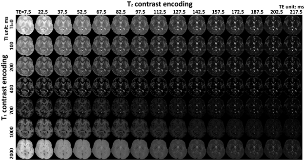
A representative single-slice 4D dataset from an in vivo human brain (the axial slice from subject 1).

FIGURE 7.

2D T₁-T₂ correlation spectra estimated from an in vivo human brain (the axial slice from subject 1). (left) Representative individual spectra plotted from different relatively “pure” voxels without substantial partial volume mixing of different components. Component 1 and component 6 are plotted from a white matter voxel, component 2 is plotted from a voxel in the putamen, component 3 is plotted from a voxel in the globus pallidus, component 4 is plotted from a voxel in gray matter, and component 5 is plotted from a voxel in the cerebral spinal fluid. In this plot, each of the spectral peaks has been numbered and color-coded (red: component 1, green: component 2, cyan: component 3, blue: component 4, yellow: component 5, and magenta: component 6). This color coding scheme was also used to depict the individual voxel locations on (middle) an anatomical reference image, although we do not mark the voxel for component 6 because it is the same as the voxel for component 1. (right) The 2D spectrum obtained by spatially-averaging the estimated 4D spectroscopic image.

FIGURE 8.

Visualization of the estimated 4D spectroscopic image from an in vivo human brain (the axial slice from subject 1). Spatially-varying 2D spectra are shown from (left) the entire image (81 × 74 voxels), (middle) a subregion of the entire image corresponding to the green box (14 × 14 voxels), and (right) an even smaller subregion corresponding to the orange box (4 × 3 voxels). In each 2D spectrum, the horizontal axis corresponds to the T₂ dimension and the vertical axis corresponds to the T₁ dimension. Each spectrum is color-coded based on the six spectral peaks and the color-coding scheme described in Fig. 7.

As can be seen in Fig. 7, we visually (subjectively) identified six spectral peaks from the estimated 4D spectroscopic image. While it may be difficult to distinguish the number of peaks that are present in the spatially-averaged spectrum, the individual peaks are actually much easier to identify when looking at the spectra from individual voxels, as can be seen in both Figs. 7 and 8. We believe that the capability to resolve six peaks is encouraging, since conventional 1D relaxometry methods generally only resolve two or three different compartments in the brain. The ability of our multidimensional correlation spectroscopic imaging approach to resolve substantially more spectral peaks with reasonable-looking spatial maps is consistent with our expectations about the superiority of high-dimensional encoding and spatial-spectral estimation relative to lower-dimensional approaches.

As can be seen in Fig. 8, we also frequently observe multiple peaks coexisting within a single voxel, and the peaks each have their own distinct spatial distributions. If we ascribe the different spectral peaks to different microstructural tissue compartments, then we can interpret this 4D spectroscopic image as demonstrating the ability to spatially map each compartment and resolve partial voluming when the compartments spatially overlap.

2D spectra obtained by spatially averaging the 4D T₁-T₂ spectroscopic image are shown for different slices and subjects in Fig. 9 (axial slices) and Supporting Information Fig. S1 (coronal slices). The number and spectral locations of the observed spectral peaks are largely the same as observed in the spectra shown in Fig. 7, demonstrating that our multidimensional correlation spectroscopic imaging approach appears to yield qualitatively similar results across a range of different subjects and slice orientations.

FIGURE 9.

Reference images (corresponding to TI = 0 and TE = 7.5 ms) and spatially-averaged 2D T₁-T₂ spectra from different axial slices of different subjects.

Spatial maps obtained by spectrally integrating the six previously-identified spectral peaks are shown in Fig. 10 (axial slices) and Supporting Information. Fig. S2 (coronal slices). We observe that these maps are also largely consistent with one another.

FIGURE 10.

Spatial maps obtained from our multidimensional correlation spectroscopic imaging approach by spectrally-integrating the six spectral peaks from axial slices of different subjects. Each map is color-coded based on the scheme from Fig. 7, and the composite image is also shown on the right.

Importantly, the spatial maps also appear to qualitatively match well with known brain anatomy: component 1 seems to correspond to a white matter (WM) compartment; component 2 seems to correspond to GM structures with relatively high myelin content, including subcortical GM, putamen, thalamus and brainstem nuclei (as seen on the wall of the fourth ventricle in subject 1 in Fig. S2) as well as cortical GM; component 3 seems to correspond to brain structures with high iron content including the globus pallidus, subthalamic nucleus and substantia nigra; component 4 is similar to component 2, but seems to represent the GM content absent any myelin-content and notably does not include the subcortical GM; component 5 seems to correspond to cerebrospinal fluid (CSF); and component 6 resembles the myelin water compartment that has been observed in previous myelin water imaging experiments^11-13,69.

It should be noted that component 3 is not observed in every slice, which we believe is reasonable because the third compartment seems localized to gray matter structures like the globus pallidus, and these structures are not present in all of the slices we acquired data from.

It should also be noted that the relaxation parameter values we estimated for component 5 (which seems to correspond to CSF) and component 6 (which resembles myelin water) do not match the parameter values for these tissue types reported in previous literature^6,8,14,70. This is somewhat expected for a variety of reasons (including simplistic modeling assumptions that do not account for magnetization transfer, slice profile effects, etc., as will be discussed in the next section), but is especially expected because the range of contrast encoding parameters we used may be insufficient to accurately estimate very quickly-relaxing tissues like myelin water or very slowly-relaxing tissues like CSF. Nevertheless, while the specific relaxation parameter values we’ve estimated are unlikely to be accurate, we are encouraged by the fact that it appears that our multidimensional correlation spectroscopic imaging approach may still be successfully resolving the spatial maps of these components, and that the resulting maps are still consistent from slice to slice and subject to subject.

For comparison, Fig. 11 shows the results obtained from the 1D T₂ relaxometry experiment. As can be seen (and consistent with previous literature^11,13), only three spectral peaks are resolved, which is substantially fewer than the number of peaks resolved by our multidimensional correlation spectroscopic imaging approach. While the spatial maps corresponding to these three peaks all appear to be anatomically reasonable, we believe that the interpretation of these maps is less straightforward than the interpretation of the spatial maps from our approach. In particular, we believe that the 1D relaxometry results are still substantially confounded by partial volume contributions, which appear to be more successfully resolved by 2D T₁-T₂ correlation spectroscopic imaging.

FIGURE 11.

Results from conventional 1D T₂ relaxation. (a) The 1D spectrum obtained by spatially-averaging the 3D spectroscopic image. (b) Representative 1D spectrum from a voxel in white matter. (c) Spatial maps obtained by spectrally-integrating the three spectral peak locations. Each map is color-coded (magenta: comp.A, green: comp.B, and yellow: comp.C), and the composite image is also shown on the right.

4 ∣. DISCUSSION

This work described our approach to multidimensional correlation spectroscopic imaging and demonstrated empirically that this approach can have better compartmental resolving power than lower-dimensional approaches. However, using higher-dimensional contrast encoding is associated with practical increases in data acquisition time. While our human brain experiments were reasonably fast, a 20 minute acquisition may still be too long for routine practical use of this technique. However, there are still plenty of opportunities to make the scan faster. For example, while our acquisition used a relatively large number (i.e., 105) of different contrast encodings, it should be noted that this number of samples was not optimized, and was chosen based on the maximum number of contrasts we could fit within a 20 minute acquisition time. We have recently presented preliminary work that uses CRLB theory to optimize experimental protocols for both 2D T₁-T₂ ⁴⁴ and 2D D-T₂ ⁷¹ correlation spectroscopic imaging. This preliminary work has demonstrated that we can obtain similar-quality results with substantially less than 105 encodings, which potentially enables substantial improvements in data acquisition time. In addition, there have been other recent constrained reconstruction approaches that have been proposed to reduce the contrast-encoding requirements of high-dimensional relaxation spectroscopy^39,40,46, as well as constrained reconstruction approaches that have been proposed to reduce the k-space sampling and averaging requirements of multi-contrast imaging^72-75. Simultaneous-multislice imaging⁷⁶ could also be used to increase the volume coverage of an acquisition without increasing the acquisition time. In addition, while we relied on an IR-MSE sequence for the results shown in this paper, our approach can also be used with other pulse sequences that may have higher efficiency such as MR fingerprinting⁷⁷, inversion recovery balanced steady-state free-precession^78,79, or a recent advanced high-dimensional contrast encoding technique⁸⁰. Multicomponent MR fingerprinting methods have also recently been described in the literature^81,82 that have similar objectives to 2D T₁-T₂ correlation spectroscopic imaging, although it does not appear that these approaches were able to resolve as many tissue compartments as our approach does. Recently, we have presented preliminary results of 2D T₁-T₂ correlation spectroscopic imaging with an MR fingerprinting acquisition with very promising results⁸³. Any of these kinds of approaches could potentially be combined to make multidimensional correlation spectroscopic imaging experiments even faster.

In this work, we used a fixed value of the regularization parameter (i.e., λ = 0.01) in all cases. This value was chosen heuristically based on the visual quality of the resulting spatial maps, and only weakly imposes spatial smoothness constraints. However, it is important to note that the choice of the regularization parameter can have an important impact on the reconstruction result. For example, Supporting Information Fig. S3 shows the results of different choices of λ. As can be seen, larger values of λ improve the apparent SNR of the resulting spatial maps, though are also associated with an apparent loss of spatial resolution (as should be expected when imposing spatial smoothness constraints). In addition, large values of the regularization parameter can be associated with substantial spectral distortions, although smaller values of λ are more benign. It is also worth noting that the unregularized reconstruction (λ = 0) is associated with substantial spatial distortions/biases, likely resulting from the ill-posedness of the inverse problem when spatial constraints are not used. While automatic “data-driven” regularization parameter selection methods have been advocated in the relaxometry literature^33,84 and are also potentially applicable to our spatial-spectral estimation approach, we believe that there may be strong benefits to characterizing the resolution characteristics of this approach using tools from the theoretical literature^65,66, such that the trade-off between noise and resolution can be understood more directly and tuned based on the needs of the particular application (e.g., as we have done in our previous work on regularized diffusion MRI⁸⁵). This promises to be an interesting topic for further research.

Although our experimental results appear to demonstrate successful decomposition of sub-voxel compartments from in vivo human subjects, some of the estimated relaxation parameters we estimated do not match closely with previous literature values. As explained previously, some of these discrepancies should be expected because our range of TEs and TIs may not be sufficient to accurately estimate very long or very short relaxation parameters. However, it is also known that quantification of relaxation parameters can be significantly affected by a variety of factors including experimental conditions, signal modeling, and optimization parameters, leading to mismatches even between different standard approaches⁸⁶. Recognizing these issues, we have focused on qualitative evaluation in real data scenarios rather than quantitative validation because of the lack of a gold standard. Nevertheless, we were able to show promising results in terms of reproducibility and consistency throughout the experiment of multiple subjects.

Although we were able to get consistently-similar and qualitatively-reasonable correlation spectroscopic imaging results, the ill-posedness of the inverse problem still means that we do not expect that our reconstructions will necessarily be the unique spectroscopic images that are consistent with the measured data. As a result, it would likely be fruitful in the future to do further exploration of the uncertainty of our solutions to the inverse problem, e.g., as might be achieved using optimization tools⁸⁷ or Monte Carlo methods^88,89.

Similarly, it is also worth noting that our application examples with the IR-MSE sequence used a relatively simple acquisition and a substantially simplified physics model that does not account for the effects of water exchange, magnetization transfer, B1 inhomogeneity, B0 inhomogeneity, slice profile effects, etc. Thus, while our current implementation appears to successfully enable separation of tissue compartments that are not easily resolved by other methods, we believe that histological validation and improving the quantitative accuracy of this kind of approach are important future objectives. (Note that it has been suggested that the standard nonnegativity constraint may be problematic for IR-MSE sequences in the presence of significant exchange⁹⁰, such that extending our approach to account for exchange may require additional modifications to our constrained estimation framework.) More accurate modeling may also enable the use of more advanced pulse sequences that may be more efficient than IR-MSE sequences but are more sensitive to nonideal acquisition physics.

Lastly, it should be noted that our estimation formulation from Eq. (8) uses a least-squares penalty to enforce consistency. The use of least-squares is appropriate under a Gaussian noise model, although the magnitude images we used in this work are more properly modeled with a Rician distribution. While the differences between Gaussian noise and Rician noise are unlikely to matter very much in high-SNR regimes, it may be valuable to investigate the use of more accurate statistical noise modeling approaches⁹¹ in future work.

5 ∣. CONCLUSION

This work presented an overview of our approach to multidimensional correlation spectroscopic imaging of exponential decays, and demonstrated a range of theoretical, simulation, and experimental results to illustrate the benefits of this approach. This approach combines high-dimensional contrast encoding with high-dimensional spatial-spectral image reconstruction to reduce the ill-posedness associated with separating multiple sub-voxel tissue compartments, enabling good results without requiring an extensive amount of pristine data. Our results demonstrate the strong potential of the method using both numerical simulations and real MRI data, including what we believe are the first in vivo human experiments of this kind. While we demonstrated 2D T₁-T₂ experiments in this work and 2D D-T₂ experiments in our previous work⁴³, we are excited by the potential of this type of approach to be used with a wider range of MR contrast parameters and/or even higher-dimensional contrast encoding.

Supplementary Material

Supp FigS1

Figure S1. Reference images (corresponding to TI =0 and TE = 7.5 ms) and spatially-averaged T₁-T₂ spectra obtained from our multidimensional correlation spectroscopic imaging approach from different coronal slices of different subjects.

Supp FigS2

Figure S2. Spatial maps obtained from our multidimensional correlation spectroscopic imaging approach by spectrally-integrating the six spectral peaks from coronal slices of different subjects. Each map is color-coded based on the scheme from Fig. 7, and the composite image is also shown on the right.

Supp FigS3

Figure S3. Numerical simulation results as a function of λ. Each subfigure shows (left) the 2D spectrum obtained by spatially-averaging the 4D spectroscopic image, (middle) spatial maps obtained by spectrally-integrating the spectral peak locations, and (right) a 2D spectrum obtained from a single representative voxel.

⁰Abbreviations:

ADMM

alternating directions method of multipliers

CPMG

Carr-Purcell-Meiboom-Gill

CRLB

Cramér-Rao lower bound

CSF

cerebrospinal fluid

GM

gray matter

ILT

inverse Laplace transform

IR-MSE

inversion-recovery multi-echo spin-echo

MRI

magnetic resonance imaging

NNLS

nonnegative least squares

PET

positron emission tomography

SNR

signal-to-noise ratio

TE

echo time

TI

inversion time

WM

white matter

APPENDIX

A ADMM BASED OPTIMIZATION ALGORITHM

In this section, we describe an ADMM based optimization algorithm to solve Eq. (8). Compared to the algorithm described in our previous work^{42,43,45,47,48} (which used vector-representations of the data and the spectroscopic image within each computation step), this work instead relies on matrix representations of the variables in Eq. (8) as described below. This difference has a practical impact, because computing each step using the matrix representation given below removes the need for for-loops and reduces computational complexity.

If we let $\mathbf{F}\in {\mathbb{R}}^{\mathrm{Q}\times \mathrm{N}}$ and $\mathrm{M}\in {\mathbb{R}}^{\mathrm{P}\times \mathrm{N}}$ represent the matrices whose ith columns respectively correspond to f_i and m_i, then the optimization problem from Eq. (8) can be more compactly represented in matrix form as

$$\widehat{\mathbf{F}}=\underset{\mathbf{F}\in {\mathbb{R}}^{Q\times N}}{\text{arg}\text{min}}\Vert \mathbf{MT}-\mathbf{KFT}{\Vert }_F^2+\lambda \Vert {\mathbf{FC}}^H{\Vert }_F^2,$$ (A1)

subject to [F]_pq ≥ 0 for ∀p = 1, … , P and ∀q = 1, … , Q. In this expression, ∥·∥_F denotes the standard Frobenius norm, $\mathbf{T}\in {\mathbb{R}}^{\mathrm{N}\times \mathrm{N}}$ is a diagonal matrix whose ith diagonal entry contains the value of t_i, C is the matrix operator that computes spatial finite differences, and (·)^H denotes the Hermitian operator (conjugate transpose). This representation is convenient for numerical optimization, but is otherwise completely equivalent to Eq. (8).

The algorithm proceeds as follows:

• Set iteration number j = 0, and initialize ${\widehat{\mathbf{F}}}^{(0)}\in {\mathbb{R}}^{\mathrm{Q}\times \mathrm{N}}$, ${\widehat{\mathbf{X}}}^{(0)}\in {\mathbb{R}}^{\mathrm{Q}\times \mathrm{N}}$, ${\widehat{\mathbf{Y}}}^{(0)}\in {\mathbb{R}}^{\mathrm{Q}\times \mathrm{N}}$, ${\widehat{\mathbf{Z}}}^{(0)}\in {\mathbb{R}}^{\mathrm{Q}\times \mathrm{N}}$, ${\mathbf{G}}^{(0)}\in {\mathbb{R}}^{\mathrm{Q}\times \mathrm{N}}$, ${\mathbf{H}}^{(0)}\in {\mathbb{R}}^{\mathrm{Q}\times \mathrm{N}}$ and ${\mathbf{R}}^{(0)}\in {\mathbb{R}}^{\mathrm{Q}\times \mathrm{N}}$ to arbitrary values. The variables X, Y, and Z are used for variable splitting, while the variables G, H, and R correspond to Lagrange multipliers. Also choose an augmented Lagrangian parameter value μ > 0 (this choice influences the convergence speed of ADMM but not the solution).

• At iteration (j + 1):

  1. For each i = 1, … , N, update the estimate of ${\widehat{\mathbf{f}}}_{\mathrm{i}}$ (i.e., the columns of $\widehat{\mathbf{F}}$) according to

     $${\widehat{\mathbf{f}}}_i^{(j+1)}=\{\begin{array}{cc}\frac{1}{3}\left({\widehat{\mathrm{x}}}_{\mathrm{i}}^{(\mathrm{j})}+{\mathrm{g}}_{\mathrm{i}}^{(\mathrm{j})}+{\widehat{\mathrm{y}}}_{\mathrm{i}}^{(\mathrm{j})}+{\mathbf{h}}_{\mathrm{i}}^{(\mathrm{j})}+{\widehat{\mathbf{z}}}_{\mathrm{i}}^{(\mathrm{j})}+{\mathbf{r}}_{\mathrm{i}}^{(\mathrm{j})}\right),\hfill & \text{if}{\mathrm{t}}_{\mathrm{i}}=1\hfill \\ \frac{1}{2}\left({\widehat{\mathrm{y}}}_{\mathrm{i}}^{(\mathrm{j})}+{\mathbf{h}}_{\mathrm{i}}^{(\mathrm{j})}+{\widehat{\mathbf{z}}}_{\mathrm{i}}^{(\mathrm{j})}+{\mathbf{r}}_{\mathrm{i}}^{(\mathrm{j})}\right),\hfill & \text{if}{\mathrm{t}}_{\mathrm{i}}=0,\hfill \end{array}\phantom{\}}$$ (A2)

     where ${\widehat{\mathrm{x}}}_{\mathrm{i}}^{(\mathrm{j})}$, ${\mathrm{g}}_{\mathrm{i}}^{(\mathrm{j})}$, ${\widehat{\mathrm{y}}}_{\mathrm{i}}^{(\mathrm{j})}$, ${\mathbf{h}}_{\mathrm{i}}^{(\mathrm{j})}$, ${\widehat{\mathbf{z}}}_{\mathrm{i}}^{(\mathrm{j})}$ and ${\mathbf{r}}_{\mathrm{i}}^{(\mathrm{j})}$ are respectively the ith columns of ${\widehat{\mathbf{X}}}^{(\mathrm{j})}$, G^(j), ${\widehat{\mathbf{Y}}}^{(\mathrm{j})}$, H^(j), ${\widehat{\mathbf{Z}}}^{(\mathrm{j})}$, and R^(j).
  2. Set

     $${\widehat{\mathbf{X}}}^{(j+1)}={\left({\mathbf{K}}^H\mathbf{K}+\mu \mathbf{I}\right)}^{-1}\left({\mathbf{K}}^H\mathbf{M}+\mu \left({\widehat{\mathbf{F}}}^{(j+1)}\mathbf{T}-{\mathbf{G}}^{(j)}\right)\right),$$ (A3)

     where I denotes the identity matrix. Note that the matrix (K^HK + μI) is small and its inverse can easily be precomputed and stored for use in every iteration.
  3. Set ${\widehat{\mathbf{Y}}}^{(\mathrm{j}+1)}={\widehat{\mathbf{F}}}^{(\mathrm{j}+1)}-{\mathbf{H}}^{(\mathrm{j})}$, but replacing any negative values with zero.
  4. Set

     $${\widehat{\mathbf{Z}}}^{(j+1)}=\mu \left({\widehat{\mathbf{F}}}^{(j+1)}-{\mathbf{R}}^{(j)}\right){\left(\mu \mathbf{I}+\lambda {\mathbf{C}}^H\mathbf{C}\right)}^{-1}.$$ (A4)

     Note that if we assume periodic boundary conditions for the spatial smoothness regularization, then the matrices I and C^HC can both be diagonalized by the discrete Fourier transform, and we can use standard Fourier methods to quickly and analytically compute the desired matrix inversion result⁶⁷.
  5. Set

     $$\begin{gathered} {\mathbf{G}}^{(\mathrm{j}+1)}={\mathbf{G}}^{(\mathrm{j})}-({\widehat{\mathbf{F}}}^{(\mathrm{j}+1)}\mathbf{T}-{\widehat{\mathbf{X}}}^{(\mathrm{j}+1)}), \\ {\mathbf{H}}^{(\mathrm{j}+1)}={\mathbf{H}}^{(\mathrm{j})}-({\widehat{\mathbf{F}}}^{(\mathrm{j}+1)}-{\widehat{\mathbf{Y}}}^{(\mathrm{j}+1)}), \\ \text{and}{\mathbf{R}}^{(\mathrm{j}+1)}={\mathbf{R}}^{(\mathrm{j})}-({\widehat{\mathbf{F}}}^{(\mathrm{j}+1)}-{\widehat{\mathbf{Z}}}^{(\mathrm{j}+1)}). \end{gathered}$$ (A5)
  6. Set j = j + 1.

• Iterate steps 1-6 until convergence.

References

- 1.Jones DK., ed.Diffusion MRI: Theory, Methods, and Applications. Oxford: Oxford University Press; . 2011. [Google Scholar]
- 2.Tournier JD, Mori S, Leemans A. Diffusion tensor imaging and beyond. Magn. Reson. Med 2011; 65(6): 1532–1556. doi: 10.1002/mrm.22924 [DOI] [PMC free article] [PubMed] [Google Scholar]
- 3.Le Bihan D, Johansen-Berg H. Diffusion MRI at 25 exploring brain tissue structure and function. NeuroImage 2012; 61: 324–341. doi: 10.1016/j.neuroimage.2011.11.006 [DOI] [PMC free article] [PubMed] [Google Scholar]
- 4.Fenrich F, Beaulieu C, Allen P. Relaxation times and microstructures. NMR Biomed. 2001; 14: 133–139. doi: 10.1002/nbm.685 [DOI] [PubMed] [Google Scholar]
- 5.Koenig S, Brown R, Spiller M, Lundbom N. Relaxometry of brain: why white matter appears bright in MRI. Magn. Reson. Med 1990; 14(3): 482–495. doi: 10.1002/mrm.1910140306 [DOI] [PubMed] [Google Scholar]
- 6.MacKay A, Laule C, Vavasour I, Bjarnason T, Kolind S, Mädler B. Insights into brain microstructure from the T2 distribution. Magn. Reson. Imag 2006; 24(4): 515–525. doi: 10.1016/j.mri.2005.12.037 [DOI] [PubMed] [Google Scholar]
- 7.Deoni SC. Quantitative relaxometry of the brain. Top. Magn. Reson. Imaging 2010; 21: 101–113. doi: 10.1097/rmr.0b013e31821e56d8 [DOI] [PMC free article] [PubMed] [Google Scholar]
- 8.Does MD. Inferring brain tissue composition and microstructure via MR relaxometry. NeuroImage 2018; 182: 136–148. doi: 10.1016/j.neuroimage.2017.12.087 [DOI] [PMC free article] [PubMed] [Google Scholar]
- 9.Kroeker RM, Henkelman RM. Analysis of biological NMR relaxation data with continuous distributions of relaxation times. J. Magn. Reson 1986; 69(2): 218–235. doi: 10.1016/0022-2364(86)90074-0 [DOI] [Google Scholar]
- 10.Whittall KP, MacKay AL. Quantitative interpretation of NMR relaxation data. J. Magn. Reson 1989; 84(1): 134–152. doi: 10.1016/0022-2364(89)90011-5 [DOI] [Google Scholar]
- 11.MacKay A, Whittall K, Adler J, Li D, Paty D, Graeb D. In vivo visualization of myelin water in brain by magnetic resonance. Magn. Reson. Med 1994; 31(6): 673–677. doi: 10.1002/mrm.1910310614 [DOI] [PubMed] [Google Scholar]
- 12.Labadie C, Lee JH, Vetek G, Springer CS. Relaxographic Imaging. J. Magn. Reson. B 1994; 105(2): 99–112. doi: 10.1006/jmrb.1994.1109 [DOI] [PubMed] [Google Scholar]
- 13.Whittall KP, MacKay AL, Graeb DA, Nugent RA, Li DKB, Paty DW. In vivo measurement of T2 distributions and water contents in normal human brain. Magn. Reson. Med 1997; 37(1): 34–43. doi: 10.1002/mrm.1910370107 [DOI] [PubMed] [Google Scholar]
- 14.Does MD, Gore JC. Compartmental study of T1 and T2 in rat brain and trigeminal nerve in vivo. Magn. Reson. Med 2002; 47(2): 274–283. doi: 10.1002/mrm.10060 [DOI] [PubMed] [Google Scholar]
- 15.Lancaster JL, Andrews T, Hardies LJ, Dodd S, Fox PT. Three-pool model of white matter. J. Magn. Reson 2003; 17(1): 1–10. doi: 10.1002/jmri.10230 [DOI] [PubMed] [Google Scholar]
- 16.Du YP, Chu R, Hwang D, et al. Fast multislice mapping of the myelin water fraction using multicompartment analysis of T2* decay at 3T: a preliminary postmortem study. Magn. Reson. Med 2007; 58(5): 865–870. doi: 10.1002/mrm.21409 [DOI] [PubMed] [Google Scholar]
- 17.Deoni SC, Rutt BK, Arun T, Pierpaoli C, Jones DK. Gleaning multicomponent T1 and T2 information from steady-state imaging data. Magn. Reson. Med 2008; 60(6): 1372–1387. doi: 10.1002/mrm.21704 [DOI] [PubMed] [Google Scholar]
- 18.Niendorf T, Dijkhuizen RM, Norris DG, v Lookeren Campagne M, Nicolay K. Biexponential diffusion attenuation in various states of brain tissue: Implications for diffusion-weighted imaging. Magn. Reson. Med 1996; 36: 847–857. doi: 10.1002/mrm.1910360607 [DOI] [PubMed] [Google Scholar]
- 19.Mulkern RV, Gudbjartsson H, Westin CF, et al. Multi-component apparent diffusion coefficients in human brain. NMR Biomed. 1999; 12: 51–62. doi: [DOI] [PubMed] [Google Scholar]
- 20.Yablonskiy DA, Bretthorst GL, Ackerman JJ. Statistical model for diffusion attenuated MR signal. Magn. Reson. Med 2003; 50(4): 664–669. doi: 10.1002/mrm.10578 [DOI] [PMC free article] [PubMed] [Google Scholar]
- 21.Assaf Y, Freidlin RZ, Rohde GK, Basser PJ. New modeling and experimental framework to characterize hindered and restricted water diffusion in brain white matter. Magn. Reson. Med 2004; 52: 965–978. doi: 10.1002/mrm.20274 [DOI] [PubMed] [Google Scholar]
- 22.Assaf Y, Blumenfeld-Katzir T, Yovel Y, Basser PJ. AxCaliber: A method for measuring axon diameter distribution from diffusion MRI. Magn. Reson. Med 2008; 59: 1347–1354. doi: 10.1002/mrm.21577 [DOI] [PMC free article] [PubMed] [Google Scholar]
- 23.Wang Y, Wang Q, Haldar JP, et al. Quantification of increased cellularity during inflammatory demyelination. Brain 2011; 134: 3590–3601. doi: 10.1093/brain/awr307 [DOI] [PMC free article] [PubMed] [Google Scholar]
- 24.Zhang H, Schneider T, Wheeler-Kingshott CA, Alexander DC. NODDI: Practical in vivo neurite orientation dispersion and density imaging of the human brain. NeuroImage 2012; 61: 1000–1016. doi: 10.1016/j.neuroimage.2012.03.072 [DOI] [PubMed] [Google Scholar]
- 25.Scherrer B, Schwartzman A, Taquet M, Sahin M, Prabhu SP, Warfield SK. Characterizing brain tissue by assessment of the distribution of anisotropic microstructural environments in diffusion-compartment imaging (DIAMOND). Magn. Reson. Med 2015; 76: 963–977. doi: 10.1002/mrm.25912 [DOI] [PMC free article] [PubMed] [Google Scholar]
- 26.Kaden E, Kelm ND, Carson RP, Does MD, Alexander DC. Multi-compartment microscopic diffusion imaging. NeuroImage 2016; 139:346–359. doi: 10.1016/j.neuroimage.2016.06.002 [DOI] [PMC free article] [PubMed] [Google Scholar]
- 27.Istratov AA, Vyvenko OF. Exponential analysis in physical phenomena. Rev. Sci. Instrum 1999; 70(2): 1233–1257. doi: 10.1063/1.1149581 [DOI] [Google Scholar]
- 28.Prony R Essai experimental et analytique: sur les lois de la dilatabilite des fluides elastiques et sur celles de la force expansive de la vapeur de l’alkool, a differentes temperatures. J L’Ecole Polytechnique 1795; 1: 24–76. [Google Scholar]
- 29.Peemoeller H, Shenoy R, Pintar M. Two-dimensional NMR time evolution correlation spectroscopy in wet lysozyme. J. Magn. Reson 1981; 45(2): 193–204. doi: 10.1016/0022-2364(81)90116-5 [DOI] [Google Scholar]
- 30.English A, Whittall K, Joy M, Henkelman R. Quantitative Two-Dimensional time Correlation Relaxometry. Magn. Reson. Med 1991; 22(2): 425–434. doi: 10.1002/mrm.1910220250 [DOI] [PubMed] [Google Scholar]
- 31.Saab G, Thompson RT, Marsh GD, Picot PA, Moran GR. Two-dimensional time correlation relaxometry of skeletal muscle in vivo at 3 Tesla. Magn. Reson. Med 2001; 46(6): 1093–1098. doi: 10.1002/mrm.1304 [DOI] [PubMed] [Google Scholar]
- 32.Hürlimann MD, Venkataramanan L. Quantitative Measurement of Two-Dimensional Distribution Functions of Diffusion and Relaxation in Grossly Inhomogeneous Fields. J. Magn. Reson 2002; 157(1): 31–42. doi: 10.1006/jmre.2002.2567 [DOI] [PubMed] [Google Scholar]
- 33.Song Y, Venkataramanan L, Hürlimann M, Flaum M, Frulla P, Straley C. T1-T2 Correlation Spectra Obtained Using a Fast Two-Dimensional Laplace Inversion. J. Magn. Reson 2002; 154(2): 261–268. doi: 10.1006/jmre.2001.2474 [DOI] [PubMed] [Google Scholar]
- 34.Callaghan PT, Godefroy S, Ryland BN. Use of the second dimension in PGSE NMR studies of porous media. Magn. Reson. Imag 2003; 21(3–4): 243–248. doi: 10.1016/S0730-725X(03)00131-0 [DOI] [PubMed] [Google Scholar]
- 35.Galvosas P, Callaghan PT. Multi-dimensional inverse Laplace spectroscopy in the NMR of porous media. C. R. Physique 2010; 11(2): 172–180. doi: 10.1016/j.crhy.2010.06.014 [DOI] [Google Scholar]
- 36.Freed DE, Hürlimann MD. One- and two-dimensional spin correlation of complex fluids and the relation to fluid composition. C. R. Physique 2010; 11: 181–191. doi: 10.1016/j.crhy.2010.06.016 [DOI] [Google Scholar]
- 37.Bernin D, Topgaard D. NMR diffusion and relaxation correlation methods: New insights in heterogeneous materials. Curr. Opin. Colloid Interface Sci 2013; 18(3): 166–172. doi: 10.1016/j.cocis.2013.03.007 [DOI] [Google Scholar]
- 38.Celik H, Bouhrara M, Reiter D, Fishbein K, Spencer R. Stabilization of the inverse Laplace transform of multiexponential decay through introduction of a second dimension. J. Magn. Reson 2013; 236: 134–139. doi: 10.1016/j.jmr.2013.07.008 [DOI] [PMC free article] [PubMed] [Google Scholar]
- 39.Bai R, Cloninger A, Czaja W, Basser PJ. Efficient 2D MRI relaxometry using compressed sensing. J. Magn. Reson 2015; 255: 88–99. doi: 10.1016/j.jmr.2015.04.002 [DOI] [PubMed] [Google Scholar]
- 40.Benjamini D, Basser PJ. Use of marginal distributions constrained optimization (MADCO) for accelerated 2D MRI relaxometry and diffusometry. J. Magn. Reson 2016; 271: 40–45. doi: 10.1016/j.jmr.2016.08.004 [DOI] [PMC free article] [PubMed] [Google Scholar]
- 41.Slator PJ, Hutter J, Palombo M, et al. Combined diffusion-relaxometry MRI to identify dysfunction in the human placenta. Magn. Reson. Med 2019; 82(1): 95–106. doi: 10.1002/mrm.27733 [DOI] [PMC free article] [PubMed] [Google Scholar]
- 42.Kim D, Kim JH, Haldar JP. Diffusion-relaxation correlation spectroscopic imaging (DR-CSI): An enhanced approach to imaging microstructure. In: Proc. Int. Soc. Magn. Reson. Med; 2016: 660. [DOI] [PMC free article] [PubMed] [Google Scholar]
- 43.Kim D, Doyle EK, Wisnowski JL, Kim JH, Haldar JP. Diffusion-relaxation correlation spectroscopic imaging: A multidimensional approach for probing microstructure. Magn. Reson. Med 2017; 78(6): 2236–2249. doi: 10.1002/mrm.26629 [DOI] [PMC free article] [PubMed] [Google Scholar]
- 44.Kim D, Wisnowski JL, Haldar JP. Improved efficiency for microstructure imaging using high-dimensional MR correlation spectroscopic imaging. In: Proc. Asilomar Conf. Sig. Sys. Comp. IEEE; 2017:1264–1268 [Google Scholar]
- 45.Kim D, Wisnowski JL, Nguyen CT, Haldar JP. Probing in vivo microstructure with T1-T2 relaxation correlation spectroscopic Imaging. In: Proc. IEEE Int. Symp. Biomed. Imag. IEEE; 2018: 675–678 [DOI] [PMC free article] [PubMed] [Google Scholar]
- 46.Benjamini D, Basser PJ. Magnetic resonance microdynamic imaging reveals distinct tissue microenvironments. NeuroImage 2017; 163: 183–196. doi: 10.1016/j.neuroimage.2017.09.033 [DOI] [PMC free article] [PubMed] [Google Scholar]
- 47.Kim D, Wisnowski JL, Haldar JP. MR correlation spectroscopic imaging of multidimensional exponential decays: probing microstructure with diffusion and relaxation. In: Proc. Wavelets and Sparsity XVII. SPIE; 2017: 103940D. [DOI] [PMC free article] [PubMed] [Google Scholar]
- 48.Kim D, Wisnowski JL, Nguyen CT, Haldar JP. Multidimensional T1 Relaxation-T2 Relaxation Correlation Spectroscopic Imaging (RR-CSI) for In Vivo Imaging of Microstructure. In: Proc. Int. Soc. Magn. Reson. Med; 2018: 783. [Google Scholar]
- 49.Lawson CL, Hanson RJ. Solving least squares problems. SIAM; . 1995. [Google Scholar]
- 50.Kay SM. Fundamentals of statistical signal processing. Prentice Hall PTR; . 1993. [Google Scholar]
- 51.Jones JA, Hodgkinson P, Barker AL, Hore PJ. Optimal sampling strategies for the measurement of spin-spin relaxation times. J. Magn. Reson. B 1996; 113: 25–34. [Google Scholar]
- 52.Cavassila S, Deval S, Huegen C, Van Ormondt D, Graveron-Demilly D. Cramér–Rao bounds: an evaluation tool for quantitation. NMR Biomed. 2001; 14(4): 278–283. doi: 10.1002/nbm.701 [DOI] [PubMed] [Google Scholar]
- 53.Ogg RJ, Kingsley PB. Optimized precision of inversion-recovery T1 measurements for constrained scan time. Magn. Reson. Med 2004; 51: 625–630. doi: 10.1002/mrm.10734 [DOI] [PubMed] [Google Scholar]
- 54.Pineda AR, Reeder SB, Wen Z, Pelc NJ. Cramér-Rao bounds for three-point decomposition of water and fat. Magn. Reson. Med 2005; 54: 625–635. doi: 10.1002/mrm.20623 [DOI] [PubMed] [Google Scholar]
- 55.Alexander DC. A general framework for experiment design in diffusion MRI and its application in measuring direct tissue-microstructure features. Magn. Reson. Med 2008; 60(2): 439–448. doi: 10.1002/mrm.21646 [DOI] [PubMed] [Google Scholar]
- 56.Zhao B, Haldar JP, Liao C, et al. Optimal Experiment Design for Magnetic Resonance Fingerprinting: Cramér-Rao Bound Meets Spin Dynamics. IEEE Trans. Med. Imag 2019; 38(3): 844–861. doi: 10.1109/TMI.2018.2873704 [DOI] [PMC free article] [PubMed] [Google Scholar]
- 57.Teixeira RPAG, Malik SJ, Hajnal JV. Joint system relaxometry (JSR) and Cramer-Rao Lower bound optimization of sequence parameters: A framework for enhanced precision of DESPOT T1 and T2 estimation. Magn. Reson. Med 2018; 79: 234–245. doi: 10.1002/mrm.26670 [DOI] [PMC free article] [PubMed] [Google Scholar]
- 58.Lin Y, Haldar JP, Li Q, Conti PS, Leahy RM. Sparsity Constrained Mixture Modeling for the Estimation of Kinetic Parameters in Dynamic PET. IEEE Trans. Med. Imag 2014; 33(1): 173–185. doi: 10.1109/TMI.2013.2283229 [DOI] [PMC free article] [PubMed] [Google Scholar]
- 59.Kumar D, Nguyen TD, Gauthier SA, Raj A. Bayesian algorithm using spatial priors for multiexponential T2 relaxometry from multiecho spin echo MRI. Magn. Reson. Med 2012; 68(5): 1536–1543. doi: 10.1002/mrm.24170 [DOI] [PubMed] [Google Scholar]
- 60.Labadie C, Lee JH, Rooney WD, et al. Myelin water mapping by spatially regularized longitudinal relaxographic imaging at high magnetic fields. Magn. Reson. Med. 2013; 71(1): 375–387. doi: 10.1002/mrm.24670 [DOI] [PubMed] [Google Scholar]
- 61.Heath MT. Scientific Computing: An Introductory Survey. McGraw-Hill; . 2002. [Google Scholar]
- 62.Matakos A, Ramani S, Fessler JA. Accelerated Edge-Preserving Image Restoration Without Boundary Artifacts. IEEE Trans. Image Process 2013; 22(5): 2019–2029. doi: 10.1109/TIP.2013.2244218 [DOI] [PMC free article] [PubMed] [Google Scholar]
- 63.Bertero M, Boccacci P . Introduction to Inverse Problems in Imaging; London: Institute of Physics Publishing; . 1998. [Google Scholar]
- 64.Haldar JP, Liang ZP. On MR experiment design with quadratic regularization. In: Proc. IEEE Int. Symp. Biomed. Imag. IEEE; 2011: 1676–1679 [Google Scholar]
- 65.Fessler JA, Rogers WL. Spatial Resolution Properties of Penalized-Likelihood Image Reconstruction: Space-Invariant Tomographs. IEEE Trans. Image Process 1996; 5: 1346–1358. doi: 10.1109/83.535846 [DOI] [PubMed] [Google Scholar]
- 66.Ahn S, Leahy RM. Analysis of Resolution and Noise Properties of Nonquadratically Regularized Image Reconstruction Methods for PET. IEEE Trans. Med. Imag 2008; 27: 413–424. doi: 10.1109/TMI.2007.911549 [DOI] [PubMed] [Google Scholar]
- 67.Afonso MV, Bioucas-Dias JM, Figueiredo MA. An augmented Lagrangian approach to the constrained optimization formulation of imaging inverse problems. IEEE Trans. Image Process 2011; 20(3): 681–695. doi: 10.1109/tip.2010.2076294 [DOI] [PubMed] [Google Scholar]
- 68.Bertero M, Boccacci P, Pike ER. On the recovery and resolution of exponential relaxation rates from experimental data: a singular-value analysis of the Laplace transform inversion in the presence of noise. Proc. R. Soc. Lond. A 1982; 383: 15–29. doi: 10.1098/rspa.1982.0117 [DOI] [Google Scholar]
- 69.Oh SH, Bilello M, Schindler M, Markowitz CE, Detre JA, Lee J. Direct visualization of short transverse relaxation time component (ViSTa). NeuroImage 2013; 83: 485–492. doi: 10.1016/j.neuroimage.2013.06.047 [DOI] [PMC free article] [PubMed] [Google Scholar]
- 70.Does MD, Beaulieu C, Allen PS, Snyder RE. Multi-component T1 relaxation and magnetisation transfer in peripheral nerve. Magn. Reson. Med 1998; 16(9): 1033–1041. doi: 10.1016/S0730-725X(98)00139-8 [DOI] [PubMed] [Google Scholar]
- 71.Kim D, Haldar JP. Faster Diffusion-relaxation correlation spectroscopic imaging (DR-CSI) using Optimized Experiment Design. In: Proc. Int. Soc. Magn. Reson. Med; 2017: 176. [DOI] [PMC free article] [PubMed] [Google Scholar]
- 72.Haldar JP, Liang ZP. Joint reconstruction of noisy high-resolution MR image sequences. In: Proc. IEEE Int. Symp. Biomed. Imag. IEEE; 2008: 752–755 [Google Scholar]
- 73.Gong E, Huang F, Ying K, Wu W, Wang S, Yuan C. PROMISE: Parallel-imaging and compressed-sensing reconstruction of multicontrast imaging using sharable information. Magn. Reson. Med 2015; 73(2): 523–535. doi: 10.1002/mrm.25625 [DOI] [PubMed] [Google Scholar]
- 74.Zhao B, Lu W, Hitchens TK, Lam F, Ho C, Liang ZP. Accelerated MR parameter mapping with low-rank and sparsity constraints. Magn. Reson. Med 2015; 74(2): 489–498. doi: 10.1002/mrm.25421 [DOI] [PMC free article] [PubMed] [Google Scholar]
- 75.Bilgic B, Kim TH, Liao C, et al. Improving parallel imaging by jointly reconstructing multi-contrast data. Magn. Reson. Med 2018; 80(2): 619–632. doi: 10.1002/mrm.27076 [DOI] [PMC free article] [PubMed] [Google Scholar]
- 76.Barth M, Breuer F, Koopmans PJ, Norris DG, Poser BA. Simultaneous multislice (SMS) imaging techniques. Magn. Reson. Med 2016; 75(1): 63–81. doi: 10.1002/mrm.25897 [DOI] [PMC free article] [PubMed] [Google Scholar]
- 77.Ma D, Gulani V, Seiberlich N, et al. Magnetic resonance fingerprinting. Nature 2013; 495(7440): 187–192. doi: 10.1038/nature11971 [DOI] [PMC free article] [PubMed] [Google Scholar]
- 78.Schmitt P, Griswold MA, Jakob PM, et al. Inversion recovery TrueFISP: Quantification ofT1,T2, and spin density. Magn. Reson. Med 2004; 51(4): 661–667. doi: 10.1002/mrm.20058 [DOI] [PubMed] [Google Scholar]
- 79.Pfister J, Breuer FA, Jakob PM, Blaimer M. Fast multi-component T1 and T2 correlation measurements using steady-state free precession. In: Proc. Int. Soc. Magn. Reson. Med; 2018: 220. [Google Scholar]
- 80.Hutter J, Slator PJ, Christiaens D, et al. Integrated and efficient diffusion-relaxometry using ZEBRA. Scientific Reports 2018; 8(1): 15138. doi: 10.1038/s41598-018-33463-2 [DOI] [PMC free article] [PubMed] [Google Scholar]
- 81.McGivney D, Deshmane A, Jiang Y, et al. Bayesian estimation of multicomponent relaxation parameters in magnetic resonance fingerprinting. Magn. Reson. Med 2018; 80(1): 159–170. doi: 10.1002/mrm.27017 [DOI] [PMC free article] [PubMed] [Google Scholar]
- 82.Tang S, Fernandez-Granda C, Lannuzel S, et al. Multicompartment magnetic resonance fingerprinting. Inverse Problems 2018; 34(9): 094005. doi: 10.1088/1361-6420/aad1c3 [DOI] [PMC free article] [PubMed] [Google Scholar]
- 83.Kim D, Bo Z, Wald LL, Haldar JP. Multidimensional T1 Relaxation -T2 Relaxation Correlation Spectroscopic Imaging with a Magnetic Resonance Fingerprinting Acquisition. In: Proc. Int. Soc. Magn. Reson. Med; 2019: In Press. [Google Scholar]
- 84.Zou YL,Xie RH, Arad A. Numerical estimation of the choice of the regularization parameter for NMR T2 inversion. Pet.Sci 2016; 13: 237–246. [Google Scholar]
- 85.Haldar JP, Wedeen VJ, Nezamzadeh M, et al. Improved diffusion imaging through SNR-enhancing joint reconstruction. Magn. Reson. Med 2013; 69: 277–289. [DOI] [PMC free article] [PubMed] [Google Scholar]
- 86.Stikov N, Boudreau M, Levesque IR, Tardif CL, Barral JK, Pike GB. On the accuracy of T1 mapping: Searching for common ground. Magn. Reson. Med 2014; 73(2): 514–522. doi: 10.1002/mrm.25135 [DOI] [PubMed] [Google Scholar]
- 87.Parker RL, Song YQ. Assigning uncertainties in the inversion of NMR relaxation data. J. Magn. Reson 2005; 174: 314–324. doi: 10.1016/j.jmr.2005.03.002 [DOI] [PubMed] [Google Scholar]
- 88.Prange M, Song YQ. Quantifying uncertainty in NMR spectra using Monte Carlo inversion. J. Magn. Reson 2009; 196(1): 54–60. doi: 10.1016/j.jmr.2008.10.008 [DOI] [PubMed] [Google Scholar]
- 89.Prange M, Song YQ. Understanding NMR spectral uncertainty. J. Magn. Reson 2010; 204(1): 118–123. doi: 10.1016/j.jmr.2010.02.010 [DOI] [PubMed] [Google Scholar]
- 90.Dortch RD, Horch RA, Does MD. Development, simulation, and validation of NMR relaxation-based exchange measurements. J. Chem. Phys 2009; 131(16): 164502. doi: 10.1063/1.3245866 [DOI] [PMC free article] [PubMed] [Google Scholar]
- 91.Varadarajan D, Haldar JP. A majorize-minimize framework for Rician and non-central chi MR images. IEEE Trans. Med. Imag 2015; 34: 2191–2202. doi: 10.1109/TMI.2015.2427157 [DOI] [PMC free article] [PubMed] [Google Scholar]
Associated Data
This section collects any data citations, data availability statements, or supplementary materials included in this article.
Supplementary Materials