Artificial Intelligence Applied to Osteoporosis: A Performance Comparison of Machine Learning Algorithms in Predicting Fragility Fractures From MRI Data

Abstract

Background:

A current challenge in osteoporosis is identifying patients at risk of bone fracture.

Purpose:

To identify the machine learning classifiers that predict best osteoporotic bone fractures and, from the data, to highlight the imaging features and the anatomical regions that contribute most to prediction performance.

Study Type:

Prospective (cross-sectional) case–control study.

Population:

Thirty-two women with prior fragility bone fractures, of mean age = 61.6 and body mass index (BMI) = 22.7 kg/m², and 60 women without fractures, of mean age = 62.3 and BMI = 21.4 kg/m².

Field Strength/Sequence: 3D FLASH at 3T.

Assessment:

Quantitative MRI outcomes by software algorithms. Mechanical and topological microstructural parameters of the trabecular bone were calculated for five femoral regions, and added to the vector of features together with bone mineral density measurement, fracture risk assessment tool (FRAX) score, and personal characteristics such as age, weight, and height. We fitted 15 classifiers using 200 randomized cross-validation datasets.

Statistical Tests:

Data: Kolmogorov–Smirnov test for normality. Model Performance: sensitivity, specificity, precision, accuracy, F1-test, receiver operating characteristic curve (ROC). Two-sided t-test, with P < 0.05 for statistical significance.

Results:

The top three performing classifiers are RUS-boosted trees (in particular, performing best with head data, F1 = 0.64 ± 0.03), the logistic regression and the linear discriminant (both best with trochanteric datasets, F1 = 0.65 ± 0.03 and F1 = 0.67 ± 0.03, respectively). A permutation of these classifiers comprised the best three per-formers for four out of five anatomical datasets. After averaging across all the anatomical datasets, the score for the best performer, the boosted trees, was F1 = 0.63 ± 0.03 for All-features dataset, F1 = 0.52 ± 0.05 for the no-MRI dataset, and F1 = 0.48 ± 0.06 for the no-FRAX dataset.

Data Conclusion:

Of many classifiers, the RUS-boosted trees, the logistic regression, and the linear discriminant are best for predicting osteoporotic fracture. Both MRI and FRAX independently add value in identifying osteoporotic fractures. The femoral head, greater trochanter, and inter-trochanter anatomical regions within the proximal femur yielded better F1-scores for the best three classifiers.

OSTEOPOROSIS is a debilitating disease that can lead to a higher incidence of bone fracture. In diagnosing a patient with osteoporosis, their bone mineral density (BMD) is compared with that of a reference group: a gender-and ethnicity-matched healthy, young adult population.¹ This method, however, leads to many individuals not receiving clinically prudent treatment. There are a few reasons for this. BMD is measured via dual-energy x-ray absorptiometry (DXA), a 2D projection imaging technique. The nature of this test often results in the underestimation or overestimation of the BMD.² For example, in patients with small bones the BMD is underestimated, and in patients with overlying vascular calcifications or osteophytes the BMD is inflated. As a result of this inaccuracy, the majority of patients who suffer osteoporotic fractures do not meet the DXA criterion for osteoporosis.³

In recent years, however, magnetic resonance imaging (MRI) has brought added diagnostic power to many diseases, including musculoskeletal ones. The parameters it provides can be sensitive to microstructural changes in the bone, which in turn may be useful for predicting fracture risk.³ Parallel to developments in the field of MRI, machine learning (ML) has made inroads into many domains of science. The results obtained are of a statistical nature, dependent on the data used, the models employed, and the metrics of performance. Previous studies have looked at the methods for comparing ML algorithms. A study by Demšar,⁵ which followed the proceedings of the International Conference on Machine Learning from 1999 to 2003, found a surprisingly high over-reliance on classification accuracy alone, reiterating the need for more performance measures. Sokolova et al.⁶ stress as important properties of a classifier the ability to not only correctly identify classes but also to discriminate between the label classes.

Medical diagnostic measurements have recently been analyzed with ML to extract new and unexpected risk factors and disease patterns. A study by Madelin et al.⁷ employed many ML classifiers, and used sodium MRI data from cartilage, for diagnosing osteoarthritis. Using both standard and adjusted accuracy, as well as sensitivity and specificity, the study identified the linear models as best performers, over neural networks, K-nearest neighbors (KNN), or quadratic-kernel support vector machine (SVM).

In studies of osteoporosis, ML has already been applied to predict hip fractures. Kruse et al.⁸ used clustering, an unsupervised ML method, to extract nine layers of different osteoporotic fracture risk from data on 10,775 subjects. A later study by the same group⁹ used twenty-four different models to identify hip fractures from a Danish cohort of 5439 women and men. In both of these reports, the parameters include DXA measurements, age, and even dental or medication expenses (but not MRI data).

In this study we used MRI data for osteoporosis to compare 15 ML classifiers. We also investigated the impact that MRI and fracture risk assessment (FRAX) metric have in identifying osteoporotic fractures and, in particular, which of the five proximal femoral regions provided better classification.

Materials and Methods

The next sections describe the data acquisition and preprocessing (first three subsections), followed by an explanation of the feature selection process and the resulting datasets. Then we describe the classifiers, and the metrics we use to compare them.

Cohort Characteristics

The study was approved by the Institutional Review Board and was performed in compliance with HIPAA. All subjects provided informed written consent. The only criteria for inclusion is postmenopausal women, older than 18 years of age, and with no upper limit; none of the participants had any known comorbidities. The dataset consisted of 92 women who presented for examination at our hospital, of whom 32 had prior fragility fractures (age = 61.6 ± 8.4, body mass index [BMI] = 22.7 ± 3.1) and 60 who did not (age = 62.3 ± 7.8, BMI = 21.4 ± 2.8). Of those with fractures, there were 20 subjects with one fracture, 9 subjects with two fractures, and 3 subjects with more than two fractures. The type of fractures were: wrist (n = 7), spine (n = 2), humerus (n = 1), hip (n = 3), humerus +hip (n = 1), sacrum (n = 1), sacrum+wrist (n = 1), sacrum+hip (n = 1), and other (n = 15).

Imaging Data

The dataset’s 92 subjects presented for high-resolution 3T MRI (Magneton Prisma, Siemens, Erlangen, Germany) examination of the proximal femur (D-FLASH, repetition time [TR] = 37 msec, echo time [TE] = 4.92 msec, flip angle = 25, bandwidth = 130 Hz/pixel, field of view [FOV] = 100 mm, matrix = 512 × 3 × 512, voxel = 0.234 × 0.234 × 1.5 mm³, GRAPPA parallel imaging factor = 2, scan-time = 15 min). Mechanical and microstructural MRI measures of bone quality were obtained via finite element and topological analysis, as described by Wehrli et al.¹⁰ and Saha et al.,¹¹ in five 10 × 10 × 10 mm³ volumes of interest within the femoral head (hereafter referred to as “head”), femoral neck (“neck”), Ward’s triangle (“ward”), greater trochanter (“troch”), and intertrochanteric region (“inter-troch”).

Complete Feature Set

From the MRI data we extracted parameters that are expected to be altered by osteoporosis and, therefore, reflect deterioration in the microarchitecture of the trabecular bone compartment. Our criterion for labeling any one data vector as osteoporotic was the presence of bone fractures; this dichotomous separation disregards the actual number of fractures.

The mechanical parameters for subregional analysis are described in Wehrli et al.,¹⁰ whereas the topological parameters are described in Saha et al.¹¹ as “characterizing the local topology of each bone voxel after skeletonization of the binary bone images.” Here, each voxel of trabecular bone network is labeled as either surface, curve or junction structure. The topology of the network is characterized by the surface-to-curve ratio and erosion index. (For clarity, in this study, we reserve the term parameters to measurements from MRI.)

In summary, the MRI parameter types are:

• mechanical: elastic moduli X/Y/Z, and shear moduli G11/G22/G33;

• physical: the mean/SD of bone volume/density/thickness;

• topological: the edges/interiors/junctions of the curve/surface;

• statistical: the normalized topological features of the above.

In addition to the above 32 MRI parameters, the primary dataset also includes these measurements: height, weight, BMI, age, two FRAX (hip and overall), and two DXA metrics (spine and femoral neck t-score).

Feature Selection

We apply the principal component analysis (PCA) method^12,13 on the primary dataset to construct a reduced feature set. Each of the many principal components is a linear combination of the original features, with every feature being weighted differently. The weights are the inverse of the variance of each original feature. The components are conventionally ordered by the amount of variance that each explains. So, the first component explains the most, the second aims to capture as much variance as possible that could not be captured by the first, and so on (the components are also linearly independent, or orthogonal; that is, no one component can be reconstructed from a combination of the rest). Choosing the number of these components, ie, the dimension of the feature space is not so straightforward, and there are many “rules of thumb”, generally based on the amount of variance explained. For comparison, here we try three low/medium/maximum levels of components from a total of 55 features in the original dataset: the minimum required to explain 95% of the variance in the data (the results show this to be 5), another level close to the middle (we chose 30), and the maximum (55).

Datasets

The primary and the three PCA-feature datasets are four of the six datasets we will use. The remaining two datasets are derived from the primary dataset: one excludes the FRAX features (No-FRAX), whereas the other (No-MRI) excludes the MRI features. The purpose for doing this is to, first, evaluate the benefit that each of FRAX and MRI bring to the fracture prediction; and second, to compare FRAX’s diagnostic power with that of the imaging parameters.

ML Classifiers

To each dataset we fit 15 classifiers, roughly belonging to the groups below. Here we give a brief description of each class of classifiers, as taken from Michie et al¹⁴ and Friedman et al,¹⁵ from which a more detailed description of these classifiers can be found.

• linear models (the logistic regression and the linear discriminant). The logistic regression and the linear discriminant are both linear classifiers. Although closely related, the logistic regression is less dependent on the data distribution—the linear discriminant prefers normally distributed data—when separating the sample space (with lines in 2D, planes in 3D, or hyperplanes in higher dimensions). The shape of the clusters of the separated data classes dictates the location and direction of these dividing planes.

• SVM (of linear, quadratic, and cubic kernels). SVMs attempt to improve linear model fitting by searching for the maximum-margin hyperplane separating the two classes. Additionally, for cases where the classes overlap, thus requiring nonlinear boundaries, SVMs allow the use of (here, quadratic or cubic) kernels that transform the original sample space into a higher-dimensional space where a linear boundary can be drawn.

• trees (simple, medium, and complex tree). A decision tree is a tree-like chart, root-to-leaf, where at each node a test (dependent on previous steps/nodes) is carried out, and the branch carries the result (ultimately to the leaf ). This can be seen as a recursive partitioning of the sample space. In our case, a “simple” tree has four maximum splits (there-fore, few leaves to distinguish between the classes), a medium tree has at most 20 splits, whereas a complex tree has 100 splits at most (more leaves to make finer distinctions between the classes). The maximum number of splits is typically referred to as the maximum depth of a tree. Other than being relatively easy to understand and follow, another advantage of trees is that they are fairly immune to variable transformations, the variables of low relevance, and outliers. Because of these advantages, the decision trees have become the most popular tool in data mining.

• KNN (fine, weighted) The idea for a KNN partitioning is that each given datum is most likely to be near to observations from its own proper class population. So, one looks at, say, the five nearest observations from all previously recorded subjects, and classifies the observation according to the most frequent class among its neighbors. In the “fine” KNN classifier, the number of neighbors is set to 1, i.e., a fine distinction between the classes; whereas in the “weighted” KNN classifier, the number of neighbors is set to 10, and the classes are distinguishable using a distance metric.

• ensemble (for KNN, linear discriminant, RUS-boosted, and bagged trees). The ensemble learning combines the strengths of a collection of simpler base models. In tree bagging, a committee of trees each cast a vote for the predicted class. In boosting, the committee of weak learners evolves over time, and the members cast a weighted vote.

Using the MatLab Statistics Toolbox (MathWorks, Natick, MA), we fit the classifiers via the commands given in the Appendix (Supplementary Information). In fitting the classifiers we settle for the standard fitting routines as provided by MatLab, which can hopefully be utilized by the clinician with minimal effort. Notwithstanding this caveat, we do consider some variations (such as the kernel degree in SVM, or lasso regularization with logistic regression) which can potentially alter the classifier’s performance.

Statistics

We examined the pairwise linear correlation between the features through Pearson’s correlation coefficient r; this is the product of the standard deviations of the two feature pairs, divided by their covariance. Whenever two populations are compared, we use a two-sided t-test. We use a P value threshold of 0.05 for statistical significance. When comparing two data vectors we ensure, through the Kolmogorov–Smirnov test, that they follow a normal distribution.

The metrics for comparing the classifiers are:

$$\text{sensitivity}=\frac{\text{tp}}{\text{tp}+\text{fn}}$$

$$\text{specificity}=\frac{\mathrm{tn}}{\mathrm{tn}+\text{fp}}$$

$$\text{precision}=\frac{\mathrm{tp}}{\mathrm{tp}+\text{fp}}$$

$$\text{accuracy}=\frac{\text{tp}+\text{fp}}{\text{tp}+\text{fp}+\text{tn}+\text{fn}}$$

$$\text{F}1=2*\frac{{\text{sensitivity}}^{*}\text{specificity}}{\text{sensitivity}+\text{specificity}}$$

$$\text{AUC=}\text{area}\text{under}\text{the}\text{ROC}\text{curve}$$

Here, tp stands for the true positives, tn for true negatives, fp for false positives, and fn for false negatives. For the AUC calculation we use the implementation of Will Dwinnell, using the Ling et al¹⁶ algorithm. All metrics range from 0 to 1.

The k-fold crossvalidation (CV) is a natural model selection technique that penalizes complexity and helps identify the classifier most robust to noise. In our 23-fold CV, the classifier is trained on 22/23rds of the randomly sampled dataset, and then is tested on the remaining 1/23rd. The aggregate predicted fracture vector is then compared with the original, and the above six performance metrics are then calculated. This is repeated 200 times, each time using a random starting seed point for partitioning the dataset into folds. We report the metrics’ mean and standard deviation across these 200 CV iterations.

Results

Figure 1 shows representative proximal femur MR images from a patient with fragility fracture and a control subject.

FIGURE 1:

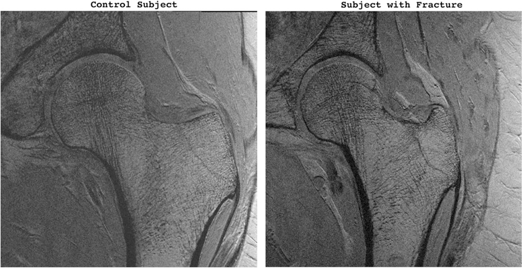
Representative coronal MR images of proximal femur from a control subject (left panel) and a subject with osteoporotic fracture (right panel).

In Fig. 2, the positional variance diagram for the features’ pairwise correlations maps the interdependence of the features. Although the mechanical features (first six from the top left) have strong interdependence, r = 0.99 ± 0.004, they are independent from the rest, r = 0.06 ± 0.03. The other imaging features (ie, the remainder, bar age, height, weight, FRAX, and DXA) show some correlation, r = 0.53 ± 0.29.

FIGURE 2:

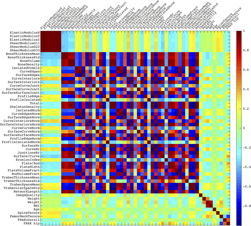
A positional variance diagram for the pairwise linear correlations between the features. The color scale indicates the correlation from 1 (strongly, positively correlated), through 0 (not correlated), to –1 (strongly, negatively correlated).

Figure 3 explores the redundancy in the feature set (as suggested by Fig. 1). PCA analysis on the representative head data reveals that the first three components explain 90% of the data variance, while five explain over 95%. The next subplot shows the weight of each original head data feature on the first three PCA components. We see that bone thick-ness, topological features (such as ratios of surface-to-curve or plate-to-rod), and non-imaging data (e.g., weight and age) have the largest impact. Similar feature families appear over other anatomical regions, as shown in the third subplot.

FIGURE 3:

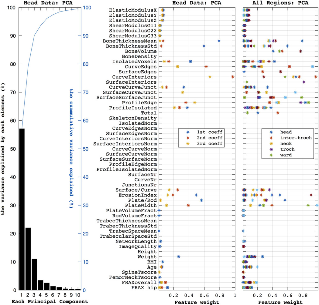
The first subplot (on the left) shows the components produced by the PCA when using the head data. The first three components explain ~95% of the variance (as shown by the blue line). The second plot shows how much each feature weighs in producing the three most important principal components (accounting for ~95% of the variance) for the head dataset. Similarly, the third subplot summarizes the PCA weights over the five anatomical regions, as color marked in the legend.

Figure 4 shows the classifiers’ performance in identifying unseen labels, averaged over all anatomical datasets (head, troch, etc.). In ordering the classifiers, the plots use the F1-score of ALL features dataset. In the ALL features ranking, the top three classifiers are the RUS-boosted trees, the logistic regression, and the linear discriminant, with F1 = 0.63 ± 0.04, 0.62 ± 0.05, 0.60 ± 0.07, respectively; KNN variations come last, with F1 = 0.21 ± 0.06 for the weighted-KNN classifier. When compared with the dataset with ALL features, PCA with five components performs worse in the better 12 of the 15 classifiers. PCA with 30 components performs better in 12 classifiers with mixed performance; in particular, there is no statistically significant difference in good classifiers such as cubic SVM (fourth in the ranking) or the linear discriminant (ranked third) when compared with the ALL data. The same number of PCA components as ALL (55) makes no statistically significant improvement in two out of three best classifiers after comparison with ALL data results (these are denoted with arrows in the figure). Because of this picture of classifiers performance on PCA, in the next plots we will only use the original data with ALL features.

FIGURE 4:

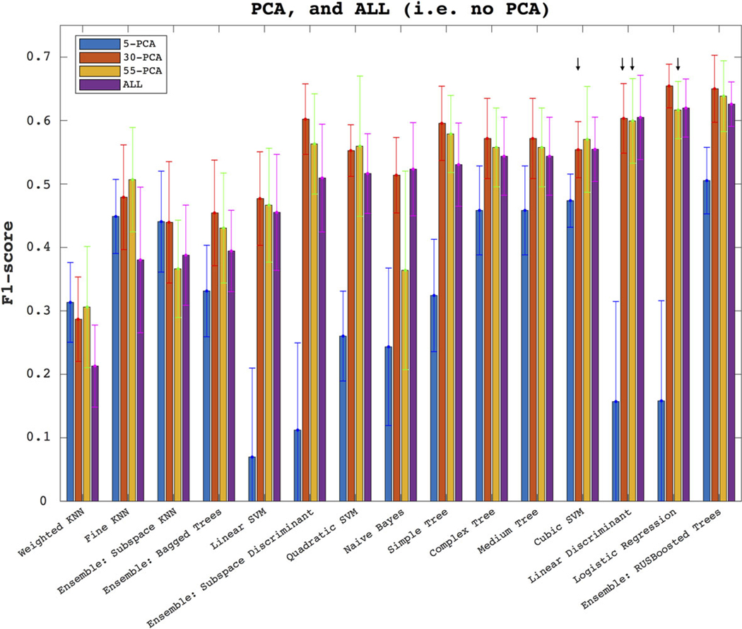
The plots show how the models perform through the F1-score, when using selected PCA components (first three bars on each classifier, as denoted in the legend), and the complete set of features (denoted in the legend as ALL, plotted in each classifier’s last bar). The results are averaged over the five anatomical subregions. In the legend, 5-PCA denotes a PCA with only five components, etc. The error bars denote the standard deviation around the mean across 200 random-seed initializations of the 23-fold CV. The arrows denote no statistically significant difference between the pointed population and that of ALL.

The six subplots of Fig. 5 show the classifiers performance in the six metrics: sensitivity, specificity, accuracy, precision, AUC, and F1-score. Each subplot shows the classifier ranking for three datasets: marked red is the complete ALL features dataset (as also observed in Fig. 4), marked green is the complete dataset excluding the MRI features, and marked blue is the complete dataset without FRAX. Through almost all classifiers, and certainly all the top 10, and across all metrics, adding MRI and FRAX improves the performance. For example, for the RUS-boosted trees, the F1-score for ALL, no-MRI, and no-FRAX were respectively 0.63 ± 0.03, 0.52 ± 0.05, 0.48 ± 0.06. The sensitivity performance of classifiers shows an opposite trend to that specificity. The precision metric offers some models, such as linear SVM (0.68 ± 0.07), which is clearly better than the rest (eg, boosted trees’ precision, at 0.49 ± 0.04).

FIGURE 5:

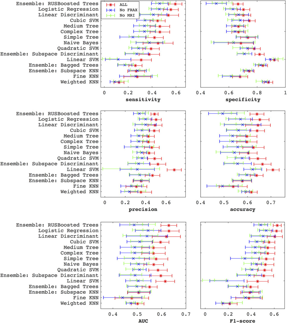
The plots show how the classifiers perform via the sensitivity, specificity, precision, accuracy, AUC, and F1-score metrics, after averaging over the five anatomical subregions. The classifiers are ordered by the F1-score ranking. Clearly, both MRI and FRAX improve performance. The trend of sensitivity across the classifiers runs in the opposite direction to that specificity.

Beyond the standard logistic regression, which ranks as one of the best three classifiers, we also tried lasso (not shown in the figures), which provides L1-regularization to the fitting.¹⁷ While lasso improved the specificity (from 0.71–0.83) and accuracy (from 0.66–0.71), it penalized sensitivity (down from 0.60–0.50), resulting in a slight F1-score change (from 0.65–0.67). Additionally, the fitting of the regularization parameter lambda is very sensitive to variations in the data.

In Fig. 6 we show the F1-score performance through the five anatomical regions. We see similar patterns of classifier performance as in Fig. 4. The previously identified three classifiers remain the best for three regions: the head, the inter-troch, and troch. The linear discriminant (F1 = 0.67 ± 0.03) is best in the troch dataset, as is the logistic regression (F1 = 0.65 ± 0.03); boosted trees are best with head data (F1 = 0.64 ± 0.03). It is clear that, for the best three classifiers, the neck data provides the worst results (coming 5^th/5^th/5^th), followed by ward (4^th/4^th/2^nd), and the better regions are head (3^rd/3^rd/2^nd), inter-troch (2^nd/2^nd/3^rd) and troch (1^st/1^st/3^rd); however, there is no statistically significant difference between head, troch, and inter-troch when using the logistic regression.

FIGURE 6:

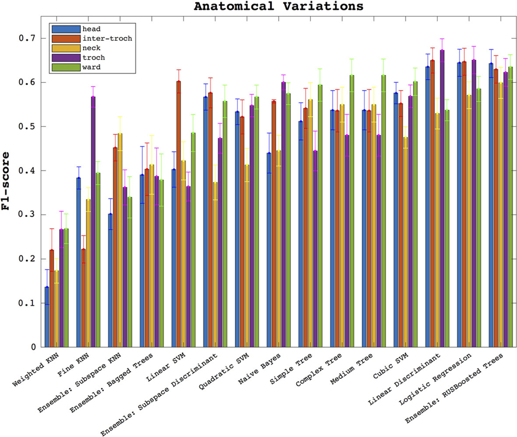
Here we show the F1-score performance across the datasets of all five anatomical regions.

Discussion

A current challenge in osteoporosis is identifying patients with a higher propensity for bone fracture. In this initial study, we applied ML techniques to bone microstructural MRI data collected at our hospital. Our first finding is that the combination of MRI plus FRAX data improved the ability of ML models to predict patients’ osteoporotic fracture status compared with MRI or FRAX data alone. The second finding is that linear classifiers and boosted trees perform best in predicting fracture. The third finding is that certain anatomical regions within the proximal femur (head, inter-troch, and troch) yielded better F1-scores (than ward or neck).

The finding that the combination of MRI plus FRAX improves the predictive abilities of ML models, rather than either MRI or FRAX, suggests that MRI-derived microstructural measures could potentially have value for clinicians in terms of more accurately diagnosing and therefore more accurately treating patients at risk for fracture. If this were validated in a prospective fracture incidence study, it would improve patient outcomes and potentially save healthcare costs by preventing future osteoporotic fractures, as suggested in a previous cost-effectiveness study.¹⁸ Furthermore, the finding that certain proximal femur datasets yielded better F1-scores suggests that more informative indices about patients’ bone quality/health may be obtained within these proximal femur subregions; again, this result needs to be confirmed in the future, ideally in prospective longitudinal studies.

Differently from other ML studies on osteoporosis, our study uses MRI data. The evidence of correlation between the features, shown in the first two figures, pertains to the linear correlation only, and other nonlinear dependencies were not accounted for. This is also the case for the PCA analysis. Even though PCA with half the original number of features did almost as well or slightly better, we made a choice to show the remainder of the analysis use ALL of the original features instead. One reason is that the principal components have generally little clinical interpretability. In our case, given the limited data, it would have been impractical trying to go beyond the linear dependence. Without strong evidence of linear dependence between the features, here we argue that obtaining PCA components that can capture the majority of the data variance comes at the risk of diminished sensitivity, and therefore may not necessarily translate into correct labeling. Nevertheless, the top three classifiers remained the same with both PCA and ALL features. In the future, parameters such as blood and genetic tests may add more predictive ability; and with this greater quantity of data, the choice of methodology for feature selection and classification will remain important.

Our study showed that simple classifiers, such as logistic regression and linear discriminant, remain good models for datasets of this size, alongside boosted trees and SVM. Considering that different classifiers may be more appropriate in different applications, this is consistent with the classifier comparison study by Madelin et al,⁷ which also finds that linear models are better predictors over Naive Bayes, quadratic-kernel SVM, or KNN. Sokolova et al⁶ suggest that Naive Bayes does better on positive examples (middle-rank performer in our ranking), while SVM does better on negative examples (linear SVM was top classifier for precision, whereas the cubic kernel SVM’s F1-score was fourth best).

In this study, among the six metrics, we used F1-score as our primary metric, capturing both sensitivity and specificity, and because we judged it better than others. As mentioned in the introduction, most current literature reports the accuracy.⁵ However, by definition this statistic assumes a balanced dataset of fracture versus control labels (otherwise good classifiers would be biased towards predicting the majority class, usually the negatives). Some researchers prefer ROC metrics; Ling et al¹⁶ argue that it is a better discriminator than accuracy. But the interpretation of results is not so straightforward as, for example, the ROC weighs sensitivity and specificity equally at all threshold levels.¹⁹ This is certainly not the case for every disease. Some studies report sensitivity and specificity, and a minority report Youden’s index, being sensitivity+specificity-1.²⁰ Although this may be an improvement, it does not discriminate against scenarios where both sensitivity and specificity are at mediocre or extreme levels, as some of our worst performing classifiers’ results demonstrate.

Notwithstanding these results, our study has some limitations. The first comes from the rather limited size of the cohort (92 subjects, of which 30 had fractures). One obvious consequence is that the data are not naturally balanced; the fracture and no-fracture cohorts are not in equal proportion, which in turn will affect the CV sampling, potentially biasing certain statistics. On the subject of balance, we also mention here that our dataset consists of a purely female cohort, which is the predominantly osteoporosis-affected gender. Further studies may be necessary to examine the generalizability of the results.

Another inevitable limitation arises from the multitude of fitting routines that are possible for each of the classifiers. In the interest of repeatability, we compared off-the-shelf models with default settings and minimal optimization. With an ever-increasing model complexity, the classifiers run the risk of being overtuned to the training dataset and its noise (although one could argue that CV already does penalize for overfitting). We also have the clinician in mind, who may wish to utilize a quick and standard ML method as an additional tool for assessing fracture risk in a patient with osteoporosis. Each model’s performance can of course be optimized for any given metric (eg, sensitivity or accuracy), sampling method (eg, bootstrapping or CV), and data (specific to a geographical location, anatomical region, age, gender, etc.).

In conclusion, we found that ML classifiers such as the logistic regression, the linear discriminant, or boosted trees provide the best balance of sensitivity and specificity for predicting osteoporotic fracture, and that both MRI and FRAX independently add value in identifying osteoporotic fractures through ML.

References

- 1.Kanis JA. Assessment of fracture risk and its application to screening for postmenopausal osteoporosis: synopsis of a WHO report. Osteoporos Int 1994;4:368–381. [DOI] [PubMed] [Google Scholar]
- 2.Bolotin HH. DXA in vivo BMD methodology: an erroneous and misleading research and clinical gauge of bone mineral status, bone fragility, and bone remodelling. Bone 2007;41:138–154. [DOI] [PubMed] [Google Scholar]
- 3.Siris ES, Chen Y-T, Abbott TA, et al. Bone mineral density thresholds for pharmacological intervention to prevent fractures. Arch Intern Med 2004; 164:1108–1112. [DOI] [PubMed] [Google Scholar]
- 4.Wehrli FW. Structural and functional assessment of trabecular and cortical bone by micro magnetic resonance imaging. J Magn Reson Imaging 2007;25:390–409. [DOI] [PubMed] [Google Scholar]
- 5.Demšar J. Statistical comparisons of classifiers over multiple data sets. J Mach Learn Res 2006;7:1–30. [Google Scholar]
- 6.Sokolova M, Japkowicz N, Szpakowicz S. Beyond accuracy, F-score and ROC: a family of discriminant measures for performance evaluation. In: Australian Conference on Artificial Intelligence, 2006;4304:1015–1021. [Google Scholar]
- 7.Madelin G, Poidevin F, Makrymallis A, Regatte RR. Classification of sodium MRI data of cartilage using machine learning. Magn Reson Med 2015;74:1435–1448. [DOI] [PMC free article] [PubMed] [Google Scholar]
- 8.Kruse C, Eiken P, Vestergaard P. Clinical fracture risk evaluated by hierarchical agglomerative clustering. Osteoporos Int 2017;28:819–832. [DOI] [PubMed] [Google Scholar]
- 9.Kruse C, Eiken P, Vestergaard P. Machine learning principles can improve hip fracture prediction. Calcif Tissue Int 2017;100:348–360. [DOI] [PubMed] [Google Scholar]
- 10.Wehrli FW, Rajapakse CS, Magland JF, Snyder PJ. Mechanical implications of estrogen supplementation in early postmenopausal women. J Bone Miner Res 2010;25:1406–1414. [DOI] [PMC free article] [PubMed] [Google Scholar]
- 11.Saha PK, Gomberg BR, Wehrli FW. Three-dimensional digital topological characterization of cancellous bone architecture. Int J Imaging Syst Technol 2000;11:81–90. [Google Scholar]
- 12.Pearson K. LIII. On lines and planes of closest fit to systems of points in space. London, Edinburgh, and Dublin Philosophical Magazine and Journal of Science 1901;2:559–572. [Google Scholar]
- 13.Jolliffe IT. Choosing a subset of principal components or variables Principal Component Analysis. New York, NY: Springer, 1986; 92–114. [Google Scholar]
- 14.Michie D, Spiegelhalter DJ, Taylor CC, eds. Machine learning, neural and statistical classification. Hertfordshire, UK: Ellis Horwood; 1994. [Google Scholar]
- 15.Friedman J, Hastie T, Tibshirani R. The elements of statistical learning. Vol. 1 New York: Springer Series in Statistics; 2001. [Google Scholar]
- 16.Ling CX, Huang J, Zhang H, et al. AUC: a statistically consistent and more discriminating measure than accuracy. IJCAI 2003;3:519–524. [Google Scholar]
- 17.Tibshirani R. Regression shrinkage and selection via the lasso. J R Stat Soc B Methodol 1996:267–288. [Google Scholar]
- 18.Agten CA, Ramme AJ, Kang S, Honig S, Chang G. Cost-effectiveness of virtual bone strength testing in osteoporosis screening programs for postmenopausal women in the United States. Radiology 2017;285: 506–517. [DOI] [PMC free article] [PubMed] [Google Scholar]
- 19.Halligan S, Altman DG, Mallett S. Disadvantages of using the area under the receiver operating characteristic curve to assess imaging tests: a discussion and proposal for an alternative approach. Eur Radiol 2015;25: 932–939. [DOI] [PMC free article] [PubMed] [Google Scholar]
- 20.Fehr D, Veeraraghavan H, Wibmer A, et al. Automatic classification of prostate cancer Gleason scores from multiparametric magnetic resonance images. Proc Natl Acad Sci U S A 2015;112:E6265–E6273. [DOI] [PMC free article] [PubMed] [Google Scholar]
Associated Data
This section collects any data citations, data availability statements, or supplementary materials included in this article.