Evaluating and Differentiating a Polynomial Using a Pseudo-witness Set

Abstract

Polynomials which arise via elimination can be difficult to compute explicitly. By using a pseudo-witness set, we develop an algorithm to explicitly compute the restriction of a polynomial to a given line. The resulting polynomial can then be used to evaluate the original polynomial and directional derivatives along the line at any point on the given line. Several examples are used to demonstrate this new algorithm including examples of computing the critical points of the discriminant locus for parameterized polynomial systems.

Introduction

Parameterized polynomial systems arise in various applications in science and engineering, such as in computer vision [15, 17, 22], kinematics [14, 23], and chemistry [1, 19]. Often in these applications, real solutions are desired. The complement of the discriminant locus associated with the parameterized polynomial system consists of cells where the number of real solutions is constant. Elimination methods (e.g., see [8, Chap. 3]) theoretically provide an approach to explicitly compute a defining equation for the discriminant locus. If the discriminant locus is a curve or surface, there are several numerical methods that can be used to plot it, e.g., [6, 7, 18]. When the explicit expression is difficult to compute, this paper develops a numerical algebraic geometric approach based on pseudo-witness sets [13] for both evaluating implicitly defined polynomials and directional derivatives. In particular, the approach yields an explicit univariate polynomial equal to the defining equation restricted to a line which can then be evaluated or differentiated as needed. When the parameterized system and line have rational coefficients, the resulting univariate polynomial also has rational coefficients which can be computed exactly from the numerical data [2].

One application of this new approach is to compute the critical points of the discriminant polynomial which are outside of the discriminant locus without explicitly computing the discriminant. This set of critical points contains at least one point in each compact cell in the complement of the discriminant locus [10] which can be useful for determining the possible number of real solutions as well as the real monodromy structure [11].

The remainder of the paper is as follows. Section 2 describes the approach based on using pseudo-witness sets. Section 3 presents an algorithm for performing the computations with some illustrative examples. Section 4 provides two examples of computing critical points.

Implicit Representation of a Polynomial

In numerical algebraic geometry, e.g., see [4, 21], a witness point set for a hypersurface consists of the intersection points of with a line . Suppose that f(x) is a given polynomial and is the hypersurface defined by the vanishing of f. Then, the witness point set for corresponds with the roots of the univariate polynomial obtained by restricting f to the line . Since every univariate polynomial is defined up to scale by its roots, one can recover by computing its roots along with knowing for some value T which is not a root of . The following is an illustration of this basic setup.

Example 1

Consider the polynomial with corresponding hypersurface and the line defined parametrically by:

Therefore, one can explicitly compute

1

For and , one has

2

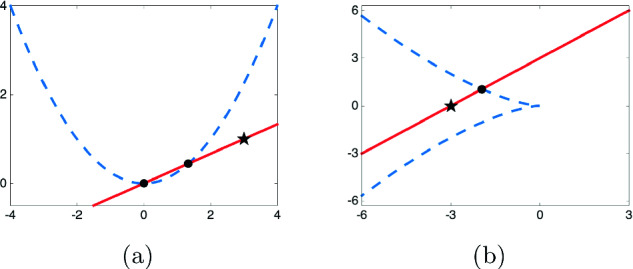
Hence, for some constant s which can be computed from, say, requiring where , i.e., . Therefore, one has recovered in (1) from with as illustrated in Fig. 1(a).

Fig. 1.

A visual representation of the pseudo-witness set for defined by with a linear slice, , that is (a) generic, (b) special with one root of multiplicity one, and (c) tangent. The black dots represent the roots and the black stars represent T selected for scale.

The remainder of this section extends this idea using pseudo-witness sets when f is a polynomial over that is not known explicitly, but the corresponding hypersurface  arises as the closure of a projection of an algebraic set. For simplicity of presentation, assume that is a polynomial system and that V is a pure d-dimensional subset of . Let such that . Note that one has . A pseudo-witness set [13] for , say , is a numerical algebraic geometric data structure that permits computations on without knowing the defining polynomial f for . The last two items are a linear space and a finite set . In particular, where is a codimension general linear space so that has codimension d. Hence, is a witness point set for with respect to . With this setup, the local multiplicity of each point in can be easily computed via [5, Prop. 6] (see also [9, pg. 158]). Thus, parameterizing by t and denoting as the corresponding points in with multiplicity , respectively, yields

3

as shown in the following.

Theorem 1

The univariate polynomial describing f along the line is correctly described by (3).

Proof

The assumption on T is that , i.e., . Hence, is a nonzero polynomial which has finitely many roots, namely with multiplicity , respectively. Thus, with . Since the roots define the univariate polynomial up to scale, the leading coefficient is used to achieve the desired value at T and thus everywhere along .

The following illustrates a pseudo-witness set and Theorem 1.

Example 2

Consider the hypersurface from Example 1 under the assumption that we are given where and with

Since and , we have with

where and are as in Example 1 with . Hence, as in (2). Therefore, with and , (3) simplifies to in (1).

The only assumption on the line is that so that one can find T such that . Of course, one can check if by a pseudo-witness set membership test [12] in which case one would simply have . Thus,  is not necessarily assumed to intersect transversely, so the number of roots and multiplicities can vary for different choices of . Nonetheless, Theorem 1 applies as is illustrated in the following two examples.

Example 3

Reconsider Example 2 with being the vertical line parametrized by

as shown in Fig. 1(b). One has and with and . For scale, consider with . Thus, (3) yields

Example 4

Reconsider Example 2 with being the horizontal line parametrized by

as shown in Fig. 1(c). One has and with and . For scale, consider with . Thus, (3) yields

Clearly, once the univariate polynomial in (3) is computed explicitly, one can easily determine the value of f at any point along via evaluation. Moreover, if is parameterized by , then is equal to the directional derivative of f with respect to v at , denoted .

Example 5

For in Example 3 and Example 4, one has and , respectively. Hence, the corresponding directional derivatives are simply partial derivatives of with respect to y and x, respectively. From Example 3, one obtains while Example 4 yields and .

Algorithm

Theorem 1 immediately justifies Algorithm 1 for explicitly computing a polynomial restricted to a line. The following two examples exemplify this algorithm applied to the discriminant locus.

Example 6

Consider the discriminant locus for . Hence, where and with

For the line parameterized by

with , one has . The other input for Algorithm 1 is, say, with to set the scale. This setup is illustrated in Fig. 2(a).

Fig. 2.

Pseudo-witness set for the discriminant locus of (a) the quadratic and (b) the cubic .

The pseudo-witness set yields and with . The corresponding scale factor is

so that Algorithm 1 returns .

Of course, one can easily compute that the discriminant of g satisfying is with .

Example 7

Consider the discriminant locus for . Hence, where and with

For the line parameterized by

with , one has, rounded to 4 decimal places with ,

The other input for Algorithm 1 is, say, with for scale. This setup is illustrated in Fig. 2(b).

The pseudo-witness set yields , , and with . The corresponding scale factor is so that .

As in Example 6, one can easily compute that the discriminant of g satisfying is with as above.

Computing Critical Points

When the line is fixed, Algorithm 1 computes the restriction of a polynomial f to . The following presents two examples of combining this idea with homotopy continuation to compute critical points of f, namely . The set of real solutions to with contains at least one point in each compact cell of [10]. The website dx.doi.org/10.7274/r0-0mc0-gt33 contains the necessary files to perform these computations using Bertini [3].

Lemniscate

This first example demonstrates the approach given which defines a lemniscate, but utilizes a pseudo-witness set for the computation. The aim is to compute all real solutions of and . For genericity, replace with the equivalent condition that the directional derivatives of f in both the and directions, namely and , vanish for general and . We used , and in our computation.

Since one is setting directional derivatives equal to zero, the scale factor is irrelevant and can be simply set to 1. We first compute a witness set for each of the cubic curves defined by and where each of them are expressed in terms of univariate roots following Sect. 2. Then, we simply intersect these two cubic curves using a diagonal homotopy [20] that tracks  paths. There are 3 finite endpoints corresponding with the 3 solutions of , all of which are real and shown in Fig. 3(a). Two of these have with one in each of the two compact cells of .

Fig. 3.

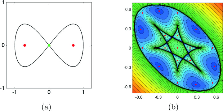
(a) The lemniscate with 2 critical points satisfying (red) and the other satisfying (green), and (b) the discriminant locus (black) for the 3-oscillator Kuramoto model with contour plot and 19 real critical points (red) in the complement. (Color figure online)

Kuramoto Model

The Kuramoto model [16] is a mathematical model of an oscillating system to describe synchronization. After a standard conversion to polynomials, the discriminant locus for the steady states of the 3-oscillator Kuramoto model is modeled by where and  with

4

Letting f be a defining polynomial for , the aim is to compute the real solutions of with using a pseudo-witness set for . As in Sect. 4.1, we replace with the equivalent condition that two general directional derivatives vanish. In this case, the vanishing of a general directional derivative of f yields a degree 11 curve, so a diagonal homotopy [20] to intersect the vanishing of two directional derivatives tracks paths. This yields 103 finite solutions consisting of 37 that satisfy which can be verified using a membership test via a pseudo-witness set for [12]. Sorting through these 37 yields 19 real critical points with . Figure 3(b) plots the real part of along with these 19 real critical points on a contour plot of f showing that at least one is contained in each compact cell of .

References

- 1.Al-Khateeb, A.N.: One-dimensional slow invariant manifolds for spatially homogeneous reactive systems. J. Chem. Phys. 131 (2009) [DOI] [PubMed]
- 2.Bates DJ, Hauenstein JD, McCoy TM, Peterson C, Sommese AJ. Recovering exact results from inexact numerical data in algebraic geometry. Exp. Math. 2013;22(1):38–50. doi: 10.1080/10586458.2013.737640. [DOI] [Google Scholar]
- 3.Bates, D.J., Hauenstein, J.D., Sommese, A.J., Wampler, C.W.: Bertini: software for numerical algebraic geometry. bertini.nd.edu
- 4.Bates, D.J., Hauenstein, J.D., Sommese, A.J., Wampler, C.W.: Numerically solving polynomial systems with Bertini. SIAM (2013)
- 5.Bernardi A, Daleo NS, Hauenstein JD, Mourrain B. Tensor decomposition and homotopy continuation. Differ. Geom. Appl. 2017;55:78–105. doi: 10.1016/j.difgeo.2017.07.009. [DOI] [Google Scholar]
- 6.Besana GM, Di Rocco S, Hauenstein JD, Sommese AJ, Wampler CW. Cell decomposition of almost smooth real algebraic surfaces. Numer. Algor. 2013;63:645–678. doi: 10.1007/s11075-012-9646-y. [DOI] [Google Scholar]
- 7.Chen C, Wu W. A numerical method for computing border curves of bi-parametric real polynomial systems and applications. In: Gerdt VP, Koepf W, Seiler WM, Vorozhtsov EV, editors. Computer Algebra in Scientific Computing; Cham: Springer; 2016. pp. 156–171. [Google Scholar]
- 8.Cox DA, Little J, O’Shea D. Ideals, Varieties, and Algorithms. 4. Cham: Springer; 2015. [Google Scholar]
- 9.Fischer G. Complex Analytic Geometry. Heidelberg: Springer; 1976. [Google Scholar]
- 10.Harris, K., Hauenstein, J.D., Szanto, A.: Smooth points on semi-algebraic sets. arXiv:2002.04707 (2020)
- 11.Hauenstein JD, Regan MH. Real monodromy action. Appl. Math. Comput. 2020;373:124983. [Google Scholar]
- 12.Hauenstein JD, Sommese AJ. Membership tests for images of algebraic sets by linear projections. Appl. Math. Comput. 2013;219(12):6809–6818. [Google Scholar]
- 13.Hauenstein JD, Sommese AJ. Witness sets of projections. Appl. Math. Comput. 2010;217(7):3349–3354. [Google Scholar]
- 14.Hauenstein JD, Wampler CW, Pfurner M. Synthesis of three-revolute spatial chains for body guidance. Mech. Mach. Theory. 2017;110:61–72. doi: 10.1016/j.mechmachtheory.2016.12.008. [DOI] [Google Scholar]
- 15.Irschara, A., Zach, C., Frahm, J.M., Bischof, H.: From structure-from-motion point clouds to fast location recognition. In: CVPR, pp. 2599–2606. IEEE (2009)
- 16.Kuramoto Y. Self-entrainment of a population of coupled non-linear oscillators. In: Araki H, editor. International Symposium on Mathematical Problems in Theoretical Physics. Heidelberg: Springer; 1975. pp. 420–422. [Google Scholar]
- 17.Leibe, B., Cornelis, N., Cornelis, K., Van Gool, L.: Dynamic 3D scene analysis from a moving vehicle. In: CVPR, pp. 1–8. IEEE (2007)
- 18.Lu Y, Bates DJ, Sommese AJ, Wampler CW. Finding all real points of a complex curve. Contemp. Math. 2007;448:183–205. doi: 10.1090/conm/448/08665. [DOI] [Google Scholar]
- 19.Morgan AP. Solving Polynomial Systems Using Continuation for Engineering and Scientific Problems. Englewood Cliffs: Prentice-Hall; 1987. [Google Scholar]
- 20.Sommese AJ, Verschelde J, Wampler CW. Solving polynomial systems equation by equation. In: Dickenstein A, Schreyer FO, Sommese AJ, editors. Algorithms in Algebraic Geometry. New York: Springer; 2008. pp. 133–152. [Google Scholar]
- 21.Sommese AJ, Wampler CW. The Numerical Solution of Systems of Polynomials Arising in Engineering and Science. Hackensack: World Scientific; 2005. [Google Scholar]
- 22.Snavely, N., Seitz, S.M., Szeliski, R.: Photo tourism: exploring photo collections in 3D. In: ACM SIGGRAPH, pp. 835–846 (2006)
- 23.Wampler CW, Sommese AJ. Numerical algebraic geometry and algebraic kinematics. Acta Numerica. 2011;20:469–567. doi: 10.1017/S0962492911000067. [DOI] [Google Scholar]