

Abstract
We present the Julia interface
 to polymake, a software for research in polyhedral geometry. We describe the technical design and how the integration into Julia makes it possible to combine polymake with state-of-the-art numerical software.
Keywords: Polymake, Julia
Introduction
polymake is an open source software system for computing with a wide range of objects from polyhedral geometry and related areas [4]. This includes convex polytopes and polyhedral fans as well as matroids, finite permutation groups, ideals in polynomial rings and tropical varieties. The user is interfacing the polymake library through Perl language.
In this note we provide a brief overview of a new interface
 , which allows the use of polymake in Julia [1]. Julia is a high-level, dynamic programming language. Distinctive aspects of Julia’s design include a type system with parametric polymorphism and multiple dispatch as its core programming paradigm. The package
 can be installed, without any preparations, using the build-in package manager that comes with Julia. The source code is available at https://github.com/oscar-system/Polymake.jl.
Functionality
In polymake the objects that a user encounters can be roughly divided into the following three classes
big objects (e.g., cones, polytopes, simplicial complexes),
small objects (e.g., matrices, polynomials, tropical numbers),
user functions.
Broadly speaking, big objects correspond to mathematical concepts with well defined semantics. These can be queried, accumulate information (e.g., a polytope defined by a set of points can “learn” its hyperplane representation), and are constructed usually in Perl. Big objects implement methods, i.e., functions which operate on, and perform computations specific to the corresponding object. Small objects correspond to types or data structures which are implemented in
 . Standalone user functions are exposed to the user via the Perl interpreter.
These entities are mapped to Julia in the following way:
big objects are exposed as opaque Perl objects that can be queried for their properties (they are only computed when queried for the first time),
small objects are wrapped through an intermediate
 layer between Julia and
 generated by
 ,
,methods and user functions are mapped to Julia functions, in the case of methods, the parent object being the first argument.
A unique feature of
 is based on the affinity of Julia to C and
 programming languages. As Julia provides the possibility to call functions from dynamic libraries directly, one can call any function from the polymake library as long as the function symbol is exported. In polymake, due to extensive use of templates in the
 library, the precise definition of a function needs to be often explicitly instantiated. Such instantiaton can be easily added to the

 wrapper. An example of such functionality is
![]()
a function, which directly taps into the polymake framework for linear programming. It is worth pointing that the signature of the exposed solve_LP will accept any instances of Julias
 or
or
 (where appropriate) in the paradigm of generic programming.
Technical Contribution
The
 interface is based on
 1, a Julia package which aims to provide a seamless interoperability between
 and Julia. The interface is separated into two parts: a
 wrapper library and a Julia package. The former,
 , a dynamic library, wraps the data structures (small types) in a Julia-compatible way and exposes functions from the callable
 polymake library. It is then loaded through
 where the Julia part of the package generates functions accessible from Julia.
The installation of
 is performed through Julia’s package manager with the help of
 infrastructure. Thanks to this infrastructure it is not necessary for the user to perform any preparations except for installing Julia itself. All dependencies of
 (including the polymake library, the Perl interpreter and supplementary libraries) are installed in a binary form. The complete installation of
 should take no longer than 5 minutes on modern hardware
Due to extensive use of metaprogramming, relatively little code was necessary to make most of the functionality of polymake available in Julia: as of version 0.4.1
 consists of about 1200 lines of
 code and 1600 lines of Julia code. In particular, only the small objects need to be manually wrapped, while functions, constructors for big objects and their methods are generated automatically from the information provided by polymake itself. This automatic code generation takes place during precompilation which is done only once during the installation. Loading
 brings the familiar polymake welcome banner.

The latest version of
 is 0.4.1 which is compatible with at Julia 1.3 and newer. The latest polymake version is available in
 within two weeks of release (currently polymake 4.0).
Big Objects
All big objects are constructed by direct calls to their constructors, e.g. ![]() constructs a rational polytope from (homogeneous) coordinates of points given row-wise. We attach the polymake docstring to the structure such that the documentation is readily available in Julia.
constructs a rational polytope from (homogeneous) coordinates of points given row-wise. We attach the polymake docstring to the structure such that the documentation is readily available in Julia.

Template parameters can also be passed to big objects, e.g., to construct a polytope with floating point precision it is sufficient to call
![]()
A caveat is that all parameters must be valid Julia objects.2 The properties of big objects are accessible through the
 syntax which mirrors the
 syntax in polymake. Note that some properties of big objects in polymake are indeed methods with no arguments and therefore in Julia they are only available as such.
Small objects
The list of small objects available in
 includes basic types such as arbitrary size integers (subtypes
 , rationals (subtypes
 , vectors and matrices (subtypes of
 ), and many more. These data types can be converted to appropriate Julia types, but are also subtypes of the corresponding Julia abstract types (as indicated above). This allows to use
 types in generic methods, which is the paradigm of Julia programming.
As already mentioned, these small objects need to be manually wrapped in the
 part of
 . In particular, all possible combinations of such types, e.g., an array of sets of rationals, need to be explicitly wrapped. Note that polymake is able to generate dynamically any combination of small objects. Thus, we cannot guarantee that all small objects a user will encounter is covered. However, the small objects available in
 are sufficient for the most common use cases.
Functions
A function in
 calling polymake may return either a big or a small object, and the generic return type (PropertyValue, a container opaque to Julia) is transparently converted to one of the known (small) data types3. If the data type of the returned function value is not known to
 , the conversion fails and an instance of PropertyValue is returned. It can be either passed back as an argument to a
 function, or converted to a known type using the
 macro.

All user functions from polymake are available in modules corresponding to their applications, e.g.
 functions from the application topaz can be called as
 in Julia. Moreover polymake docstrings for functions are available in Julia to allow for easy help4:

Function Arguments. Functions in
 accept the following as their arguments: simple data types (bools, machine integers, floats), wrapped native types, or objects returned by polymake (e.g.,
 , or PropertyValue). Due to the easy extendability of methods in Julia, a foreign type could be passed seamlessly to
 function if an appropriate
 method, which return one of the above types, is defined:
![]()
Polymake.jl also wraps the extensive visualization methods of polymake which can be used to produce images and animations of geometric objects. These include the interactive visualizations using three.js. Due to the convenient extendability of Julia, the visualization also integrates seamlessly with Jupyter notebooks.
Example
This section demonstrates the interface of
 on a concrete example. An advantage of the package is that it allows effortless combination of computations in polyhedral geometry with e.g., state-of-the-art numerical software. Here we combine
 with
with
 [3], a Julia package for numerically solving systems of polynomial equations. In particular, we test a theoretical result from Soprunova and Sottile [8] on non-trivial lower bounds for the number of real solutions to sparse polynomial systems.
The results show how we can construct a sparse polynomial system that has a non-trivial lower bound on the number of real solutions starting from an integral point configuration. We start with the 10 lattice points  of the scaled two-dimensional simplex
  and look at the regular triangulation
  induced by the lifting
  .
.

The triangulation  is very special in that it is foldable (or “balanced”), i.e., the dual graph is bipartite. This means that the triangles can be colored, say, black and white such that no two triangles of the same color share an edge. See Fig. 1 for an illustration. The signature
 of a balanced triangulation of a polygon is the absolute value of the difference of the number of black triangles and the number of the white triangles whose normalized volume is odd. The vertices of a foldable triangulation can be colored by
  colors [6] (such that vertices of the same color do not share an edge), where d is the dimension. Here
  , so 3 colors suffice. We can check both properties with polymake.
Fig. 1.
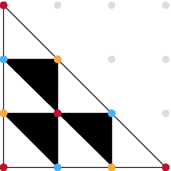
Foldable subdivision of  .
.

Now, a Wroński polynomial
 has the lifted lattice points as exponents, and only one non-zero coefficient
  per color class of vertices of the triangulation
 |
A Wroński system consists of d Wroński polynomials with respect to the same lattice points A and lifting  such that for general
  it has precisely
  distinct complex solutions, which is the highest possible number by Kushnirenko’s Theorem [7].
Soprunova and Sottile showed that a Wroński system has at least  distinct real solutions if two conditions are satisfied. First, a certain double cover of the real toric variety associated with A must be orientable. This is the case here. Second, the Wroński center ideal, a zero-dimensional ideal in coordinates
  and s depending on
  , has no real roots with s coordinate between 0 and 1. Let us verify this condition using
 . Luckily for us, polymake already has an implementation of the Wroński center ideal. However, we have to convert the ideal returned by
 to a polynomial system which
 understands. This can be accomplished with a simple routine.

Since we are only interested in solutions in the algebraic torus  we can use polyhedral homotopy [5] to efficiently compute the solutions.

Out of the 54 complex roots only two solutions are real. Strictly speaking, this is here only checked heuristically by looking at the size of the imaginary parts. However, a certified version can be obtained by using
 [2]. By closer inspection, we see that no solution has the s-coordinate in (0, 1).

Therefore, the Wroński system with respect to A and  for
for  has at least
  real solutions. Let us verify this on an example.

Finally, we can use the
 package to visualize the real solutions of the Wroński system W (Fig. 2).
Fig. 2.
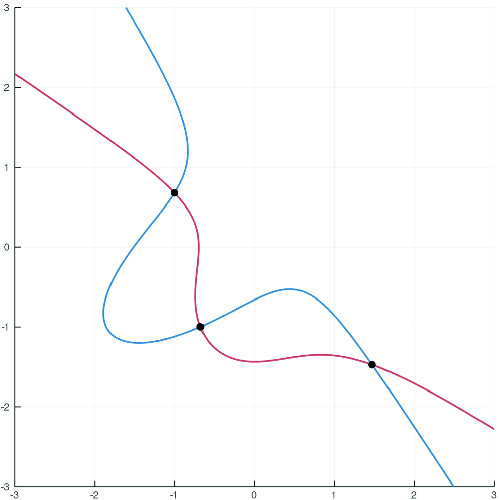
Visualization of the Wroński system W and its 3 solutions.

Acknowledgements
We would like to express our thanks to Alexej Jordan and Sebastian Gutsche for all their help during the development of
 .
.
Footnotes
Available at https://github.com/JuliaInterop/CxxWrap.jl.
For advanced use (when this is not the case) we provide the @pm macro.
This conversion can be deactivated by passing PropertyValue type as the first argument to function/method call.
The documentation currently uses the Perl syntax.
M. Kaluba—The author was supported by the National Science Center, Poland grant 2017/26/D/ST1/00103. This research is carried out in the framework of the DFG funded Cluster of Excellence EXC 2046 MATH+: The Berlin Mathematics Research Center within the Emerging Fields area.
S. Timme—The author was supported by the Deutsche Forschungsgemeinschaft (German Research Foundation) Graduiertenkolleg Facets of Complexity (GRK 2434).
Contributor Information
Anna Maria Bigatti, Email: bigatti@dima.unige.it.
Jacques Carette, Email: carette@mcmaster.ca.
James H. Davenport, Email: j.h.davenport@bath.ac.uk
Michael Joswig, Email: joswig@math.tu-berlin.de.
Timo de Wolff, Email: t.de-wolff@tu-braunschweig.de.
Sascha Timme, Email: timme@math.tu-berlin.de.
References
- 1.Bezanson J, Edelman A, Karpinski S, Shah VB. Julia: a fresh approach to numerical computing. SIAM Rev. 2017;59(1):65–98. doi: 10.1137/141000671. [DOI] [Google Scholar]
- 2.Hauenstein JD, Sottile F. Algorithm 921: alphaCertified: certifying solutions to polynomial systems. ACM Trans. Math. Softw. (TOMS) 2012;38(4):1–20. doi: 10.1145/2331130.2331136. [DOI] [Google Scholar]
- 3.Breiding, P., Timme, S.: HomotopyContinuation.jl: a package for homotopy continuation in Julia. In: International Congress on Mathematical Software, pp. 458–465. Springer (2018)
- 4.Gawrilow E, Joswig M. polymake: a framework for analyzing convex polytopes. Polytopes–combinatorics and computation (Oberwolfach, 1997) DMV Sem. 2000;29:43–73. [Google Scholar]
- 5.Huber B, Sturmfels B. A polyhedral method for solving sparse polynomial systems. Math. Comput. 1995;64(212):1541–1555. doi: 10.1090/S0025-5718-1995-1297471-4. [DOI] [Google Scholar]
- 6.Joswig M. Projectivities in simplicial complexes and colorings of simple polytopes. Math. Z. 2002;240:243–259. doi: 10.1007/s002090100381. [DOI] [Google Scholar]
- 7.Kushnirenko AG. A Newton polyhedron and the number of solutions of a system of k equations in k unknowns. Usp. Math. Nauk. 1975;30(1975):266–267. [Google Scholar]
- 8.Soprunova E, Sottile F. Lower bounds for real solutions to sparse polynomial systems. Adv. Math. 2006;204:116–151. doi: 10.1016/j.aim.2005.05.016. [DOI] [Google Scholar]