Abstract
In this article, we propose the Susceptible-Unidentified infected-Confirmed (SUC) epidemic model for estimating the unidentified infected population for coronavirus disease 2019 (COVID-19) in China. The unidentified infected population means the infected but not identified people. They are not yet hospitalized and still can spread the disease to the susceptible. To estimate the unidentified infected population, we find the optimal model parameters which best fit the confirmed case data in the least-squares sense. Here, we use the time series data of the confirmed cases in China reported by World Health Organization. In addition, we perform the practical identifiability analysis of the proposed model using the Monte Carlo simulation. The proposed model is simple but potentially useful in estimating the unidentified infected population to monitor the effectiveness of interventions and to prepare the quantity of protective masks or COVID-19 diagnostic kit to supply, hospital beds, medical staffs, and so on. Therefore, to control the spread of the infectious disease, it is essential to estimate the number of the unidentified infected population. The proposed SUC model can be used as a basic building block mathematical equation for estimating unidentified infected population.
Keywords: Epidemic model, Least-squares fitting, COVID-19
1. Introduction
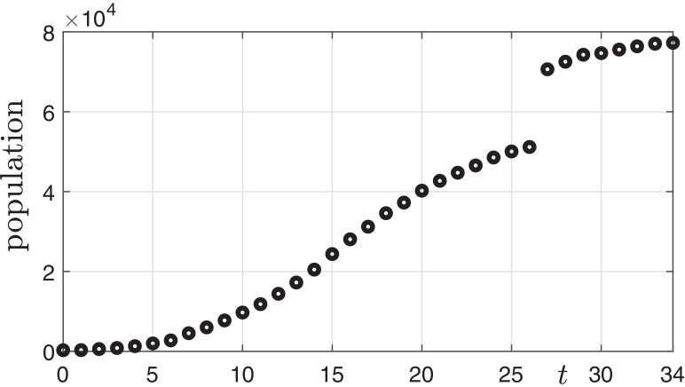
The coronavirus disease 2019 (COVID-19) was first identified in Wuhan, China in December 2019 [1]. The numbers of the COVID-19 confirmed cases in China from 21 January to 24 February 2020 are shown in Fig. 1 . The data was reported by World Health Organization (WHO) as of 24 February 2020 [2].
Fig. 1.
Epidemic curve of COVID-19 confirmed cases from 21 January to 24 February 2020.
Currently, there are many active research about COVID-19: In [3], the authors presented the impact of reduced travel volume to and from China on the transmission dynamics of COVID-19 outside China. Roosa et al. [4] used phenomenological models to generate short-term forecasts of cumulative reported cases in Guangdong and Zhejiang, China. In [5], the authors presented the distribution of incubation periods estimated for travellers from Wuhan with confirmed COVID-19 infection in the early outbreak phase. Hellewell et al. [6] developed a stochastic transmission model to assess the effects of isolation and contact tracing.
In this paper, we propose the Susceptible-Unidentified infected-Confirmed (SUC) epidemic model for estimating the unidentified infected population for COVID-19 in China. In the Susceptible-Unidentified infected-Confirmed (SUC) epidemic model, the total population N is divided into the susceptible S(t), unidentified infected U(t), and confirmed C(t) individuals at time t:
S(t) = susceptible; individuals who are not infected but are capable of contracting the disease and becoming infective.
U(t) = unidentified infected; individuals who are infected but have not yet been confirmed, and therefore are not isolated.
C(t) = confirmed; individuals who have been infected and confirmed, including all cases of recovery or death (i.e., the removed).
Based on the assumptions above, the equations governing the SUC model are as follows:
| (1) |
| (2) |
| (3) |
Here, N is the total population and thus we assume that is always satisfied. We disregard changes in population due to birth and death irrelevant to the infectious disease. Therefore, Eq. (3) can be replaced by Eq. (4).
| (4) |
The transmission is expressed by the standard incidence where β represents the disease transmission rate [7]. We assume the unidentified infected U(t) are not yet hospitalized and still can spread the disease to the susceptible S(t).
The parameter γ is the probability of cases where disease is confirmed among the unidentified infected. We assume that the confirmed C(t) are all cases who have been confirmed to have COVID-19 and recovered or died from the disease. That is, C(t) is the cumulative number. Once confirmed, patients are no longer able to spread the disease because they become isolated completely from the susceptible and the unidentified infected population. Furthermore, in this paper we ignore specific cases, such as infection in medical staff or confirmed patients not isolated, to reduce the complexity of model. Fig. 2 illustrates the transition diagram of the SUC model with three states.
Fig. 2.
Flow chart of the SUC model: S is susceptible, U is infected but not confirmed (i.e., unidentified infected), and C is confirmed or removed. Here, the removed indicates the recovered or dead cases.
The ordinary differential Eqs. (1)–(3) for the proposed model are identical to the classical epidemic model, the Susceptible-Infected-Recovered (SIR) epidemic model [8] which is widely used to estimate transmission dynamics in emerging epidemics [9]. However, we impose different meanings of the epidemic variables. The susceptible, the unidentified infected, and the confirmed in the SUC model correspond to the susceptible, the infected, and the recovered in the SIR model, respectively. Various epidemic models have been proposed by modifying the SIR model, such as SIRS (Susceptible-Infected-Recovered-Susceptible) [10], SIRD (Susceptible-Infected-Recovered-Dead) [11], SIS (Susceptible-Infected-Susceptible) [12], SEIR (Susceptible-Exposed-Infected-Recovered) [13], SIIR (a modified SIR with a latent period) [14], and SIR/V (Susceptible-Vaccinated-Infected-Recovered) [15] models. Moreover, fractional-order epidemic models as applications of classical models have been studied [16], [17]. We intend to consider the epidemic with a similar framework but new interpretation in a different way. In this paper, we propose a simple model as the first step.
2. Numerical solution algorithm
Let and where Δt is a time step. The governing equations can be solved by discretizing time and applying the explicit Euler method. Then, we have the following equations:
| (5) |
| (6) |
| (7) |
Here, the unknown parameters are β, γ, U 0. Once these parameter values are known, then we can solve the discrete system of Eqs. (5)–(7). To find the optimal values of the parameters (β, γ, U 0) which best fit the confirmed case data in the least-squares sense, that is,
| (8) |
where p is the number of the given real data and are the numerical solutions from Eqs. (5)–(7) at the corresponding times. We use a MATLAB routine, lsqcurvefit, which is a nonlinear curve-fitting solver function that uses the trust-region-reflective algorithm in a least-squares sense [18]:
| (9) |
where β, γ, U 0 are the optimized parameters, SUCmodel is the SUC model which returns the numerical confirmed cases at times Tdata, Cdata is the confirmed real case data, lb and ub are the lower and upper bound vectors of the parameters.
3. Computational experiments
In this section, we estimate the number of the unidentified infected population using Eqs. (5)–(7) and lsqcurvefit (9). We use the time series data of the confirmed cases listed in Table 1 . For all numerical computations, we use the following parameter values: and . Here, the time unit is one day, which corresponds to 1000 time steps when . Note that we perform a practical identifiability analysis of the parameters, βand γ, in Section 4.
Table 1.
Numbers of the confirmed cases of COVID-19 from 21 January to 24 February 2020 [2].
| Situation report | Date | Confirmed cases | Situation report | Date | Confirmed cases |
|---|---|---|---|---|---|
| 1 | 21-Jan-2020 | 278 | 19 | 8-Feb-2020 | 34,598 |
| 2 | 22-Jan-2020 | 309 | 20 | 9-Feb-2020 | 37,251 |
| 3 | 23-Jan-2020 | 571 | 21 | 10-Feb-2020 | 40,235 |
| 4 | 24-Jan-2020 | 830 | 22 | 11-Feb-2020 | 42,708 |
| 5 | 25-Jan-2020 | 1297 | 23 | 12-Feb-2020 | 44,730 |
| 6 | 26-Jan-2020 | 1985 | 24 | 13-Feb-2020 | 46,550 |
| 7 | 27-Jan-2020 | 2741 | 25 | 14-Feb-2020 | 48,548 |
| 8 | 28-Jan-2020 | 4537 | 26 | 15-Feb-2020 | 50,054 |
| 9 | 29-Jan-2020 | 5997 | 27 | 16-Feb-2020 | 51,174 |
| 10 | 30-Jan-2020 | 7736 | 28 | 17-Feb-2020 | 70,635 |
| 11 | 31-Jan-2020 | 9720 | 29 | 18-Feb-2020 | 72,528 |
| 12 | 1-Feb-2020 | 11,821 | 30 | 19-Feb-2020 | 74,280 |
| 13 | 2-Feb-2020 | 14,411 | 31 | 20-Feb-2020 | 74,675 |
| 14 | 3-Feb-2020 | 17,238 | 32 | 21-Feb-2020 | 75,569 |
| 15 | 4-Feb-2020 | 20,471 | 33 | 22-Feb-2020 | 76,392 |
| 16 | 5-Feb-2020 | 24,363 | 34 | 23-Feb-2020 | 77,042 |
| 17 | 6-Feb-2020 | 28,060 | 35 | 24-Feb-2020 | 77,262 |
| 18 | 7-Feb-2020 | 31,211 |
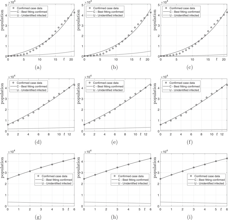
Let p be the number of data, Cdata and we take the most recent p data in Table 1. Fig. 3 shows the computational results with various N; and and 7. In this test, we consider three different N (i.e., ) to use the effective population appropriate to each situation. When investigating actual cases of epidemic spread, we can see that most infections have occurred in certain areas such as Wuhan in China rather than across the whole country, and then spread across the country. Therefore, it is good to choose an effective population size to suit the situation. As we can observe from the results of figures, if we use the recent small number of data, then we have better fitting results to the time series data. Furthermore, we can observe the number of the unidentified infected population decreases as time increases.
Fig. 3.
Computational results: (a), (b), and (c) are results with and ; (d), (e), and (f) are results with and ; (g), (h), and (i) are results with and .
Table 2 shows the computed numbers of unidentified infected population of COVID-19 on 11 February 2020 and a ratio β/γ. In a strict sense, the ratio is not equivalent to the basic reproduction number R 0 in the SIR model because our proposed model has a different meaning from the SIR model and we assume that the confirmed cases of infection are isolated completely from the susceptible population. Therefore, we present the ratio as a reference only.
Table 2.
Computed numbers of the unidentified infected patients of COVID-19 on 11 February 2020 and ratio β/γ.
| p/N | 109 | 108 | 107 |
|---|---|---|---|
| 22 | 5028 (1.10) | 5068 (1.10) | 1914 (1.04) |
| 14 | 3449 (1.04) | 3526 (1.04) | 1506 (1.02) |
| 7 | 2422 (0.93) | 2438 (0.93) | 2436 (0.94) |
Next, we perform the computational tests with various N and from 17 February 2020. Fig. 4 shows the computational results on 24 February 2020 with various N and . As shown in Fig. 4, we have the best fitting data of the confirmed cases. Table 3 shows the computed numbers of unidentified infected population of COVID-19 on 24 February 2020 and the ratio β/γ.
Fig. 4.
(a), (b), and (c) are results with and and 107, respectively, from 17 February 2020.
Table 3.
Computed numbers of the unidentified infected patients of COVID-19 on 24 February 2020 and ratio β/γ.
| p/N | 109 | 108 | 107 |
|---|---|---|---|
| 8 | 456 (0.61) | 423 (0.64) | 436 (0.63) |
4. Practical identifiability analysis
We perform the practical identifiability analysis of our proposed model using the Monte Carlo simulation (MCS) [19], [20]. We use the same data and parameter set as in Fig. 4. First, we solve the SUC model numerically with the obtained parameters β and γ; and obtain the vector Ci with for . Second, we generate Mparameter sets, (βj, γj) for . We take . Here, (βj, γj) are the optimized parameters with which the SUC model best fits with randomly perturbed confirmed data P i,jfrom Ci, where and for each j. σ 0 is the standard deviation. Third, we compute the average relative estimation errors (AREs):
| (10) |
Let us consider that a parameter is very sensitive to the noise. In [20], the parameter is not practically identifiable if ARE is higher than the measurement error σ 0. In this case, even with a moderate and reasonable level of measurement error, it may result in a seriously large ARE. Table 4 lists AREs for the parameters β and γ with respect to various noise levels σ 0. As expected, increasing σ 0 increases the AREs. Both the parameters β and γ are practically identifiable because the AREs are smaller than the measurement error σ 0. Therefore, the proposed model is practically identifiable, which implies the model parameters can be estimated from real data.
Table 4.
Average relative estimation errors for parameters β and γ.
| N | 109 |
108 |
107 |
|||
|---|---|---|---|---|---|---|
| σ0 (%) | ARE(β) (%) | ARE(γ) (%) | ARE(β) (%) | ARE(γ) (%) | ARE(β) (%) | ARE(γ) (%) |
| 0 | 0.00 | 0.00 | 0.00 | 0.00 | 0.00 | 0.00 |
| 1 | 1.87 | 1.26 | 0.87 | 0.57 | 0.48 | 0.37 |
| 5 | 3.98 | 2.93 | 2.54 | 1.82 | 1.54 | 1.36 |
| 10 | 6.02 | 4.64 | 4.15 | 3.25 | 2.82 | 2.59 |
| 20 | 10.03 | 7.87 | 7.93 | 5.95 | 5.42 | 4.67 |
| 30 | 13.65 | 11.23 | 10.55 | 9.80 | 7.29 | 7.91 |
5. Discussion
We proposed a new approach for modeling an epidemic disease, COVID-19, to estimate the unidentified infected case U. The proposed model is in a framework similar to the standard SIR model. However, our model suggests a different interpretation of a worldwide epidemic. The main purpose of the proposed model is to predict the number of the unidentified infected population who are infected but have not yet been confirmed.
The SUC model is potentially useful for determining the effectiveness of interventions. We can find out if various policy/strategy work well, and monitor their strengths and weakness by analyzing the changes of U after taking some actions. Furthermore, the model is helpful for predicting the extent of infection spread, i.e., U can be used as a criterion. Thus, we can prepare the proper quantity of protective masks or COVID-19 diagnostic kit to supply, hospital beds, medical staffs, and so on. It is significantly important to prevent the spread of infectious diseases and the incalculable damage caused by the epidemics.
However, the proposed model is as simple as possible under many constraints, assuming the ideal situation. In this paper, we reduced the complexity and focused on a basic building block. Thus, we excluded several realistic elements, for example, interventions, a latent period of virus, changes in population due to birth and death, infection in medical staff or confirmed patients not isolated, etc. In future works, we will complement various conditions for specific and realistic situations not covered in this paper to improve the model.
The accurate estimation of the unidentified infected using the proposed model depends on the reliable and accurate confirmed data. We used the number of the confirmed cases and deaths reported by WHO. There may be differences in how data is aggregated for each country or region. In fact, the criterion for classifying the confirmed cases in China has been changed twice, and it has led to sharp increase in the number of confirmed cases on 17 February 2020. Nevertheless, the proposed model can be modified by applying various situations for each system and culture in diverse countries. We only used the data on China, however, if the model is supplemented, it can be applied to many different countries with a variety of spread patterns.
6. Conclusion
The proposed SUC epidemic model for computing the unidentified infected for COVID-19 in China is very simple and is robust in computation. The model only uses the numbers of the total population and the available time series confirmed cases. The computational results from the model can be useful in controlling of the disease because we can estimate the size of the unidentified infected population. We performed the practical identifiability analysis of the proposed model using MCS. Finally, we clarified the importance of the proposed model and added its limitations. In the Appendix, we provide the source program code so that the interested readers can use and modify it for their own needs. In future works, we will improve the SUC model with more specific conditions such as a latent period, changes in population due to birth and death, infection in medical staff or confirmed patients not isolated. We will also develop a novel and proper index corresponding to the basic reproduction number used to investigate infectious diseases and compare to other diseases.
CRediT authorship contribution statement
Chaeyoung Lee: Methodology, Software, Validation, Formal analysis, Investigation, Data curation, Writing - original draft, Writing - review & editing, Visualization, Funding acquisition. Yibao Li: Validation, Investigation, Writing - original draft, Writing - review & editing, Funding acquisition. Junseok Kim: Conceptualization, Methodology, Software, Validation, Formal analysis, Writing - original draft, Writing - review & editing, Supervision, Funding acquisition.
Declaration of Competing Interest
The authors declare that they have no known competing financial interests or personal relationships that could have appeared to influence the work reported in this paper.
Acknowledgments
The first author (C. Lee) was supported by Basic Science Research Program through the National Research Foundation of Korea (NRF) funded by the Ministry of Education (2019R1A6A3A13094308). Y.B. Li was supported by the Fundamental Research Funds for the Central Universities (No. XTR042019005). The corresponding author (J.S. Kim) was supported by Korea University Future Research Grant. The authors are grateful to the editors and the reviewers for constructive and helpful comments on the revision of this article.
Appendix A
The following MATLAB codes are available from the corresponding author’s webpage:
http://elie.korea.ac.kr/cfdkim/codes/
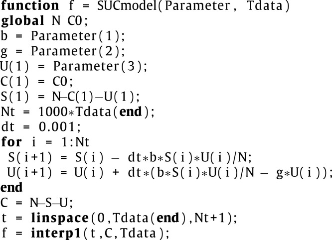
The following code is a function and should be saved with the file name ‘SUCmodel.m’ and placed in the same folder where the main code is.
 |
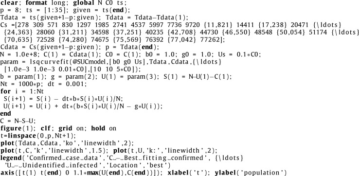
The following code is the main program.
 |
References
- 1.Zhao S., Musa S.S., Lin Q., Ran J., Yang G., Wang W., et al. Estimating the unreported number of novel coronavirus (2019-nCoV) cases in China in the first half of january 2020: a data-driven modelling analysis of the early outbreak. J Clin Med. 2020;9(2):388. doi: 10.3390/jcm9020388. [DOI] [PMC free article] [PubMed] [Google Scholar]
- 2.Novel Coronavirus (2019-nCoV) situation reports. Available online: https://www.who.int/emergencies/diseases/novel-coronavirus-2019/situation-reports/.
- 3.Anzai A., Kobayashi T., Linton N.M., Kinoshita R., Hayashi K., Suzuki A., et al. Assessing the impact of reduced travel on exportation dynamics of novel coronavirus infection (COVID-19) J Clin Med. 2020;9(2):601. doi: 10.3390/jcm9020601. [DOI] [PMC free article] [PubMed] [Google Scholar]
- 4.Roosa K., Lee Y., Luo R., Kirpich A., Rothenberg R., Hyman J.M., et al. Short-term forecasts of the COVID-19 epidemic in Guangdong and Zhejiang, China: February 13–23, 2020. J Clin Med. 2020;9(2):596. doi: 10.3390/jcm9020596. [DOI] [PMC free article] [PubMed] [Google Scholar]
- 5.Backer J.A., Klinkenberg D., Wallinga J. Incubation period of 2019 novel coronavirus (2019-nCoV) infections among travellers from Wuhan, China, 20–28 January 2020. Eurosurveillance. 2020;25(5):2000062. doi: 10.2807/1560-7917.ES.2020.25.5.2000062. [DOI] [PMC free article] [PubMed] [Google Scholar]
- 6.Hellewell J., Abbott S., Gimma A., Bosse N.I., Jarvis C.I., Russell T.W., et al. Feasibility of controlling COVID-19 outbreaks by isolation of cases and contacts. Lancet Glob Health. 2020;8(4):e488–e496. doi: 10.1016/S2214-109X(20)30074-7. [DOI] [PMC free article] [PubMed] [Google Scholar]
- 7.Tuncer N., Le T.T. Structural and practical identifiability analysis of outbreak models. Math Biosci. 2018;299:1–18. doi: 10.1016/j.mbs.2018.02.004. [DOI] [PubMed] [Google Scholar]
- 8.Chang H.J. Estimation of basic reproduction number of the middle east respiratory syndrome coronavirus (MERS-CoV) during the outbreak in South Korea, 2015. Biomed Eng Online. 2017;16(1):79. doi: 10.1186/s12938-017-0370-7. [DOI] [PMC free article] [PubMed] [Google Scholar]
- 9.Yang W., Cowling B.J., Lau E.H., Shaman J. Forecasting influenza epidemics in Hong Kong. PLoS Comput Biol. 2015;11(7):e1004383. doi: 10.1371/journal.pcbi.1004383. [DOI] [PMC free article] [PubMed] [Google Scholar]
- 10.Rao F., Mandal P.S., Kang Y. Complicated endemics of an SIRS model with a generalized incidence under preventive vaccination and treatment controls. Appl Math Model. 2019;67:38–61. [Google Scholar]
- 11.Reis R.F., de Melo Q.B., de Oliveira C.J., Gomes J.M., Rocha B.M., Lobosco M., et al. Characterization of the COVID-19 pandemic and the impact of uncertainties, mitigation strategies, and underreporting of cases in South Korea, Italy, and Brazil. Chaos Solitons Fractals. 2020;136:109888. doi: 10.1016/j.chaos.2020.109888. [DOI] [PMC free article] [PubMed] [Google Scholar]
- 12.Zhu L., Guan G., Li Y. Nonlinear dynamical analysis and control strategies of a network-based SIS epidemic model with time delay. Appl Math Model. 2019;70:512–531. [Google Scholar]
- 13.Kucharski A.J., Russell T.W., Diamond C., Liu Y., Edmunds J., Funk S., et al. Early dynamics of transmission and control of COVID-19: a mathematical modelling study. Lancet Infect Dis. 2020;20:553–558. doi: 10.1016/S1473-3099(20)30144-4. [DOI] [PMC free article] [PubMed] [Google Scholar]
- 14.Mizuno K., Kudo K. Proceedings of the international conference on social modeling and simulation, plus econophysics colloquium 2014. Springer, Cham; 2015. Spread of infectious diseases with a latent period; pp. 141–147. [Google Scholar]
- 15.Alam M., Tanaka M., Tanimoto J. A game theoretic approach to discuss the positive secondary effect of vaccination scheme in an infinite and well-mixed population. Chaos Solitons Fractals. 2019;125:201–213. [Google Scholar]
- 16.Rosa S., Torres D.F. Optimal control of a fractional order epidemic model with application to human respiratory syncytial virus infection. Chaos Solitons Fractals. 2018;117:142–149. [Google Scholar]
- 17.Rihan F.A., Al-Mdallal Q.M., AlSakaji H.J., Hashish A. A fractional-order epidemic model with time-delay and nonlinear incidence rate. Chaos Solitons Fractals. 2019;126:97–105. [Google Scholar]
- 18.López C.P. MATLAB optimization techniques. Apress; Berkeley, CA: 2014. Optimization techniques via the optimization toolbox; pp. pp.85–108. [Google Scholar]
- 19.Miao H., Xia X., Perelson A.S., Wu H. On identifiability of nonlinear ODE models and applications in viral dynamics. SIAM Rev. 2011;53(1):3–39. doi: 10.1137/090757009. [DOI] [PMC free article] [PubMed] [Google Scholar]
- 20.Tuncer N., Marctheva M., LaBarre B., Payoute S. Structural and practical identifiability analysis of zika epidemiological models. Bull Math Biol. 2018;80(8):2209–2241. doi: 10.1007/s11538-018-0453-z. [DOI] [PubMed] [Google Scholar]


