PunctaSpecks: A Tool for Automated Detection, Tracking, and Analysis of Multiple Types of Fluorescently Labeled Biomolecules

Abstract

Recent advances in imaging technology and fluorescent probes have made it possible to gain information about the dynamics of subcellular processes at unprecedented spatiotemporal scales. Unfortunately, a lack of automated tools to efficiently process the resulting imaging data encoding the fine details of the biological processes remains a major bottleneck in utilizing the full potential of these powerful experimental techniques. Here we present a computational tool, called PunctaSpecks, that can characterize fluorescence signals arising from a wide range of biological molecules under normal and pathological conditions. Among other things, the program can calculate the number, areas, life-times, and amplitudes of fluorescence signals arising from multiple sources, track diffusing fluorescence sources like moving mitochondria, and determine the overlap probability of two processes or organelles imaged using indicator dyes of different colors. We have tested PunctaSpecks on synthetic time-lapse movies containing mobile fluorescence objects of various sizes, mimicking the activity of biomolecules. The robustness of the software is tested by varying the level of noise along with random but known pattern of appearing, disappearing, and movement of these objects. Next, we use PunctaSpecks to characterize protein-protein interaction involved in store-operated Ca²⁺ entry through the formation and activation of plasma membrane-bound ORAI1 channel and endoplasmic reticulum membrane-bound stromal interaction molecule (STIM), the evolution of inositol 1,4,5-trisphosphate (IP₃)-induced Ca²⁺ signals from sub-micrometer size local events into global waves in human cortical neurons, and the activity of Alzheimer’s disease-associated β amyloid pores in the plasma membrane. The tool can also be used to study other dynamical processes imaged through fluorescence molecules. The open source algorithm allows for extending the program to analyze more than two types of biomolecules visualized using markers of different colors.

Graphical Abstract

Introduction

Recent advances in imaging techniques for visualizing biological processes at unprecedented spatiotemporal scales ranging from single molecule to whole-cell signals have revolutionized biological research [1–5]. It is now possible to study dynamical processes such as the flux through individual ion channels, diffusion of proteins in cell membrane, and movement of motor proteins and filaments along microtubules [6–11]. These experiments often generate huge amount of imaging data on the dynamics of hundreds or thousands of such objects (terms objects, puncta, or events are used interchangeably throughout the manuscript) that needs to be analyzed quantitatively and efficiently to reveal their functional properties. Manual or semi-automatic analysis of these data sets is labor intensive, costly, inaccurate, and poorly reproducible, undermining the usefulness of technological advances. Thus, automated analysis of the data to extract quantitative information about the dynamics of the underlying biological processes is imperative.

Depending on the biological question being asked, fluorescence imaging data from a wide range of experimental scenarios such as single and multiple types of objects, variable particle density, and congested physiological environments (noise) need to be processed. These objects can be proteins tagged with fluorescent proteins or labeled by staining with specific dyes. More often these processes evolve in time and space. For example, Ca²⁺ release events evolve from blips or quarks due to opening of individual channels for a few milliseconds to micrometer-sized puffs and sparks caused by the concerted opening of a few closely located channels for hundreds of milliseconds to whole-cell waves lasting for minutes [12]. Imaging experiments record these events and their progression in a noisy cellular environment by recording changes in cell fluorescence overtime [13–17]. A high throughput analysis of these events is key for understanding their function and specificity [12, 18, 19].

Some biological processes, on the other hand, remain confined to a very small space. They are short lived and can coexist in a large number. Yet, their dynamics have crucial implications for the cell function and survival. For example, cation-permeable pores formed by soluble beta amyloid (Aβ) aggregates in the cell membrane can destabilize the cell ionic homeostasis, and are believed to contribute to the pathology of Alzheimer disease [20–24]. The activity and evolution of these pores is often recorded in multi-gigabyte image stacks using high throughput, massively parallel optical patch clamp technique [8, 25]. Analyzing the spatiotemporal dynamics of localized events as they evolve into global signals or thousands of small spatially confined, short-lived events require accurate and efficient numerical methods.

In some situations, fully understanding a biological process requires characterizing the collective or concurrent behavior of more than one type of molecules or reactions visualized using markers of different colors. For instance, store operated Ca²⁺ entry (SOCE) refers to a process by which Ca²⁺ channels localized in the plasma membrane (PM) are activated when luminal Ca²⁺ stores in the endoplasmic reticulum (ER) are depleted. In many cells, SOCE is mediated by the highly Ca²⁺-selective plasma membrane channel, ORAI1, and the ER-resident Stromal Interaction Molecules (STIM1 and STIM2) that sense changes in the Ca²⁺ concentration of the ER lumen ([Ca²⁺]_ER). ORAI1 and STIM1/2 are labelled with two different fluorescent tags to record their activity simultaneously. Following cell stimulation that results in [Ca²⁺]_ER reduction, STIMs aggregate and translocate to the ER-PM junctions where they recruit and activate ORAI1. These junctions are sites where the ER membrane is closely apposed to the PM. Localization of ORAI1 with STIMs in these junctions compartmentalize the Ca²⁺ signaling machinery to discrete sites where the Ca²⁺ signals generated are channeled to activate distinct downstream cellular processes. This ensures the high signaling fidelity of responses triggered by ORAI1-mediated Ca²⁺ signals from the ER-PM junctions [26–29]. The movement of these proteins in live cells following cell stimulation has been reported using various imaging techniques, such as confocal and total internal reflection fluorescence (TIRF) microscopy. The time-lapse image stacks acquired over several minutes show that they are highly dynamic and mobile following stimulation.

As mentioned above, the high-resolution imaging experiments record the activity of many objects or events usually immersed in a physiologically dense environment, introducing background noise during image acquisition. While the background noise can be removed, delineating individual objects or events and tracking their movement, amplitudes, spatial sizes, and lifetimes over time remains a major challenge. These types of data-sets demand efficient automated tools for accurately identifying and tracking the dynamics of each object over time to elucidate the underlying biological processes. A number of tools have been developed over the past either de novo or adapting preexisting tools tailored for the specific problem [24, 30–39]. In particular, several tools for analyzing localized Ca²⁺ signals in cardiac myocytes have been developed over the years [40–47].

Due to the diverse spatiotemporally dynamical nature of the biological processes, there does not exist a “one-size-fits-all”, universally applicable method. Therefore, specialized tools tailored to address the problem at hand is often the way to go. We have developed an all-in-one MATLAB-based tool called PunctaSpecks, with a graphical user interface (GUI), that implements algorithms for identifying and characterizing fluorescently labeled objects in time-lapse image stacks. PunctaSpecks generates outputs that report on the distributions of spatial sizes, amplitudes in terms of mean or maximum intensity, mean active times, mean silent times, mobility patterns, and time-resolved trajectories of all objects or events in the recording, and overlap probabilities of two different types of objects such as ORAI1 and STIM in a given frame. We have implemented a variety of algorithms for preprocessing these movies to identify objects and extract their features of interest. A range of options are available to perform various analysis tasks on the identified objects and export data for later analysis. The open source MATLAB algorithm can be modified to analyze more than two types of biomolecules visualized using markers of different colors.

Methods

To process time-lapse images containing the dynamics of up to two biomolecules or processes, we have developed PunctaSpecks using MATLAB Version 9.5 and Image Processing Toolbox Version 10.3. PunctaSpecks is a GUI-driven application. A User Manual with step by step instructions and the software are given in the Supplementary Information. Below we describe the main features of the program.

Algorithms and Features Incorporated in PunctaSpecks

Graphical User Interface (GUI)

The MATLAB GUI for PunctaSpecks has multiple tabs, where similar tasks are grouped under the same tab, with various processing steps divided into different categories on each tab. The first tab in the GUI is the GENERAL tab with different options such as LoadFiles, Pre-Processing, Threshold Selection, Calculate ROIs, Puncta Trajectories lists, ShowAllPunctas, and Image Panels to show pre- and post-processed movie stacks (Figure S1 in User Manual). After the program starts, pressing the LoadFiles button enables the user to load time-lapse image stacks (in TIFF format) for up to two different types of recorded objects, which are displayed in the top two image panels. After loading the image stacks, a pop-up panel shows the Maximum Intensity Profile (MIP) image for each stack to provide a global perspective of all potential regions of interest in the entire movie.

As PunctaSpecks can process data from various experimental sources, a “Pre-processing” step may be required to remove background noise or artifacts before applying any object detection algorithm. PunctaSpecks provides two image smoothing algorithms, a combination of Median and Gaussian filters and Otsu method (Figure S1 in User Manual). These can be applied individually or together based on the quality of the images. After selecting the Smoothing Filters radio button, a dialogue box appears to allow the user to choose an algorithm and adjust its parameters to get a filtered image stack (Figure S3A in User Manual). The filtered images are used in subsequent processing steps.

Following the pre-processing step are a range of options for threshold selection. The user can select various thresholding options including Region, Frame, Otsu, Laplacian of Gaussian (LoG), and Difference of Gaussians (DoG) methods. The “Region” option allows the user to draw a region of interest (ROI) on the image background, where the pixel values within the ROI will be subtracted from all pixels in the image stack. The “Frame” option allows the user to select an image frame that will be subtracted from all other frames in the image stack. The Otsu Method uses the Otsu algorithm to threshold the image to isolate the signal from the background. Otsu thresholding can be done using the stack histogram or frame wise [48]. Other options that use more advanced thresholding algorithms such as LoG and DoG are also included [49–51]. In order to evaluate the effectiveness of the algorithm, each panel shows original and processed images. For example, in the case of Otsu method a dialogue box is provided to further select the frame-wise or multi-stack Otsu method with values shown in the top panel of Figure S3B in User Manual. Similarly, in case of LoG and DoG dialogue boxes (Figure S4 in User Manual), options to change algorithm parameters are also provided. After selecting the appropriate options and pressing “Apply” button, the resulting filtered images are displayed in the same dialogue box along with the original images. A panel with a MIP image showing puncta or objects identified appears to assess the effectiveness of the algorithm (Figure S3C in User Manual). In case of LoG and DoG, the second panel show the filtered images, while the bottom panel display the objects identified for assessment (Figure S4 in User Manual). If user is not satisfied with the results, the parameters or threshold values can be adjusted. The slider bars under the images allow for evaluating the identified puncta after thresholding. After closing this dialogue box, processed image stacks are shown in the main GUI. Pressing “Calculate ROIs” button then runs another algorithm where information about each object in each frame in the image stack(s) are stored for later processing.

The RESULTS tab (Figure S5 in User Manual) provides different buttons to retrieve various statistics about the identified puncta. These include calculating the Pearson’s Correlation and Mander’s Overlap Coefficients for puncta in two consecutive frames of a single movie or frames of two movies recorded simultaneously having information about two different types of objects or puncta (PCC_Mander), analysis for all puncta detected in each frame (ROI Stats), overlap probabilities between puncta in two movies recorded simultaneously (OverlapP), dwell times in active and inactive states of all puncta (DwellTime), and trajectories of mobile objects (PunctaMobility). Different Excel spreadsheets (in comma separated value (CSV) format) containing results from various calculations are also generated (see User Manual for more details) for later use. When each button is pushed, a summary of the properties calculated is shown as line graphs over time and/or histograms/bar graphs.

Finally, the SUMMARY tab contains the overall statistics of various properties calculated in the RESULTS section (Figure S7 in User Manual). These include the histograms for the number of objects per frame (ROIs/frame), average intensity of all puncta per frame (AvgI/puncta), and total area of all puncta in a frame for each image stack. This information is also tabulated for each movie stack in the SUMMARY. Information about the types of puncta (mobile, stationary etc.) in the entire image stack are also tabulated. Average statistics of puncta on frame-by-frame basis are also tabulated. Please note that PunctaStatics button on the SUMMARY tab is enabled only if user has performed ROI stats and PunctaMobility operations on the RESULTS tab.

If the PunctaMobility function under RESULTS is used, trace of each mobile punctum in either of the movies can be seen on the GENERAL tab (Figure S6 in User Manual). Once a punctum is selected from the drop-down list, it is shown as red circled puncta in the respective movie panel in the bottom row. Generally, all Immobile puncta are encircled by green circles and mobile puncta are encircled by red circles. “ShowAllPuncta” button can be used to highlight the mobile (in red) and immobile (in green) puncta for each frame of the image stack after the list of all particle trajectories has been generated in the RESULTS tab.

Punctum Object Detection

Typically, fluorescently labeled objects immersed in a noisy background are identified using various standard image processing steps [52–54]. The noise and drifting background in the imaging data result from the movement or dynamics of biological objects in congested cellular environment and time-dependent system biases. Proper identification and tracking of these fluorescently labeled objects or events in time-lapse experiments is always challenging. PunctaSpecks uses a series of steps to overcome these challenges.

Figure 1A shows a typical image stack (in this case a synthetic movie stack containing circle-like objects) often consisting of several hundred frames (only five frames with two moving puncta are shown here). Each frame is taken at a fixed time interval (called frame rate) showing the dynamic activity of the processes under study. Since a biological system is mostly dynamic with different events happening over time, we get a general sense of the activities of all objects by obtaining a MIP image of the stack. We record the highest intensity of a given pixel over the entire movie, repeating this procedure for all pixels. The resulting image is called MIP where each pixel represents the highest intensity observed at the pixel over time (Figure 1B). Notice that there are only two puncta in the first five frames of the movie shown in Figure 1A but MIP image shows all the puncta in the entire movie.

Figure 1.

Various steps used by PunctaSpecks for noise removal and puncta identification. (A) Synthetic movie stack containing dynamical activity of objects under investigation (only 5 frames are shown). (B) Maximum intensity profile (MIP) image of the whole movie. (C) Puncta identified by PunctaSpecks using a given algorithm (Otsu in this case) are encircled on the MIP image to ease the visualization and further adjustment of parameters for accurate detection of all puncta. Histograms of the areas (D), mean fluorescence intensity (E) of all puncta, and (F) mean square displacement as a function of time for the mobile puncta.

The next step is to isolate the puncta from the background by selecting appropriate smoothing and thresholding method to remove noise and artifacts. In the pre-processing step, the user is provided with the option of combining Median and Gaussian filtering with global Otsu thresholding for image smoothing and blurring. Note that not all movies require this step but the user is encouraged to evaluate whether pre-processing an image stack improves the quality of object detection in the subsequent thresholding step. Several algorithms for threshold identification are provided to handle the widely encountered scenarios. These include removal of the first frame (assumed to be representative of noise throughout movie) from the entire movie (radio button Frame) or using the maximum, mean, or minimum intensity values of pixels in a ROI drawn by the user to correct for the background noise in each frame (radio button Region). Other options that use more advanced thresholding algorithms include the Otsu method, as well as LoG and DoG filters. The Otsu method utilizes a binarization algorithm to conduct frame-wise or global (using the stack histogram) noise removal [48]. LoG and DoG are sophisticated filters used to reduce a noisy background and detect the edges of geometrically round objects [49–51].

After applying the appropriate thresholding method, all identified puncta are encircled on the MIP image or shown on the processed images in the dialogue box used for applying the thresholding filter to ease the visualization (for example, see Figure 1C). Puncta identified in each frame can be viewed using the scroll bar below the processed images under GENERAL tab (Figure S1–4 in User Manual). These ROIs are used in the next step to quantify various parameters such as the distribution of sizes (Figure 1D) and mean intensities (Figure 1E) of all puncta, and their diffusivity (Figure 1F).

Puncta Characterization

After identifying the puncta, we next retrieve various statistics using MATLAB functions bwlabel and regionprops that provide insights into biological questions at hand such as channel kinetics and protein-protein interactions before and after stimulation. Pressing “Calculate ROIs” (Figure S1 in User Manual) button calculates various parameters such as area, maximum and mean intensity, pixel coordinates and center of mass coordinates for each punctum. When two fluorescent proteins are expressed in the same cell, calculating Pearson Correlation Coefficient (PCC) between two frames in the two movies (the first movie frame representing one protein and the second movie frame representing the other protein) recorded simultaneously allows us to visualize how protein-protein correlation changes over time (“PCC_Mander” button in “Results” tab, Figure S5 in User Manual). PunctaSpecks also calculates PCC between two consecutive frames for each individual protein or object. In general, positive PCC indicates a positive correlation, whereas a negative or close to zero value indicate an inverse or no correlation. For each individual protein, PCC between two frames suggests how protein dynamics changes over time in the cellular area of interest. This way, movement of the protein either into or out of this area, activation of the protein in a new region, or deactivation of the protein in an existing region can be quantified. When two proteins are co-expressed, PCC between the two image stacks shows how protein-protein interaction changes with time. In addition to Pearson, “PCC_Mander” button also calculates the Mander’s Overlap Coefficient (MOC) between two different proteins to quantify protein co-localization or co-occurrence within the same ROI [55].

The “ROI Stats” button generates CSV files for each frame in the image stack and outputs the values for maximum and mean fluorescence intensity, size or area (in pixels), and the (X, Y) coordinates for each punctum detected. While calculating the MOC is a better method to identify the extent of overlap between two fluorescently labeled protein, PunctaSpecks also provides another method to calculate the physical overlap or spatial correlation between puncta using the “OverlapP’ button. Additionally, the “DwellTime” button calculates the duration for which the punctum or ROI appears (Figure S5 in User Manual). Upon completing the respective calculations by pushing each button, outputs are saved as CSV files that can be easily used in other software such as Excel, Python, R, and Fiji [36] for further analysis. By default, each file name is prefixed with the names of the movie files (see User Manual). Some general data files are stored even though if user cancels the file storing options. In addition to generating CSV files, PunctaSpecks also summarizes the results from each calculation as histograms and/or line graphs (see for example, Figure 1D).

Puncta Tracking and Diffusion

Single particle tracking, especially in the context of living cellular systems is challenging due to the dense intracellular environment and dynamics of the tracked particles. This is further complicated by the ability of objects to aggregate, split, and merge. As mentioned above, after thresholding the movie, PunctaSpecks uses MATLAB functions bwlabel to get 8-connected components for each frame and regionprops to gather region-specific information like area, maximum and mean intensity, coordinates of all pixels in an ROI and its center of mass. All tracking and diffusion calculations are based on this data. Therefore, it is important to properly delineate the individual puncta using the appropriate thresholding method as poor thresholding may result in large number of falsely identified objects, leading to inaccurate measurements that can slow down all subsequent calculations. Setting the threshold too high compromises the quality of results as many biologically relevant particles may be inadvertently discarded.

“PunctaMobility” button is used to track each punctum and classify it into one of the three categories: (1) immobilel - a punctum that appears in more than one frames at the same location with no change in its size; (2) immobile2 – a punctum that appears in only one frame, including that with increasing/decreasing size while staying at the same position; and (3) mobile – a punctum that overlaps with another punctum in the next frame by a user-specified threshold (default = 0.1). Note that mobility of the punctum can change with time in a given experimental condition. A mobile punctum may also have stationary states known as gaps, which can last for an indefinite duration and may represent a situation where the mobile punctum has been immobilized. The reasons for this can vary as it depends on the nature of the proteins being examined and cellular context in which the experiments are being done.

Next, a single particle trajectory for each mobile punctum is calculated by following its center of mass. From these trajectories, various mobility parameters such as net displacement of a punctum, mean square displacement, diffusion coefficient [56, 57], and mean diffusion coefficient of an ensemble of trajectories (Figure 1F) are calculated. Trajectory representing the location of the center of mass of each identified mobile punctum can be viewed by selecting that punctum in the GENERAL tab (Figure S6 in User Manual). Note that once a punctum from one of the two dropdown lists is selected to view its trajectory, the dropdown list for the other movie file is disabled. “ShowAllPunctas” button can be used to enable both lists again. The trajectories graph for a few puncta are also shown in the RESULTS tab as examples. All trajectories are saved as a CSV file for further processing and plotting. We also save each trajectory as individual CSV file that can be easily loaded into Fiji/ImageJ [58] to visualize the movement of a particle being tracked.

Data Records

We apply our program to synthetic data and experimental data sets from TIRF microscopy experiments. Our experimental data sets comprise three examples, representing the activity of ORAI1/STIM1 in HEK293 cells, IP₃-mediated local and global Ca²⁺ signals in human cortical neurons, and the gating of Aβ-induced Ca²⁺-permeable pores in Xenopus oocytes [21].

Synthetic Data

Synthetic data was generated using MATLAB in the form of a movie file comprising of several hundred frames each having size 182 × 254 pixels. Puncta of random sizes ranging from 5 to 100 pixels were placed at random locations. Uniformly distributed noise of various strengths ranging from 25 to 150 (in increments of 25) intensity units (where the maximum signal intensity is 255 units) was introduced to each frame. This way, we have generated 6 synthetic data sets with first set having noise strength of 25 and last synthetic data set have noise strength of 150. This gives data sets with signal to noise ratio (SNR) in the range of 7.5 to 1 (Figure 2A). Assuming a noise n(i,j) and a real signal s(i,j) at location (i,j), the final image is given by:

$$f(i,j)=s(i,j)+n(i,j).$$

SNR of a given image is defined as,

$$\mathit{SNR}=\sqrt{\frac{{\sigma }_f^2}{{\sigma }_n^2}-1}.$$

Where ${\sigma }_f^2$, ${\sigma }_s^2$ and ${\sigma }_n^2$ are the variances of final image, signal, and noise respectively

$${\sigma }_f^2={\sigma }_s^2+{\sigma }_n^2.$$

Figure 2.

Verifying the performance of PunctaSpecks using synthetic data. (A) Frame-by-frame signal to noise ratio of the synthetic data at two different noise levels. Histograms of areas (B), mean open times (log scale) (C), and dwell times (log scale) (D) of all puncta with true (blue) and those from PunctaSpecks at noise levels 25 (green) and 150 (red). (E) Histogram of mean intensities of all puncta with true values (blue) and those from PunctaSpecks at noise level of 25 (green) and 150 (red). The actual trajectory of a sample mobile punctum (blue) and the one identified by PunctaSpecks at noise level of 150 (red) (F).

To mimic random appearances and disappearances of puncta, we used 5 events per punctum with open and close times drawn randomly from a uniform distribution in the range of 2 to 20 ms (considering 1 frame/ms recording frequency) for open times and up to 80 ms for close times. To test for tracking the diffusion and movement, a known but random displacement of predefined length is applied to different puncta during their open time intervals.

Experimental Methods for ORAI1 and STIM1 Activity

Cell Culture and Transfection:

HEK293 cells were maintained in DMEM supplemented with 10% heat-inactivated fetal bovine serum, 1% glutamine, and 1% penicillin/streptomycin (37°C; 5% CO₂) (All solutions from Life Technologies, Grand Island, NY). Cells were transfected with the required constructs as described in the text using Lipofectamine 2000 (Life Technologies). The transfected cells were maintained in Opti-MEM medium (Life Technologies) for 3 h, at the end of which the transfection mix was replaced with complete DMEM. Cells were used 24 h after transfection. All other reagents used were of molecular biology grade obtained from Sigma-Aldrich (St. Louis, MO) unless mentioned otherwise.

DNA Constructs:

YFP- and CFP-tagged STIM1/STIM2 constructs were obtained from Tobias Meyer (Stanford University, Stanford, CA). YFP-tagged Orail was obtained from Tamas Balia (NICHD, NIH).

TIRF Microscopy:

HEK293 cells were plated on collagen-coated glass-bottomed tissue culture dishes (MatTek Corporation, Ashland, MA), transfected as required and used 24 h later. TIRF imaging was performed using an Olympus IX81 motorized inverted microscope (Olympus, Center Valley, PA) with a TIRF-optimized Olympus Plan APO 60× (1.45 NA) oil immersion objective and Lambda 10-3 filter wheel (Sutter Instruments, Novato, CA, USA) containing 480-band pass (BP 40 m) and 540-band pass (BP 30 m) emission filters (Chroma Technology, Bellows Falls, VT). Images were collected using a Hamamatsu ORCA-Flash4.0 camera (Olympus) and the MetaMorph imaging software (Molecular Devices, Downingtown, PA).

Experimental Methods for IP₃-Induced Ca²⁺ Signals in Human Cortical Neurons

Cell Cultures:

Neuronal cultures were established from 16-21-week-old human fetal brain tissue specimens as previously described [59]. Tissue procurement and use complies with all federal and institutional guidelines; informed consent signed by all interested parties. The cells were plated on PEI-covered glass coverslips and maintained in vitro in DMEM supplemented with 10% FCS.

Ca²⁺ Imaging and Data Analysis:

Neurons were loaded with combination of Fluo-4 AM (20 μM) and membrane-permeant caged IP₃-AM (4 μM for 1 h at RT in Ca²⁺-HBSS). Cells were bathed in extracellular saline solution (PBS) containing 2 mM Ca²⁺ during the imaging. IP₃ was photoreleased upon UV light flash of different durations. Changes in the intracellular Ca²⁺ concentration were measured using 488 nm argon–ion laser for fluorescence excitation, and a CCD camera for imaging fluorescence emission (510 – 600 nm) at frame rates of 30 to 100 s⁻¹. MetaMorph was used for acquisition and analysis of global and local Ca²⁺ responses. Fluorescence is expressed as ratio of mean change in fluorescence (ΔF) at each pixel relative to the resting fluorescence (F₀).

Experimental Methods for Ca²⁺-Permeable Plasma Membrane Aβ Pores Activity

Oocyte Preparation and Electrophysiology:

Solution containing soluble oligomers prepared from human recombinant Aβ42 peptide and aliquots were applied using a glass pipette with tip diameter of ~30 μm to voltage-clamped oocytes of defolliculated stage VI Xenopns laevis injected with fluo-4 dextran [21]. For imaging, oocytes were placed animal hemisphere down in a chamber whose bottom is formed by a fresh ethanol washed microscope cover glass (type-545-M; Thermo Fisher Scientific) and were bathed in Ringer’s solution (110 mM NaCl, 1.8 mM CaCl₂, 2 mM KC1, and 5 mM Hepes, pH 7.2) at room temperature (~23°C) continually exchanged at a rate of ~ 0.5 ml/min by a gravity-fed superfusion system. The membrane potential was clamped at a holding potential of 0 mV using a two-electrode voltage clamp (Gene Clamp 500; Molecular Devices) and was stepped to more negative potentials −100 mV when imaging Ca²⁺ flux through Αβ pores to increase the driving force for Ca²⁺ entry into the cytosol.

TIRF Microscopy Imaging:

Fluorescence produced by laser-agitated fluor-4-dextran binding to the Ca²⁺ flowing through the open Aβ pores was observed using an Olympus IX 70 microscope and Olympus 60x TIRFM objective (NA = 1.45) and a cooled, back-illuminated CCD (Cascade 128+, Roper Scientific). Excitation was provided by 488nm argon ion laser, brought to bear on the extreme edge of the specimen. With this setup, the CCD produces full frame 128x128 pixel images (0.33 μm per pixel) captured every 2 ms. Metamorph (Universal Imaging) was used to capture these frames in real time so that they may be stored on disk for later processing.

Results

We first test the robustness of PunctaSpecks using synthetic data sets generated with varying SNR from <1 to 7.5. Here we report our analysis for the movies with the lowest and highest SNR. In both cases, the movie has 327 frames with 493 puncta. Out of these 493 puncta, 11 were mobile. In Figure 2A, we show the frame-by-frame SNR with noise level of 25 and 150. PunctaSpecks accurately identified all puncta and their areas in both cases (Figure 2B), as well as calculated the mean active times (τ_o) and dwell times of these puncta (Figure 2C, D). The mean intensity identified by PunctaSpecks also matches very well with the true values (Figure 2E). The slight discrepancy in the intensity values come from the fact that fluorescence is derived from uniformly distributed pixel values while generating the data. We remark that the discrepancy between the actual puncta properties and those estimated by PunctaSpecks increases as we decrease the SNR further. However, we omit those results because the SNR of most fluorescence microscopes is much higher than 1 (for example, see [60]). PunctaSpecks was also able to identify the trajectories of all puncta at both noise levels generated (the actual and detected trajectory of a sample object at the noise level of 150 is shown in Figure 2F).

Assessing the Dynamics of STIM1 and ORAI1 During SOCE

To assess how PunctaSpecks handles real biological data, we processed different time-lapse image stacks that show the activation and movement of ORAI1 and STIM1 proteins after stimulation with cyclopiazonic acid (CPA) to inhibit Ca²⁺-ATPase in the ER and allow passive depletion of the ER-Ca²⁺ stores. As described above, these images were acquired using TIRF microscopy [61], where the incoming excitation laser does not directly illuminate the sample but is bent to illuminate the sample at a certain angle to produce an evanescent wave that excites the fluorophores. In TIRF, only fluorophores found at close proximity (usually up to 100nm) to the glass coverslip are excited. This technique produces images with very low background and greatly improved SNR with almost no interference from out-of-focus fluorescence [62]. The TIRF images shown here were obtained from HEK293 cells expressing fluorescently-tagged ORAI1 and STIM1 proteins.

Figure 3 shows the formation of STIM1 and ORAI1 puncta as a function of time. As can be seen in the grayscale images, there was no obvious puncta for both Orail and STIM1 in the beginning before stimulation (only ORAI1 is shown in Figure 3A). Following stimulation with CPA, STIM1 and ORAI1 start aggregating in the ER-PM junctions and these aggregates are visualized as puncta (Figure 3B and C). PunctaSpecks was able to capture these changes as shown by the line graphs in Figure 3D–F. The number of puncta for both STIM1 and ORAI1 increases (Figure 3D) after CPA stimulation over the duration of the experiment, as did their mean fluorescence intensities (Figure 3E), and mean area (the number of pixels per punctum) (Figure 3F). We would like to point out that before stimulation, STIM1 is tracking along the microtubules via its association with EB1 at the plus ends. Following stimulation, STIM1 starts aggregating to form puncta. As we highlighted further in the “Discussion” section, PunctaSpecks is not able to differentiate between STIM1 moving along the microtubules and that in the punctum form. The changes in average area for STIM1 in the beginning reflects the initial detection of moving STIM1, which can be in large numbers and are found all over the cell. The dip in average area after stimulation could represent the decreased movement of STIM1 as puncta start to form. As more puncta emerge over time, the average puncta area increases.

Figure 3.

Formation of STIM1 and ORAI1 puncta after stimulating HEK293 cells with cyclopiazonic acid. (A-C) Snapshots of the ORAI1 activity at the beginning (before stimulation), middle and end of the experiment (after stimulation). The number of puncta formed (D), mean intensity per punctum (E) and average area per punctum (F) as a function of time for STIM1 (blue) and ORAI1 (red).

The mobility of STIM1 and ORAI1 from the experiments described in Figure 3 is shown in Figure 4. An example trajectory for STIM1 (Figure 4A) and ORAI1 (Figure 4D) along with mean square displacement versus time averaged over more than 50 such trajectories (Figure 4B, E) are also shown. Mean of the diffusion coefficient (of all these trajectories) for STIM1 is 0.0022 μm²/sec and for ORAI1 is 0.0029 μm²/sec (Figure 4B, E). Note that the mean values are for the entire time series. Figure 4C shows that significant physical overlap between STIM1 and ORAI1 puncta starts as early as 150 s, indicating early interaction events between the two proteins. Furthermore, co-occurrence analysis [55, 63] with respect to fluorophores intensity (also called MOC) of the two types of puncta reveals that ORAI1 puncta are completely immersed in STIM1 puncta (Figure 4F).

Figure 4.

Mobility of STIM1 and ORAI1 after stimulating HEK293 cells with cyclopiazonic acid. An example trajectory (A) and mean square displacement versus time for all mobile STIM1 puncta (B). (D, E) Same as (A, B) for ORAI1. (C) Time-series of the overlap probability of STIM1 and ORAI1 puncta. (F) Mander’s overlap coefficients for STIM1 in ORAI1 (blue) and vice versa (red).

To visualize how different options for Threshold Selection will affect the results, the same ORAI1 and STIM1 image stacks analyzed earlier using the Otsu method were re-analyzed with the LoG or DoG filters (Figure 5). For both proteins, minimal changes were observed in the number of puncta detected and mean puncta intensity. Nonetheless, delineation of puncta edges differed between these options, as shown by the calculated average puncta area over time. The LoG filter appeared to yield the smallest amount of variability for average puncta area (indicated by the bars showing standard error of the mean (SEM)).

Figure 5.

Comparison of the Otsu, LoG, and DoG methods for Threshold Selection. (A-C) snapshots of the image frames at the beginning, middle and end of the experiment of ORAI1. Time traces of the activity of ORAI in terms of the number of puncta formed (D), mean intensity of puncta (E) and average area per punctum (F). Lower panel (G-I) reports similar data for STIM1.

Next, we test the robustness of PunctaSpecks further by analyzing two images stacks of STIM1 where the cell is either stimulated with CPA (25 μM) or non-stimulated. As shown in Figure 6 (red traces), CPA-treated cells exhibited significantly higher puncta number, mean intensity, and average area of puncta when compared to non-stimulated cells. The fluctuations in mean puncta intensity values for STIM1 in the beginning of the experiment are due to the detection of STIM1 moving along the microtubules before cell stimulation. CPA induced a substantial depletion of the ER-Ca²⁺ stores that triggered the aggregation of STIM1 in ER-PM junctions to form puncta. As more STIM1 aggregated within these junctions, there was less of the protein moving along the microtubules. Hence, the mean fluorescence intensity for STIM1 puncta was more stable during the latter part of the time series, compared to the time period before stimulation (Figure 6). Similarly, average STIM1 puncta size was more stable towards the end of the time series when compared to the beginning (Figure 6C, red trace). In contrast, without any stimulation, no appreciable increase was observed in the number or average area of the puncta, as well as mean fluorescence intensity. The fluctuations in mean fluorescence intensity is primarily due to STIM1 tracking along the microtubules (Figure 6, black traces).

Figure 6.

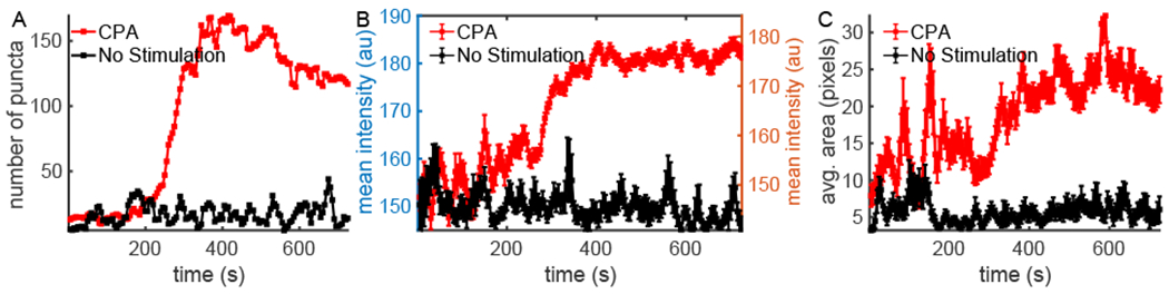
Comparison of STIM1 without stimulation and when stimulated with CPA (25 μM). The number (A), mean fluorescence intensity (B), and average area (C) of puncta as a function time in HEK293 cells without any stimulation (black) or treated with CPA (red).

Evolution of IP₃-Induced Ca²⁺ Signals in Human Cortical Neurons

One of the key features of PunctaSpecks is that it can track how different properties of objects or events evolve over time. This is crucial for gaining insights into biological processes where local events recruit nearby sites to form a global event or a global event disintegrates into many small events. A typical example of this behavior is the hierarchical Ca²⁺ signals in the cell where Ca²⁺ release due to a single channel (quarks or blips) recruit nearby channels to give rise to a slightly bigger event called a spark or puff. In certain situations, sparks or puffs coordinate throughout the cell to result in a global Ca²⁺ wave. Our tool enables us to quantify the properties of local events that eventually lead to global events and vice versa. As an example, we apply PunctaSpecks to study the activity of IP₃-induced Ca²⁺ signals in human cortical neurons. Figure 7 shows the activity of a single IP₃R and a puff due to concerted opening of multiple channels in a cluster (Figure 7A) in the beginning of the experiment that recruit more neighboring puff sites later (Figure 7B). Several discrete Ca²⁺ puffs eventually lead to a global wave spreading over the entire neuron towards the end of the experiment (Figure 7C). Note that PunctaSpecks identify all discrete events leading to a global wave. Any event (blip or puff) within a global wave are assumed to be a part of the wave. Time series representing how these signals evolve in terms of number of events and average area per event in each frame are shown in Figure 7D and E. Consistent with the trend in the image stack, the number of puncta increases over time till a global Ca²⁺ wave ensues as indicated by the mean area/event (notice the large increase after 4 s). The properties of all individual events are saved in CSV format by PunctaSpecks in case further insights into their dynamics as functions of time are desired. The area histogram of all events detected in a several tens of seconds long movie reveals three types of Ca²⁺ events: blips with mean area close to 0.1 μm² (Figure 7F inset), local puffs with area <15 μm² (Figure 7F inset), and global Ca²⁺ waves with area of tens of μm² (Figure 7F, main). The line in Figure 7F (inset) represents a fit by double exponential function to the data with exponents indicated in the figure to confirm the existence of small (blip) and larger (puff) local events.

Figure 7.

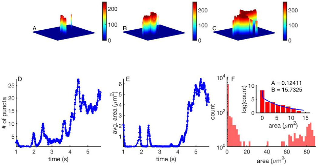
Time evolution of IP₃-induced hierarchical Ca²⁺ signals in a single human cortical neuron. Example image with a Ca²⁺ blip due to the opening of a single IP₃R and a single puff (A), multiple Ca²⁺ puffs interacting to form a bigger event (B), and global Ca²⁺ wave sweeping the entire neuron towards the end of the experiment (C). The number of events (D) increases till a global Ca²⁺ wave ensues as indicated by the mean area/event (E). Histogram of the event sizes (F, main) fitted by a double exponential function having decay constants A1 and A2 to the small events to indicate the existence of blips and puffs (F, inset).

Kinetics of Plasma Membrane Aβ Pores

PunctaSpecks can also detect very small events that typically stay confined to a single pixel, are as short-lived as a single frame, and lead to very small changes in fluorescence intensity. To demonstrate this, we apply PunctaSpecks to the activity of Ca²⁺-permeable pores formed by Aβ42 oligomers in the plasma membrane of Xenopus laevis oocytes. The activity of these pores was recorded using high throughput and massively parallel TIRF microscopy technique called “optical patch clamp” that generates huge imaging records stored in movie files that could be hundreds of Megabytes in size [25]. Processing such a movie file using PunctaSpecks reveals several functional Aβ pores over one second duration of the experiment (see Figure 8A–C for examples). The number of Ca²⁺ influx events into the cytoplasm due to the opening of individual pores (this also represents the number of active pores), mean intensity (fluorescence change per pore), and average area per event (area over which fluorescence increases due to the opening of a single pore) as functions of time are shown in Figure 8D–F. Histograms of the area, dwell times in the open state, and mean open times are shown in Figure 8G–I. In addition to the overall population behavior shown here, a range of statistics about individual pores are also saved by PunctaSpecks (not shown).

Figure 8.

Characterizing the activity of Ca²⁺-permeable pores formed by Aβ42 in the plasma membrane of Xenopus laevis oocytes. Identified individual pores at the start (A), middle (B), and end of the experiment (C). Time evolution of the number of puncta (or active pores) (D), their mean intensity (mean change in fluorescence due to a single opening of a pore) (E), and average area per event (the area over which the fluorescence changes due to an opening of a single pore) (F). Histograms of the spatial size (G), dwell times in open state (H), and mean open times (I).

Discussion and Conclusions

Recent developments in imaging hardware and fluorescent probes for visualizing multiple types of biological processes simultaneously at a wide range of spatiotemporal scales from single biomolecule to whole cell have revolutionized biological research. However, computational tools to process and extract all useful information from the enormous data generated by these high-resolution experiments are lagging behind. In many cases, this has created major bottlenecks in utilizing the full potential of these very powerful experimental techniques. While several programs for specific jobs exist, a comprehensive tool that can extract all key information from the imaging data is still missing. For example, Fiji/ImageJ [36] is a widely used image/movie processing tool with dedicated plugins [32, 64] for specific purposes. Although Fiji can handle the standard processing of imaging data such as noise removal, filtering, and thresholding, there is currently no all-in-one plugin that reports key parameters such as dwell-times, interaction between two biological objects, co-localization and co-occurrence of more than one type of events or objects in multiple image stacks. The ability to calculate these parameters will enable investigators to fully understand the mechanisms underpinning various biological processes as the movement of different proteins can be quantified. In addition to Fiji/ImageJ, there are also CellSpecks [65] and FLICKA [37] that can be used to analyze image stacks. CellSpecks is a Java-based software developed for high throughput analysis of images. While it can analyze large data sets and generate results for thousands of fluorescently labelled fluorophores, it is not capable of tracking mobile objects over time [65]. FLICKA is a Python-based program for analyzing fluorescently labelled objects in individual files but cannot characterize multiple images simultaneously and generate results on more than one type of quantifiable objects. FLICKA is also not able to manage large data sets as the software suffers from speed issues in situations where the activity of fluorophores is extensive, or image stacks contain thousands of objects with tens of thousands of events [37].

To fill the gaps in the existing techniques, we developed an efficient and inclusive tool called PunctaSpecks. PunctaSpecks can process and analyze imaging data from a variety of fluorescence microscopy experiments on the dynamics of a few or hundreds of a single or two different types of biological processes recorded simultaneously in their native environment. PunctaSpecks can extract a wide range of statistics from images carrying information about biological processes at different spatiotemporal scales, ranging from single molecules such as the gating of ion channels to the whole cell signals such as global waves and oscillations. We believe that this tool will facilitate the development of computational models for biological mechanisms based on unprecedented information recorded in the native cell environment.

To demonstrate the utility of PunctaSpecks and verify its accuracy, we initially applied it to synthetic data sets with different signal-to-noise ratios. We then used it to identify biologically relevant information from time-lapse image stacks obtained from different setups, including the interaction of STIM1 and ORAI1 complexes during SOCE, the gating and interaction of IP3R channels giving rise to local and global Ca²⁺ signals in human cortical neurons, and the activity of cation-permeable Aβ pores in the plasma membrane of Xenopus laevis oocytes. PunctaSpecks successfully delineates the relevant information about the biological processes from image stacks and generates CSV files that allow users to import, view, and analyze the data in other software such as Origin, Excel, R, and Python. For tracking purpose, the CSV files for each identified object can be uploaded in Fiji or other software for viewing and further processing.

While PunctaSpecks can process biological data from a wide range of experimental processes under diverse conditions, it has certain limitations. In its current form, it can process imaging data from two different types of biomolecules or biological processes simultaneously. To analyze images carrying information about more than two types of processes, one will have to run PunctaSpecks multiple times, each time extracting information about one or two types of processes and then assembling the CSV files stored during each run for final analysis. Alternatively, users with expertise in MATLAB can extend the open source code included with this paper to handle multiple proteins by copying, pasting, and modifying the routines used for two types of processes. Furthermore, since PunctaSpecks performs pixel-based processing, in its current form it cannot delineate the background “hot spots” present in the system before any stimulus from those that appear in response to stimulation. In the case of STIM1, the software is unable to differentiate between STIM1 moving along the microtubules and STIM1 puncta that appear after stimulating the cell. Therefore, unless the experimental setup provides a distinction between the two different sources of fluorescence (moving of STIM1 along the microtubule and formation of puncta), the software will treat them the same way. Adding such capabilities requires machine learning algorithms that can be incorporated in the future versions of PunctaSpecks as more experimental details emerge about the biological processes investigated. Nevertheless, the first version of PunctaSpecks extracts a wide range of information about the underlying biological processes from fluorescence images with a few easy steps that, to our current knowledge, are beyond the scope of any existing individual tool.

Highlights.

• A comprehensive computational tool for processing and characterizing imaging data from fluorescence microscopy experiments.

• Characterizing imaging data with information about multiple biomolecules or biological processes.

• Calculating the number, areas, life-times, and amplitudes of fluorescence signals arising from multiple sources.

• Tracking diffusing fluorescence sources like moving mitochondria

• Determining the overlap probability of two processes or organelles imaged using indicator dyes of different colors.

• Applying the tool to different data sets recorded under physiological and pathological conditions including synthetic data, interaction of ORAI1 and STIM1, IP₃-induced Ca²⁺ signals in human cortical neurons, and amyloid beta -induced Ca²⁺ influx to the cell.

References

- [1].Alvarez LAJ, Widzgowski B, Ossato G, van den Broek B, Jalink K, Kuschel L, Roberti MJ, Hecht F, SP8 FALCON: a novel concept in fluorescence lifetime imaging enabling video-rate confocal FLIM, Nat Methods, 16 (2019). [Google Scholar]
- [2].Picco A, Mund M, Ries J, Nedelec F, Kaksonen M, Visualizing the functional architecture of the endocytic machinery, Elife, 4 (2015). [DOI] [PMC free article] [PubMed] [Google Scholar]
- [3].Tsien RY, Imagining imaging’s future, Nat Cell Biol, (2003) Ss16–Ss21. [PubMed] [Google Scholar]
- [4].Stephens DJ, Allan VJ, Light microscopy techniques for live cell Imaging, Science, 300 (2003) 82–86. [DOI] [PubMed] [Google Scholar]
- [5].Lippincott-Schwartz J, Patterson GH, Development and use of fluorescent protein markers in living cells, Science, 300 (2003) 87–91. [DOI] [PubMed] [Google Scholar]
- [6].Demuro A, Parker I, Imaging the activity and localization of single voltage-gated Ca2+ channels by total internal reflection fluorescence microscopy, Biophys J, 86 (2004) 3250–3259. [DOI] [PMC free article] [PubMed] [Google Scholar]
- [7].Demuro A, Parker I, Imaging single-channel calcium microdomains by total internal reflection microscopy, Biol Res, 37 (2004) 675–679. [DOI] [PubMed] [Google Scholar]
- [8].Demuro A, Parker I, Optical single-channel recording: imaging Ca2+ flux through individual ion channels with high temporal and spatial resolution, J Biomed Opt, 10 (2005). [DOI] [PubMed] [Google Scholar]
- [9].Work SS, Warshaw DM, Computer-Assisted Tracking of Actin Filament Motility, Anal Biochem, 202 (1992) 275–285. [DOI] [PubMed] [Google Scholar]
- [10].Ghosh RN, Webb WW, Automated Detection and Tracking of Individual and Clustered Cell-Surface Low-Density-Lipoprotein Receptor Molecules, Biophys J, 66 (1994) 1301–1318. [DOI] [PMC free article] [PubMed] [Google Scholar]
- [11].Gelles J, Schnapp BJ, Sheetz MP, Tracking Kinesin-Driven Movements with Nanometre-Scale Precision, Nature, 331 (1988) 450–453. [DOI] [PubMed] [Google Scholar]
- [12].Berridge MJ, Lipp P, Bootman MD, The versatility and universality of calcium signalling, Nature reviews Molecular cell biology, 1 (2000) 11. [DOI] [PubMed] [Google Scholar]
- [13].Islam MS, Calcium signaling, Springer Science & Business Media; 2012. [Google Scholar]
- [14].Takamatsu T, Wier WG, Calcium Waves in Mammalian Heart - Quantification of Origin, Magnitude, Wave-Form, and Velocity, Faseb J, 4 (1990) 1519–1525. [DOI] [PubMed] [Google Scholar]
- [15].Guatimosim S, Guatimosim C, Song LS, Imaging Calcium Sparks in Cardiac Myocytes, Light Microscopy: Methods and Protocols, 689 (2011) 205–214. [DOI] [PMC free article] [PubMed] [Google Scholar]
- [16].Janicek R, Hotka M, Zahradnikova A, Zahradnikova A, Zahradnik I, Quantitative Analysis of Calcium Spikes in Noisy Fluorescent Background, Plos One, 8 (2013). [DOI] [PMC free article] [PubMed] [Google Scholar]
- [17].Tallini YN, Ohkura M, Choi BR, Ji GJ, Imoto K, Doran R, Lee J, Plan P, Wilson J, Xin HB, Sanbe A, Gulick J, Mathai J, Robbins J, Salama G, Nakai J, Kotlikoff MI, Imaging cellular signals in the heart in vivo: Cardiac expression of the high-signal Ca2+ indicator GCaMP2, P Natl Acad Sci USA, 103 (2006) 4753–4758. [DOI] [PMC free article] [PubMed] [Google Scholar]
- [18].Terrar DA, Calcium Signaling in the Heart, Calcium Signaling, Springer; 2020, pp. 395–443. [DOI] [PubMed] [Google Scholar]
- [19].Fearnley CJ, Roderick HL, Bootman MD, Calcium signaling in cardiac myocytes, Cold Spring Harbor perspectives in biology, 3 (2011) a004242. [DOI] [PMC free article] [PubMed] [Google Scholar]
- [20].Arispe N, Pollard HB, Rojas E, Giant multilevel cation channels formed by Alzheimer disease amyloid beta-protein [A beta P-(1-40)] in bilayer membranes, Proc Natl Acad Sci U S A, 90 (1993) 10573–10577. [DOI] [PMC free article] [PubMed] [Google Scholar]
- [21].Demuro A, Smith M, Parker I, Single-channel Ca(2+) imaging implicates Abeta1–42 amyloid pores in Alzheimer’s disease pathology, J Cell Biol, 195 (2011) 515–524. [DOI] [PMC free article] [PubMed] [Google Scholar]
- [22].Lin H, Bhatia R, Lai R, Amyloid beta protein forms ion channels: implications for Alzheimer’s disease pathophysiology, Faseb J, 15 (2001) 2433–2444. [DOI] [PubMed] [Google Scholar]
- [23].Ullah G, Demuro A, Parker I, Pearson JE, Analyzing and Modeling the Kinetics of Amyloid Beta Pores Associated with Alzheimer’s Disease Pathology, Plos One, 10 (2015). [DOI] [PMC free article] [PubMed] [Google Scholar]
- [24].Shah S.l., Demuro A, Mak D-OD, Parker I, Pearson JE, Ullah G, TraceSpecks: a software for automated idealization of noisy patch-clamp and imaging data, Biophys J, 115 (2018) 9–21. [DOI] [PMC free article] [PubMed] [Google Scholar]
- [25].Demuro A, Smith M, Parker I, Single-channel Ca2+ imaging implicates A beta 1–42 amyloid pores in Alzheimer’s disease pathology, J Cell Biol, 195 (2011) 515–524. [DOI] [PMC free article] [PubMed] [Google Scholar]
- [26].Subedi KP, Ong HL, Son GY, Liu XB, Ambudkar IS, STIM2 Induces Activated Conformation of STIM1 to Control Orail Function in ER-PM Junctions, Cell Rep, 23 (2018) 522–534. [DOI] [PubMed] [Google Scholar]
- [27].Ong HL, Ambudkar IS, The endoplasmic reticulum-plasma membrane junction: A hub for agonist regulation of Ca2+ entry, Cold Spring Harbor perspectives in biology, (2019) a035253. [DOI] [PMC free article] [PubMed] [Google Scholar]
- [28].Shin DM, Son A, Park S, Kim MS, Ahuja M, Muallem S, The TRPCs, Orais and STIMs in ER/PM Junctions, Adv Exp Med Biol, 898 (2016) 47–66. [DOI] [PubMed] [Google Scholar]
- [29].Chung WY, Jha A, Ahuja M, Muallem S, Ca2+ influx at the ER/PM junctions, Cell Calcium, 63(2017)29–32. [DOI] [PMC free article] [PubMed] [Google Scholar]
- [30].Meijering E, Smal I, Danuser G, Tracking in molecular bioimaging, leee Signal Proc Mag, 23 (2006) 46–53. [Google Scholar]
- [31].Chenouard N, Smal I, de Chaumont F, Maska M, Sbalzarini IF, Gong YH, Cardinale J, Carthel C, Coraluppi S, Winter M, Cohen AR, Godinez WJ, Rohr K, Kalaidzidis Y, Liang L, Duncan J, Shen HY, Xu YK, Magnusson KEG, Jalden J, Blau HM, Paul-Gilloteaux P, Roudot P, Kervrann C, Waharte F, Tinevez JY, Shorte SL, Willemse J, Celler K, van Wezel GP, Dan HW, Tsai YS, de Solorzano CO, Olivo-Marin JC, Meijering E, Objective comparison of particle tracking methods, Nat Methods, 11 (2014) 281–U247. [DOI] [PMC free article] [PubMed] [Google Scholar]
- [32].Tinevez JY, Perry N, Schindelin J, Hoopes GM, Reynolds GD, Laplantine E, Bednarek SY, Shorte SL, Eliceiri KW, TrackMate: An open and extensible platform for single-particle tracking, Methods, 115 (2017) 80–90. [DOI] [PubMed] [Google Scholar]
- [33].Crocker JC, Grier DG, Methods of digital video microscopy for colloidal studies, J Colloid Interf Sci, 179 (1996) 298–310. [Google Scholar]
- [34].Shah S.l., Smith M, Parker I, Ullah G, Demuro A, CellSpecks: A Software for Automated Detection and Analysis for Calcium Channels in Live Cells, Biophys J, 114 (2018) 291a–291a. [DOI] [PMC free article] [PubMed] [Google Scholar]
- [35].Bruno WJ, Ullah G, Mak D-OD, Pearson JE, Automated maximum likelihood separation of signal from baseline in noisy quantal data, Biophys J, 105 (2013) 68–79. [DOI] [PMC free article] [PubMed] [Google Scholar]
- [36].Schneider CA, Rasband WS, Eliceiri KW, NIH Image to ImageJ: 25 years of image analysis, Nat Methods, 9 (2012) 671–675. [DOI] [PMC free article] [PubMed] [Google Scholar]
- [37].Ellefsen KL, Lock JT, Settle B, Karsten CA, Parker I, Applications of FLIKA, a Python-based image processing and analysis platform, for studying local events of cellular calcium signaling, Bba-Mol Cell Res, 1866 (2019) 1171–1179. [DOI] [PMC free article] [PubMed] [Google Scholar]
- [38].Von Wegner F, Both M, Fink RHA, Automated detection of elementary calcium release events using the A Trous wavelet transform, Biophys J, 90 (2006) 2151–2163. [DOI] [PMC free article] [PubMed] [Google Scholar]
- [39].Rueckl M, Lenzi SC, Moreno-Velasquez L, Parthier D, Schmitz D, Ruediger S, Johenning FW, SamuROI, a Python-Based Software Tool for Visualization and Analysis of Dynamic Time Series Imaging at Multiple Spatial Scales, Front Neuroinform, 11 (2017) 1–14. [DOI] [PMC free article] [PubMed] [Google Scholar]
- [40].Picht E, Zima AV, Blatter LA, Bers DM, SparkMaster: automated calcium spark analysis with ImageJ, American Journal of Physiology-Cell Physiology, 293 (2007) C1073–C1081. [DOI] [PubMed] [Google Scholar]
- [41].Steele EM, Steele DS, Automated detection and analysis of Ca2+ sparks in xy image stacks using a thresholding algorithm implemented within the open-source image analysis platform ImageJ, Biophys J, 106 (2014) 566–576. [DOI] [PMC free article] [PubMed] [Google Scholar]
- [42].Cheng H, Song L-S, Shirokova N, Gonzalez A, Lakatta EG, Rios E, Stern MD, Amplitude distribution of calcium sparks in confocal images: theory and studies with an automatic detection method, Biophys J, 76 (1999) 606–617. [DOI] [PMC free article] [PubMed] [Google Scholar]
- [43].Francis M, Qian X, Charbel C, Ledoux J, Parker JC, Taylor MS, Automated region of interest analysis of dynamic Ca2+ signals in image sequences, American Journal of Physiology Cell Physiology, 303 (2012) C236–C243. [DOI] [PMC free article] [PubMed] [Google Scholar]
- [44].Kong CH, Soeller C, Cannell MB, Increasing sensitivity of Ca2+ spark detection in noisy images by application of a matched-filter object detection algorithm, Biophys J, 95 (2008) 60166024. [DOI] [PMC free article] [PubMed] [Google Scholar]
- [45].Bray M-A, Geisse NA, Parker KK, Multidimensional detection and analysis of Ca2+ sparks in cardiac myocytes, Biophys J, 92 (2007) 4433–4443. [DOI] [PMC free article] [PubMed] [Google Scholar]
- [46].Bányász T, Chen-Izu Y, Balke C, Izu LT, A new approach to the detection and statistical classification of Ca2+ sparks, Biophys J, 92 (2007) 4458–4465. [DOI] [PMC free article] [PubMed] [Google Scholar]
- [47].Wegner F, Both M, Fink R, Automated detection of elementary calcium release events using the à trous wavelet transform, Biophys J, 90 (2006) 2151–2163. [DOI] [PMC free article] [PubMed] [Google Scholar]
- [48].Otsu N, Threshold Selection Method from Gray-Level Histograms, Ieee T Syst Man Cyb, 9 (1979) 62–66. [Google Scholar]
- [49].Smith TG, Marks WB, Lange GD, Sheriff WH, Neale EA, Edge-Detection in Images Using Marr-Hildreth Filtering Techniques, J Neurosci Meth, 26 (1988) 75–81. [DOI] [PubMed] [Google Scholar]
- [50].Marr D, Hildreth E, Theory of Edge-Detection, Proc R Soc Ser B-Bio, 207 (1980) 187–217. [DOI] [PubMed] [Google Scholar]
- [51].Hua G, Akbarzadeh A, A Robust Elastic and Partial Matching Metric for Face Recognition, Ieee I Conf Comp Vis, (2009) 2082–2089. [Google Scholar]
- [52].Olivo-Marin JC, Extraction of spots in biological images using multiscale products, Pattern Recogn, 35 (2002) 1989–1996. [Google Scholar]
- [53].Thomann D, Rines D, Sorger P, Danuser G, Automatic fluorescent tag detection in 3D with super-resolution: Application to the analysis of chromosome movement, Biophys J, 82 (2002) 176a–176a. [DOI] [PubMed] [Google Scholar]
- [54].Ober RJ, Ram S, Ward ES, Localization accuracy in single-molecule microscopy (vol 86, pg 1185, 2004), Biophys J, 87 (2004) 1399–1399. [DOI] [PMC free article] [PubMed] [Google Scholar]
- [55].Manders EMM, Verbeek FJ, Aten JA, Measurement of Colocalization of Objects in DualColor Confocal Images, J Microsc-Oxford, 169 (1993) 375–382. [DOI] [PubMed] [Google Scholar]
- [56].Qian H, Sheetz MP, Elson EL, Single particle tracking. Analysis of diffusion and flow in two-dimensional systems, Biophys J, 60 (1991) 910–921. [DOI] [PMC free article] [PubMed] [Google Scholar]
- [57].Michalet X, Mean square displacement analysis of single-particle trajectories with localization error: Brownian motion in an isotropic medium, Phys Rev E Stat Nonlin Soft Matter Phys, 82 (2010) 041914. [DOI] [PMC free article] [PubMed] [Google Scholar]
- [58].Rueden CT, Schindelin J, Hiner MC, DeZonia BE, Walter AE, Arena ET, Eliceiri KW, ImageJ2: ImageJ for the next generation of scientific image data, Bmc Bioinformatics, 18 (2017). [DOI] [PMC free article] [PubMed] [Google Scholar]
- [59].Deshpande A, Mina E, Glabe C, Busciglio J, Different conformations of amyloid β induce neurotoxicity by distinct mechanisms in human cortical neurons, Journal of Neuroscience, 26 (2006) 6011–6018. [DOI] [PMC free article] [PubMed] [Google Scholar]
- [60].Lock JT, Parker I, Smith IF, A comparison of fluorescent Ca2+ indicators for imaging local Ca2+ signals in cultured cells, Cell calcium, 58 (2015) 638–648. [DOI] [PMC free article] [PubMed] [Google Scholar]
- [61].Fish KN, Total internal reflection fluorescence (TIRF) microscopy, Curr Protoc Cytom, Chapter 12 (2009) Unitl2 18. [DOI] [PMC free article] [PubMed] [Google Scholar]
- [62].Fish KN, Total internal reflection fluorescence (TIRF) microscopy, Current protocols in cytometry, 50 (2009) 12.18. 11–12.18. 13. [DOI] [PMC free article] [PubMed] [Google Scholar]
- [63].Aaron JS, Taylor AB, Chew TL, Image co-localization - co-occurrence versus correlation, J Cell Sci, 131 (2018). [DOI] [PubMed] [Google Scholar]
- [64].Cheezum MK, Walker WF, Guilford WH, Quantitative comparison of algorithms for tracking single fluorescent particles, Biophys J, 81 (2001) 2378–2388. [DOI] [PMC free article] [PubMed] [Google Scholar]
- [65].Sshah S.l., Smith M, Swaminathan D, Psarkser I, Ullah G, Demuro A, CellSpecks: A Software for Automated Detection and Analysis of Calcium Channels in Live Cells, Biophys J, 115 (2018) 2141–2151. [DOI] [PMC free article] [PubMed] [Google Scholar]
Associated Data
This section collects any data citations, data availability statements, or supplementary materials included in this article.