

SUMMARY
Intracellular free calcium concentrations ([Ca2+]i) are assessed by measuring indicator fluorescence in entire cells or subcellular regions using fluorescence microscopy. [Ca2+]i is calculated using equations which link fluorescence intensities (or intensity ratios) to calcium concentrations (Grynkiewicz et al., 1985). However, if calcium ions are heterogeneously distributed within a region of interest, then the observed average fluorescence intensity may not reflect average [Ca2+]i. We assessed potential calcium determination errors in mathematical and experimental models consisting of ‘low’ and ‘high’ calcium compartments, using indicators with different calcium affinity. [Ca2+] calculated using average fluorescence intensity was lower than the actual mean concentrations. Low affinity indicators reported higher (more accurate) values than their high affinity counterparts. To estimate compartment dimensions and respective [Ca2+], we extended the standard approach by using different indicator responses to the same [Ca2+]. While two indicators were sufficient to provide a partial characterization of two-compartment model systems, the use of three or more indicators offered full description of the model provided compartmental [Ca2+] were within the indicator sensitivity ranges. These results show that uneven calcium distribution causes underestimation of actual [Ca2+], and offers novel approaches to estimating calcium heterogeneity.
INTRODUCTION
Ca2+ homeostasis is intensively studied in living cells using ion-sensitive fluorescent indicators, such as fura-2 [1,2]. A quantitative estimate of ion concentrations can be derived from measurements of indicator fluorescence provided that several important experimental conditions are considered [3–5]. For example, the ion-sensitive indicator should be chemically uniform and evenly distributed within the cytosol, indicator binding and fluorescence properties within cells should be similar to those measured in isolated systems, the imaging and measurement system should provide a linear estimate of fluorescence emission, and the free ion concentration should fall within the indicator’s useful dynamic range.
In this paper we examine the hypothesis that significant measurement errors are introduced by the presence of non-uniform distribution of Ca2+ ions. Any imaging system analyzes data within user-identified regions of interest (ROI), which may be as large as an entire field of view, or as small as a single pixel at the optical resolution of the microscope. The observed fluorescence intensity is derived from all of the indicator molecules that contribute signal to the ROI, including areas above and below the focal plane. Even a resolution-limited spot includes signal from a finite region, the shape of which is determined by the three-dimensional point-spread function of the optical system. For example, with laser scanning confocal or two-photon microscopy, the lateral and axial resolutions are estimated at ~0.3 and ~ 1 μm, respectively, with the confocal microscopy offering slightly better resolution [6]. If Ca2+ is distributed uniformly, then the measured average fluorescence intensity (or ratio of average fluorescence intensities, for ratiometric indicators) provides an accurate measure of the average proportion of Ca2+-bound indicator molecules, which in turn can be used to derive estimated [Ca2+]i according to the method of Grynkiewicz and coworkers [1].
How is this relationship affected if Ca2+ is not uniformly distributed within an ROI? Some cellular non-uniformities, such as macrodomains or standing dendritic gradients, are relatively large and can be demonstrated using conventional microscopy (e.g., [7–11]). However, mathematical modeling [12–14] and indirect experiments using kinetically different Ca2+ buffers (BAPTA and EGTA [15–19]) suggest that domains featuring very high Ca2+ concentration may stretch for only 50–150 nm from the channel (for a detailed analysis see [20]). Such small domains can be difficult (e.g., [20–22]) or impossible to image directly (see [23] for review), even under confocal or multiphoton microscopy [6]. Furthermore, the domains might persist in neuronal somata for hundreds of milliseconds [11,24], their properties determined by the presence of buffers [25–28] and diffusion barriers [29–31]. These considerations raise two potential problems for cytosolic ion measurement. First, in any situation where there is spatial heterogeneity in ion concentrations within ROIs, the average fluorescence intensity (or fluorescence ratio) is used to calculate the average Ca2+ concentration. Second, the presence of microdomains with very high [Ca2+]i raises the possibility that indicator molecules may be fully saturated in hot spots, yet appear to be within their dynamic range for the ROI as a whole.
To examine these problems, we assessed the effects of calcium spatial heterogeneity and indicator affinity in computer and in vitro models in which the measured ROI encompasses either a single uniform compartment or two sub-resolution compartments with high and low Ca2+ concentrations. Furthermore, we developed and tested a method to characterize the Ca2+ distribution in such a system using multiple fluorescent indicators.
MATERIALS AND METHODS
Modeling indicator fluorescence and Ca2+ concentration in the presence of a non-uniform Ca2+ distribution.
We consider a hypothetical system composed of two sub-resolution compartments featuring calcium concentrations of [Ca2+]s and [Ca2+]1-s, which are represented in an image as regions with relative dimensions s and 1-s, respectively. The actual mean Ca2+ concentration ([Ca2+] act) in such a system is the weighted average of compartmental Ca2+ concentrations
| (1) |
In either compartment, an indicator would become Ca2+-bound to the extent determined by its affinity for calcium in accordance with the formula
| (2) |
which can be applied to any indicator binding Ca2+ ions with 1:1 stoichiometry as long as the indicator does not significantly reduce the free ion concentration ( e.g. [32]). KD is the indicator apparent dissociation constant and α denotes the fraction of Ca2+-bound indicator. The indicator fluorescence in either compartment can be expressed as
| (3) |
where FB and FF are the fluorescence of Ca2+-bound and Ca2+-free indicator, presumably identical in both compartments. Since both compartments are contained within the same ROI, the collected fluorescence (Fobs) is a linear superposition of indicator fluorescence in both compartments Fs and F1-s
| (4) |
If only the observed averaged fluorescence (Fobs) is available, then overall Ca2+ concentration ([Ca2+]obs) is estimated using the formula
| (5) |
which may be compared to the actual mean Ca2+ concentration calculated using Eq. 1.
Determination of Ca2+ distribution in a steady-state submembrane domain
We considered a submicroscopic domain surrounding a single point source of Ca2+ entry, such as an L-type voltage gated channel, in a hemispherical space. In the presence of moderate buffer concentrations, calcium distribution around the pore can be described using the rapid buffer approximation [33], an approach offering an explicit linear solution for a single mobile buffer [34]. Using this approach, we calculated [Ca2+] in the distance r from an open channel
| (6) |
where
| (7) |
assuming that the channel passed Ca2+ current (σ) of 0.5 pA, bulk cytosolic Ca2+ concentration (c∞) was 0.1 μM, diffusion coefficients of Ca2+ (DCA) and mobile buffer (DBUF) were 250 and 75 μm2/s, respectively, and the system contained 250 μM Ca2+ buffer ([BUF]T) with apparent dissociation constants (KB) of 1 μM [17,34,35].
Determination of indicator fluorescence in a two-compartment model system.
We built an in vitro model system consisting of two microslides with 20 μm interior depth (Vitrocom, Mountain Lakes, NJ) intersecting at a 90° angle (see inset in Fig. 2A). The microslides were filled with calibration buffers (pH=7.20) containing 100 mM KCl, 10 mM MOPS, 10 mM EGTA and different free Ca2+ concentrations prepared by mixing 10 mM EGTA and 10 mM Ca-EGTA standard buffers (Molecular Probes, Eugene, OR) and 50 μM of the following Ca2+ indicators: fura-2 (KD=0.22 μM; [1]), fura-5F (KD =0.4 μM; [36]), fura-4F (KD =0.77 μM; [36]), fura-6F (KD =5.3 μM; [36]) (Molecular Probes, Eugene, OR), and fura-2FF (KD =6 μM; [37]) (TefLabs, Austin TX). The accuracy of solution preparation and free Ca2+ concentration in the absence of indicators was verified with a Ca2+ selective electrode (Ionplus 97–20, Orion Res., Beverly, MA) previously calibrated against a series of calibration buffers.
Fig. 2. Calcium concentrations reported by indicators featuring different affinities for calcium in two-compartment in vitro systems.
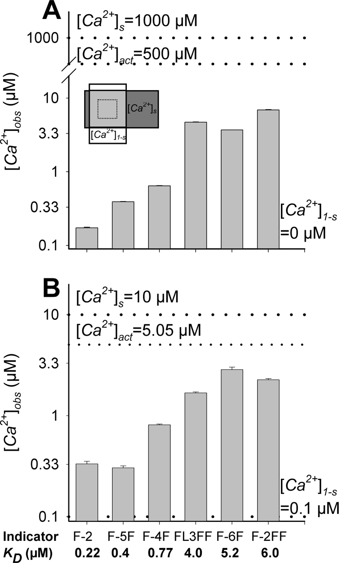
We measured the average fluorescence intensity in a system consisting of two overlapping 20 μm thick microslides (s=0.5) (A, inset) containing 0 and 1 mM free calcium (A) or, nominally, 0.1 and 10 μM (B) free calcium. Upon collecting the fluorescence of several indicators (fura-2 (F-2), fura-5F (F-5F), fura-4F (F-4F), fluo-3FF (FL3FF), fura-6F (F-6F) and fura-2FF (F2FF) from the ROI (A, inset, dashed box), we calculated [Ca2+]obs using Eq. 8 and 9 [1] as if the fluorescence were collected from a uniform system. As a reference, we marked the nominal free calcium concentrations in both compartments and their average (dotted lines). The data were derived from 2–4 independent experiments.
The microslides were visualized through a 530 nm emission filter with a cooled CCD camera (Cooke, Auburn Hills, MI) on a Nikon Eclipse TE300 inverted microscope with 20x/0.45 Plan Fluor lens (Nikon Inc., Melville, NY). Images were collected at alternate illumination wavelengths (340/380 nm; 75 W xenon arc lamp) and, after subtracting the matching wavelength background, divided by one another to yield ratio images. For simultaneous measurements, we filled the microslides with buffers containing 50 μM fura-2 and fluo-3FF (KD=4 μM; Hyrc-unpublished observation) and collected indicator fluorescence excited at the respective excitation wavelengths: 340/380 nm (fura-2) and 485 nm (fluo-3FF).
During an offline analysis, we defined the regions of interest (ROI) within the cross section of overlapping microslides (~50 by 50 μm), determined the average fluorescence (Fobs) or ratio (Robs) values, and used the formulas [1]
| (8) |
| (9) |
to calculate free calcium concentrations ([Ca2+]obs) reported by ratiometric and single wavelength indicators, respectively. Fobs and Robs were the measured fluorescence intensity and fluorescence intensity ratio. The symbols FF and FB denoted the fluorescence intensities and RF and RB were ratios of fluorescence intensity excited at 340 and 380 nm of free and Ca2+-bound indicator. F2F/F2B was the correction factor defined as the second wavelength intensity of free and Ca2+-bound indicator [1]. The calibration constants were determined in calibration solutions containing either 10 mM EGTA or 1 mM Ca2+ in the same optical system. The MetaFluor software (Molecular Devices, Sunnyvale, CA) was used for image acquisition and analysis.
Calculating the fractions of Ca2+-bound indicators
The fractions of calcium-bound indicators (αobs) were derived from the indicator fluorescence based on the fact that the observed fluorescence (Fobs) is a linear superposition of free and Ca2+-bound indicator fluorescence FF and FB [1]
| (10) |
This equation readily converts to
| (11) |
a formula allowing αobs determination for single wavelength indicators. Similarly, solving the equation set for fluorescence intensity F1 and F2 excited at two different wavelengths
| (12) |
yields an expression
| (13) |
which is readily simplified into more convenient form
| (14) |
where Robs is the fluorescence intensity ratio, RB and RF are the fluorescence ratios of Ca2+-bound and Ca2+-free indicator, respectively, and β, the correction factor, defined as the ratio of Ca2+-free and Ca2+-bound indicator at the second excitation wavelength (F2F/F2B). The calibration constants were determined in microslides containing 10 mM EGTA or 1 mM free Ca2+.
Calculating the compartmental and average calcium concentrations in the model systems with the use of multiple calcium indicators.
After converting experimentally determined indicator fluorescence and fluorescence intensity ratios into fractions of Ca2+-bound indicators as described above, we split them into components attributable to each compartment using a method described in the Appendix. We used three different strategies to solve the relevant equation system (Eq. A7) and determine the compartment sizes and the fractions of Ca2+-bound indicator in each compartment ( and ). The simplified approach took advantage of the fact that if the relative compartment sizes were known, two indicators would be sufficient to determine the compartmental Ca2+ concentrations. Acting as if s were not known (in the model system s is defined by the ratio of microslide thickness and equal to 0.5), we used the simultaneously determined fluorescence of fura-2 and fluo-3FF to determine the range of s values for which the fractions of Ca2+-bound indicators in both compartments adopted acceptable values (0≤α≤1). The exact method relied on numerical solutions of Eq. A7 with the use of sequentially determined fluorescence of any three indicators. To accommodate data from more than three indicators, we performed the regression analysis of the relationship between the observed fractions of Ca2+-bound indicators and indicator affinities for Ca2+. Using the ‘least-square-method’, we determined and values for which the sum of the squared differences between the experimental and predicted values was minimal. Once the compartment size and fractions of Ca2+-bound i-th indicator were determined, we calculated free calcium concentration in either compartment ([Ca2+]n) using the formula
| (15) |
and the estimated free calcium concentration in the entire system using Eq. 1. The 95% confidence bounds were derived from the Monte Carlo simulations [38]. All calculations were performed using Calculation Center (Wolfram Research, Champaign, IL). SigmaPlot (Systat, Point Richmond, CA) was used to prepare the graphs.
Comparing models using Akaike’s Information Criterion
The relative likelihood of the models to be correct was determined by calculating the evidence ratio defined as 1/e(−0.5*ΔAICc), where ΔAICc is the difference between the second order (corrected) Akaike’s information Criterion (AICc) of models being compared. AICc values for each model were calculated following the formula
| (16) |
where K is the number of data points, L denotes the number of parameters fit by the regression plus one and SS is the sum of squares of vertical distances of the point from the regression line [38].
RESULTS
Simulating indicator fluorescence and calcium concentrations in systems featuring a non-uniform calcium distribution.
In a uniform environment, such as a calibration buffer, the relationship between any single fluorescence intensity or fluorescence intensity ratio of an indicator and corresponding Ca2+ concentration is defined by equations derived by Grynkiewicz and coworkers [1]. The applicability of these equations to systems featuring non-uniform Ca2+ distribution depends on the ability to distinguish local fluorescence intensities. If the areas featuring different calcium concentration, and therefore indicator fluorescence (Fn), were clearly defined, the local Ca2+ concentration in each region ([Ca2+]n) could be determined and the average Ca2+ concentration ([Ca2+]act) in the system consisting of N distinct compartments each featuring an area of sn (Σsn=1) would be a mean of local Ca2+ concentrations
| (17) |
If, however, the calcium domains were smaller than the measured region of interest (ROI), then single fluorescence intensities would remain unresolved. The net fluorescence of the ROI (Fobs) would then represent a spatially averaged value corresponding to several unknown Ca2+ concentrations. Since more detailed information would not be available due to theoretical or practical limitations, the observed fluorescence would subsequently be converted into a single Ca2+ concentration ([Ca2+]obs). In this case, the calculation will follow the formula
| (18) |
It is worth noticing that the actual (Eq. 17) and observed Ca2+ (Eq.18) concentrations are calculated in different ways. While the former is a result of step-by-step averaging of local calcium concentrations derived from local fluorescence intensities, the latter relies on a one step conversion of previously averaged fluorescence. To compare these approaches, we considered a simple model consisting of two sub-resolution compartments with high and low calcium concentrations, with relative sizes of s and 1-s. Calcium concentrations in each compartment were set at levels which might be typical for resting ([Ca2+]1-s=0.1 μM) and stimulated ([Ca2+]s=10 μM) neurons (Fig. 1B). As a reference, we used a system containing the same average concentration of free Ca2+ ions, but distributed evenly throughout the ROI (Fig. 1A). We probed both models with hypothetical high (KD=0.22 μM) and low affinity (KD=6 μM) single wavelength indicators whose behavior in either compartment could be described by the Grynkiewicz equation [1]. For convenience, we assumed our indicators to be non-fluorescent (FF=0) until Ca2+-bound (FB=1), thus making their fluorescence intensity numerically equivalent to the fraction of Ca2+-bound indicator. Assuming further that the indicators were evenly distributed, we simulated the average indicator fluorescence that could be collected from such a system featuring different degrees of heterogeneity (0≤s≤1) (Fig. 1C and D). At the extreme situation where the system consisted of either compartment (s=0 or s=1), a situation equivalent to our uniform reference system (Fig. 1A), the fluorescence and hence, the fractions of Ca2+-bound indicators, depended exclusively on the indicator KD and Ca2+ concentration (Fig. 1C, D). Therefore, the indicator fluorescence could, in principle, be converted into the actual Ca2+ concentrations (Fig. 1E). In practice this may be problematic, as some Ca2+ concentrations may lie beyond the indicator sensitivity range. In particular, the high affinity indicator would be almost completely saturated (Fig. 1C; α~0.98) in the ‘high’ calcium compartment while the low affinity one would remain mostly Ca2+ free in the ‘low’ calcium segment (α~0.04) (Fig. 1D).
Fig. 1. Simulation of indicator fluorescence (C, D) and Ca2+ concentration determination (E) in uniform (A) or non-uniform (B) model systems.
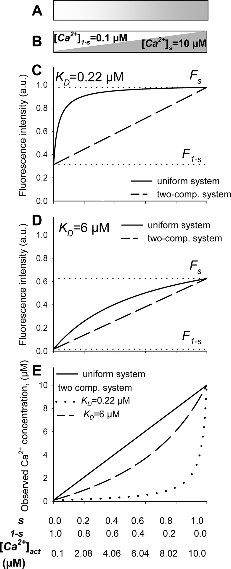
Graphs simulate two systems with average calcium concentration ([Ca2+]act) ranging from 0.1 to 10 μM, that was either evenly distributed (A) or split into two discrete compartments (B). The two-compartment system consisted of ‘high’ ([Ca2+]s = 10 μM) and ‘low’ ([Ca2+]1-s = 0.1 μM) calcium segments having relative dimensions of s and 1-s, respectively. Both systems were probed with two hypothetical indicators featuring calcium affinities corresponding to those of commonly used indicators fura-2 and fura-2FF (KD=0.22 μM and 6 μM, respectively) but offering the same fluorescence change after Ca2+ binding (FF=0 and FB=1). Graphs C and D present the fluorescence of high (C) or low (D) affinity indicators in the uniform system (solid lines), the ‘low’ (F1-s) and ‘high’ (Fs) calcium compartments (C and D; dotted lines) and their linear superposition representing the average fluorescence (Fobs) that would be collected from the non-uniform system (C and D, dashed lines). In E, the Grynkiewicz equation [1] was used to convert the average fluorescence of both indicators into the average calcium concentrations in the uniform (solid line) and the two-compartment (dashed and dotted line) systems.
This situation was radically changed in a non-uniform system (0<s<1) in which indicator from both compartments contributed to the overall fluorescence defined as a weighted average of compartmental fluorescence intensities. Increasing the relative size of the ‘high’ calcium compartment and, therefore the average calcium concentration, led to a linear fluorescence rise from the level in the ‘low’ to that in the ‘high’ calcium compartment (Fig. 1C and D, dashed lines). Interestingly, the mean fluorescence in a two-segment system was lower than that in a uniform system featuring the same average calcium concentrations (Fig. 1C and D, solid lines). This difference was especially large if the system containing a small proportion of the ‘high’ calcium compartment (0.1<s<0.2) and, therefore, a moderate Ca2+ concentration (1 μM<[Ca2+]act<2 μM) was probed with a high affinity indicator (Fig. 1C).
Consequently, converting the average fluorescence from anon-uniform system into Ca2+ concentration using Grynkiewicz equation [1], as if it was collected from a uniform system, produced values (Fig. 1E, dotted and dashed lines) lower than the [Ca2+]act (Fig. 1E, solid lines). The magnitude of this difference depended on both the relative size of the compartments and the affinity of the indicator used. While the [Ca2+]obs derived from the average fluorescence of high affinity indicator did not exceed 15% of the actual concentration as long as either compartment constituted a significant proportion of the system (0.1<s<0.8), the [Ca2+]obs reported by low affinity indicator corresponded to at least ~45% of [Ca2+]act (Fig. 1E). Analogous simulations performed using ratiometric indicators produced identical results (data not shown) suggesting that the relative accuracy of an indicator depends on its binding, rather than spectral, properties.
The above simulations showed that the mean Ca2+ concentrations derived from the average fluorescence or fluorescence intensity ratio collected from a system featuring non-uniform calcium distribution might be lower than the actual ones (for the formal analysis see S1). In such a situation, the low affinity indicators provided higher (more accurate) estimates of the average Ca2+ concentrations than their high affinity analogues (for the formal proofs see S2 and S3). Lastly, the data imply that whenever low affinity indicators report higher Ca2+ concentration than their high affinity analogues, the system might feature a non-uniform Ca2+ distribution.
Average calcium concentration in non-uniform system determined using single indicators.
To illustrate this problem, we built a two-compartment model system consisting of two 20 μm thick microslides (s=0.5) intersecting at a 90° angle (Fig. 2A, inset) filled with buffers of known calcium concentrations. We determined the fluorescence of several indicators (0.22 μM ≤KD≤ 6 μM) in overlapping microslides (our ROI measuring approximately 50 by 50 μm) and calculated [Ca2+]obs using Eq. 8 and 9 [1]. These systems mimic a situation encountered in intracellular free Ca2+ concentration measurements whenever the selected ROI, as large as a cell or as small as single pixel, encompasses regions featuring distinct Ca2+ concentrations.
At first, we examined the system containing Ca2+-free indicator in the ‘low’ Ca2+ compartment ([Ca2+]1-s=0, α1-s=0) and fully Ca2+-bound dye in the ‘high’ calcium compartment ([Ca2+]s=1000 μM, α s ≈1) (Fig. 2A). The fluorescence gathered from the overlapping microslides corresponded to indicators being approximately half Ca2+-bound (0.44≤αobs≤0.52) irrespective of the indicator affinity. While this was correct (αobs =s*αs+(1-s)* α1-s =0.5*1+(1–0.5)*0=0.5), treating fluorescence as if coming from a uniform system produced Ca2+ concentrations corresponding to the KD of each indicator (Fig. 2A). This simple, albeit somewhat extreme, example revealed some critical problems associated with converting average fluorescence from a heterogeneous system into calcium concentration. First, the collected fluorescence was relatively low, suggesting that the measured Ca2+ concentrations lay perfectly within the indicator sensitivity range, while in fact 50% of the indicator was fully saturated. Second, the calculated concentration had surprisingly little in common with the actual calcium levels. While the former ([Ca2+]obs) were roughly equal to the indicator dissociation constant, the latter ([Ca2+]act) could not even be determined as the indicators were saturated in the ‘high’ calcium compartment (αs=1) and unable to report any meaningful concentrations ([Ca2+]s →∞). Third, since the [Ca2+]obs were approximately equal to indicator affinity for calcium, low affinity indicators reported higher [Ca2+]obs than their high affinity counterparts (Fig. 2A), perhaps the only indication that the system featured non-uniform Ca2+ distribution.
Next, we analyzed a somewhat more realistic system consisting of microslides filled with buffers nominally containing 0.1 μM and 10 μM free Ca2+, concentrations equal to those used for modeling purposes (Fig. 1). The indicators (50 μM) reduced the actual [Ca2+]s to values between 7.6 μM (fura-2) and 8.4 μM (fura-2FF) but had practically no effect on [Ca2+]1-s. The [Ca2+]obs determined in this model system were lower than the actual mean calcium concentrations (3.84 μM ≤[Ca2+]act ≤4.25 μM), with lower affinity indicators (KD>1 μM) reporting higher [Ca2+]obs than their high affinity (KD<1 μM) analogues (Fig. 2B). In particular, fura-2 reported [Ca2+]obs equal to 0.33 μM, merely 8.6% of the actual value, whereas its low affinity derivatives, fura-6F and fura-2FF, yielded [Ca2+]obs of ~2.5 μM corresponding to ~59% of the actual value (Tab. 1), a relation predicted by our theoretical considerations (Fig. 1E). Interestingly, in the analyzed system fluorescence averaging led to much bigger [Ca2+]act underestimation than ignoring the buffering capacity of the indicator (Fig. 2B, Tab. 1).
Table 1.
Comparison of the actual, observed and estimated free calcium concentrations in a two-compartment model system.
| Free calcium concentration (μM) | Estimation method¶ | |||||
|---|---|---|---|---|---|---|
| Nominal* | Actual† | Observed‡ | Simplified | Exact | Regression | |
| [Ca2+]s | 10 | 7.6–8.4†† | N/A | ≥3.5§ | 17±7‖ | 5.2≤9.3≤33** |
| [Ca2+]1-s | 0.1 | 0.1 | N/A | ≤0.18 | 0.07±0.03 | 0.0≤0.07≤0.19 |
| s | 0.5 | 0.5 | N/A | 0.26≤s≤0.65 | 0.38±0.03 | 0.48≤0.56≤0.62 |
| [Ca2+] | 5.05 | 3.85–4.25†† | 0.33–2.5‡‡ | ≥2.2 | 5.6±2.0 | 2.8≤6.0≤20 |
- values in buffers in the absence of the indicators,
- concentrations in the presence of 50 μM indicators
- free calcium concentration ([Ca2+]obs) calculated directly from the indicator fluorescence collected from the two-compartment model system using Eq 8 or Eq. 9 as if the system was uniform,
– free calcium concentrations and compartment sizes were derived from multiple indicator data using procedures described the method section,
– minimal and maximal values were calculated (Fig. 3)
– mean ± SEM
- mean and 95% confidence intervals
-the limiting values defined by [Ca2+] in the presence of 50 μM indicators featuring the highest (KD=0.22 μM) and lowest affinity for calcium (KD =6 μM).
– the range of concentrations reported by indicators featuring different affinities for calcium (0.22≤KD≤6 μM) (Fig. 2).
Average calcium concentration in non-uniform system estimated using multiple indicators.
Since single indicators were not able to accurately report average Ca2+ concentrations in our two-compartment systems (Fig. 2, Tab. 1), we sought solutions to this problem using multiple indicators, a notion based on the fact that indicators bind calcium and change their fluorescence to the extent defined by their dissociation constants. To test this approach, we used our mathematical model (Eq. A7) to split indicator fluorescence (Fobs) into components, Fs and F1-s, attributable to either compartment. In all cases, we assumed that the indicator was evenly distributed between the compartments, a condition met by keeping the same indicator concentrations in both capillaries, and that the Grynkiewicz equation [1] described indicator behavior in either compartment. In addition, fluorescence of all indicators reflected the same Ca2+ distribution as required by the model.
At first, we determined concomitantly the fluorescence of fura-2 (KD =0.22 μM) and fluo-3FF (KD=4 μM), indicators that could be imaged simultaneously due to distinct spectral properties. Although these experiments did not provide enough information to fully describe our model system (see the method section for details), the collected data were sufficient to identify the range of possible fractions of Ca2+-bound indicators (0≤α≤1) and the relative areas of the ‘high’ calcium compartment (0≤s≤1) (Fig. 3A and B). This simplified method applied to the system containing 0 and 1 mM free Ca2+ in the ‘low’ and ‘high’ calcium compartments yielded a very limited set of s values (0.44≤s≤0.47, Fig. 3A, hatched box). Under these conditions, both indicators were characterized as mostly Ca2+-free (0≤α≤0.035) in one compartment, while being almost completely bound in the other (0.995≤α≤1), a reasonably accurate description of our model system (Fig. 3A, vertical dashed line). The situation was different in the other system ([Ca2+]1-s =0.1 μM and [Ca2+]s=10 μM) where the relative size of the ‘high’ calcium compartment was defined rather broadly (0.26<s<0.65, Fig. 3B, hatched box). In consequence, the possible fractions of Ca2+-bound indicators (Fig. 3B) and Ca2+ concentration in the ‘low’ (≤0.18 μM) and ‘high’ (≥3.5 μM) calcium compartments could adopt many different values. While these ranges included the actual value (Fig. 3B, vertical dashed line), it was not clear how to determine it more precisely. Furthermore, this method did not allow the determination of the maximum [Ca2+] due to indicator saturation, and so it could not be used to determine the average calcium concentration in the whole system. Taken together these data suggest that the use of two indicators can provide only a partial characterization of the tested model systems (Tab.1) with varying levels of accuracy.
Fig. 3. Partial characterization of a two-compartment system by simultaneous use of two indicators featuring different affinities for calcium and distinct spectral properties.

We determined simultaneously the fluorescence of fura-2 and fluo-3FF in overlapping capillaries (Fig. 2A, inset) filled with buffers containing either 0 and 1 mM (A) or 0.1 and 10 μM (B) free calcium. The indicators (50 μM) had little effect on [Ca2+]1-s but reduced [Ca2+]s, from 10.0 μM (nominal) to 6.55 μM (actual). The physically possible fractions of Ca2+-bound indicators (0≤α≤1) were then plotted against the size of the high calcium compartment (0≤s≤1) to identify the range of s values that would allow coexistence of both compartments (hatched boxes). The vertical dashed lines represent the actual size of the ‘high’ calcium compartment. The presented data were derived from representative experiments.
To determine the calcium concentrations more precisely, we numerically solved the appropriate equation system (Eq. A7), an approach requiring fluorescence data of three indicators. Due to limited spectral resolution and increased Ca2+ buffering, we analyzed the data collected sequentially (Fig. 2), an equivalent approach as long as the system did not change between measurements. Having fluorescence data for six indicators (Fig. 2) while only three were needed, we tested the ability of the exact method to produce valid results by solving the equation system for all unique data subsets. We found that only five out of twenty possible indicator combinations provided meaningful solutions (0≤s≤1 and 0≤α≤1) while the others, probably due to measurement errors, produced results beyond the physically acceptable range (0>s>1 or 0>α>1). Among the latter were sets that included only high (KD≤1 μM) or low (KD ≥ 1 μM) affinity indicators and their combinations. The parameters derived by averaging the relevant data (s= 0.38 ± 0.03, [Ca2+]1-s =0.07 ± 0.03 μM, [Ca2+]s =17 ± 7 μM, and [Ca2+]est=5.6 ± 2.0 μM, Tab.1) were not statistically different from the actual values, a marked improvement over the simplified method (Tab. 1). However, their confidence bounds were rather broad and there was no way to decide a priori which indicators would provide valid results. Therefore, the use of just three indicators, albeit theoretically sufficient to describe a two-compartment system, may not be good enough for the analysis of ‘noisy’ experimental data.
To account for data variability, we fitted our model to all experimental data (Fig. 2). This regression procedure retraced (Fig. 4A and B, solid lines) the experimentally determined fractions of Ca2+-bound indicators (Fig. 4A and B, filled circles) and split them into components attributable to the ‘low’ (α1-s; dashed lines) and the ‘high’ (αs; dotted lines) Ca2+ compartments. In the system containing 0 or 1 mM free calcium, indicators were characterized as either free (α1-s~0) or Ca2+-bound (αs~1) irrespective of indicator KD (Fig. 4A). In contrast, in the presence of moderate Ca2+ concentrations (0.1 and 10 μM) the fractions of Ca2+-bound indicators were found to be inversely related to indicator KD values reflecting weaker ion binding by low affinity indicators (Fig. 4B). In both cases, the indicator behavior (Fig. 4A and B) was consistent with that expected under given circumstances.
Fig. 4. Full description of a two-compartment system with regression analysis of multiple indicator data.
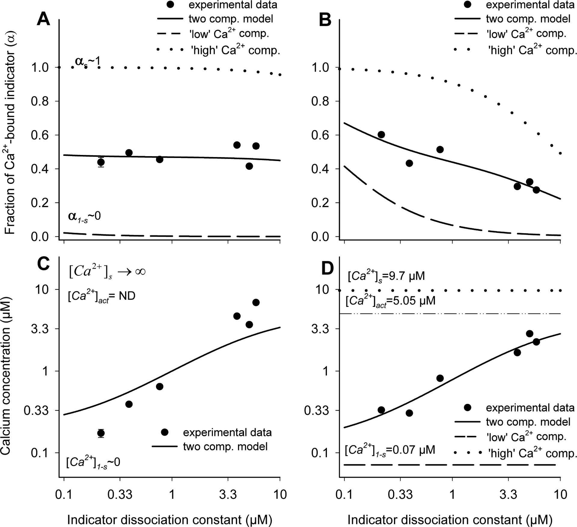
We determined the fluorescence of several indicators (Fig. 2) in two-compartment systems containing either 0 and 1 mM (A) or 0.1 and 10 μM (B) free calcium. The fluorescence data were converted into estimated fractions of Ca2+-bound indicators (αobs) and plotted against indicator KD (A and B). The two-compartment model (A and B; solid lines) was then fitted to experimental data (filled circles) to determine the relative compartment sizes and split the αobs into components attributable to the ‘low’ (dashed line) and ‘high’ (dotted lines) Ca2+ compartments. The results produced by regression analysis (A and B) were subsequently converted into the Ca2+ concentrations (C and D). In one of the systems, the indicator was characterized as fully saturated (A, αs~1) and the [Ca2+]s and [Ca2+]est could not be determined (C; [Ca2+]est =ND).
In the system containing either free or fully Ca2+-bound indicator ([Ca2+]1-s=0 and [Ca2+]s =1 mM), the Ca2+ concentration in the ‘high’ Ca2+ compartment, and therefore the average concentration, could not be determined (Fig. 4C). While this might look like a shortcoming of the method, it actually reflected the fact that fluorescence of almost fully Ca2+-bound indicator (α→1) could not be converted into Ca2+ concentration ([Ca2+]=KD* α /(1-α)→∞), a fundamental limit of indicator applicability. In contrast, as long as the indicators were not saturated, the estimated concentrations (0.07 μM and 9.7 μM in the “low’ and ‘high’ Ca2+ compartments, respectively; Tab. 1) matched the actual values ([Ca2+]1-s=0.1 and [Ca2+]s=10 μM) rather well (Fig. 4D). While the regression and exact methods produced similar results (Tab. 1), the former was clearly superior to the latter, as it could accommodate data from practically unlimited number of indicators and account for their variability.
Taken together these data clearly indicate that the use of three or more indicators could provide a realistic description of a two-compartment model system that cannot be otherwise achieved by the use of any single indicator species (Tab. 1). Since the method is in principle quite general, it might be used to characterize more complex systems.
Modeling calcium concentration within a steady-state microdomain
To examine this problem further, we simulated Ca2+ distribution in a submembrane Ca2+ domain created by Ca2+ influx through an open ion channel using the rapid buffer approximation [33], an approach that was shown to produce excellent results in the presence of moderate concentrations of kinetically fast buffers [35]. The balance between Ca2+ influx, diffusion and binding by an intrinsic buffer results in a steep decline in local Ca2+ concentration from >150 μM in the immediate vicinity of the channel to ~1 μM level just 0.1 μm from the pore (Fig. 5A; solid line). If the indicator fluorescence at each point could be collected, then the local and average Ca2+ concentrations would be known. As this is not the case, the accuracy of the [Ca2+] determination is critically dependent on the spatial resolution of the data collection, the indicator affinity (S4), and the way the data are interpreted (Fig. 5).
Fig. 5. Simulation of indicator fluorescence and free calcium concentration in a steady-state calcium domain.
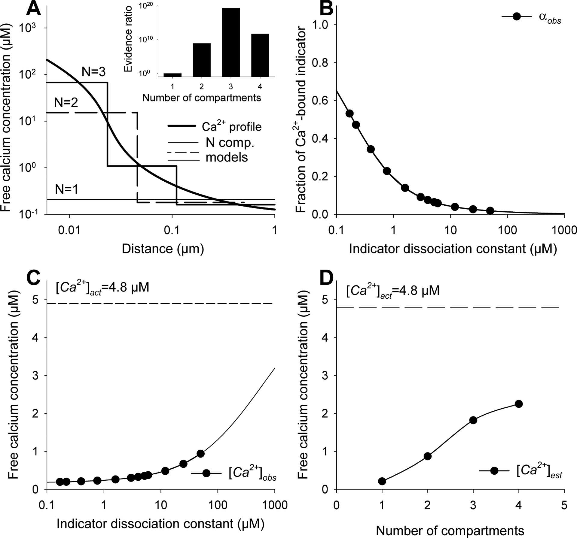
The Ca2+ profile near an open ion channel (A, solid black line) was determined using an analytical steady state solution to the rapid buffer approximation [34] over a distance of 0.001 to 1 μm assuming that the calcium current was 0.5 pA and concentration of intrinsic buffer featuring KB of 1 μM was 250 μM. Calcium and buffer dissociation constants were 250 μm2/s and 75 μm2/s, respectively [17,34]. The Ca2+ concentration far from the pore was 0.1 μM. To be consistent with the basic assumptions of Grynkiewicz model [1], we assumed that the indicator was present in minimal concentrations and did not affect free calcium distribution within the domain. We then calculated the average fluorescence of twelve indicators featuring different affinities for calcium (0.17 μM≤KD≤ 50 μM) that could be collected from the domain (B) and related calcium concentrations (C; [Ca2+]obs). Using the regression method, we created single and multi-compartment representations (A) of the actual free calcium distribution (A, black solid line). The relative likelihood of models being correct was determined by comparing them to a single compartment (uniform) representation using AIC method (A, inset). Finally, the average free calcium concentration within the domain was estimated as a weighted average of compartmental calcium concentrations inferred from different models (D).
If the domain was a uniform, single compartment entity one indicator would be sufficient to estimate the average calcium concentration. As expected, however, [Ca2+]obs determined in this manner depended on the affinity of the indicator (Fig. 5C, S4) and only a very low affinity indicator (KD>1000 μM) would be able to provide a reasonably accurate [Ca2+]act estimate (Fig. 5C). Alternatively, the regression method estimated the mean Ca2+ concentration in one compartment model as equal to ~0.21 μM, merely 5% of the actual value (Fig. 5A).
In contrast, representing the domain as consisting of just two compartments (Fig. 5A, dashed line) not only provided a better estimate of the [Ca2+]act (~1 μM) than a single compartment model (Fig. 5D) but also offered a rough approximation of calcium concentration within (~15 μM) and outside of (~0.2 μM) the domain. Depicting the domain as consisting of three or four compartments produced increasingly better estimates of both local (Fig. 5A) and average (Fig. 5D) Ca2+ concentrations. It is also clear that the multi-compartment models fit the data better than their single compartment analogue (Fig. 5A, inset). However, as we considered only a set of twelve indicators, creating models consisting of four or more compartments becomes difficult as the number of parameters inferred from the regression approaches the number of available data.
Although the number of required indicators restricts for any practical purposes the number of considered compartments, the indicators used for analysis do not need to feature extremely low affinities for calcium to produce realistic results (Fig.5C). For instance, a four-compartment model based on commonly used indicators (0.17 μM≤KD ≤50 μM ) provided the same [Ca2+]act estimate in the domain (2.1 μM, Fig. 5D) as a single low affinity indicator (KD~320 μM) (Fig. 5C). Furthermore, describing the domain as a multi-compartment rather than a uniform entity provides an insight into the calcium distribution within the domain, information that cannot be derived from a single indicator measurement.
DISCUSSION
Single indicators underreport average Ca2+ concentrations in the presence of non-uniform calcium distribution.
Although equations derived by Grynkiewicz and coworkers [1] make no provision for non-uniformity of Ca2+ distribution, they are extensively used to determine the cytosolic free calcium concentrations in cells where the local Ca2+ levels, and therefore the local fluorescence intensities, may be strikingly different. The potential heterogeneity of Ca2+ distribution would not be a problem if the indicator fluorescence corresponding to local Ca2+ concentrations were resolved and individually converted into Ca2+ concentrations on a pixel-by pixel basis (S4). Determining [Ca2+]i in this manner, however, would not be possible if the dimensions of the Ca2+ domains, which might be as small as 0.05–0.1 μm [20], were below the limits of lateral and axial resolution of confocal and two-photon microscopes estimated at ~0.3 μm and ~1 μm, respectively [6]. Alternatively, the problem may occur if the fluorescence intensities of several pixels were averaged to increase the signal-to-noise ratio. While the recently developed methods of imaging Ca2+ influx through single channels, an approach requiring combined use of imaging and electrophysiological techniques and mathematical modeling [39–43], addressed to certain extent the resolution limit problem, most of standard [Ca2+]i measurements is still performed using wide field microscopy and pixel intensity averaging. In either case, the collected fluorescence would represent an average of intensities corresponding to different [Ca2+] and its use to determine [Ca2+] would produce valid results only if Grynkiewicz equations [1] were able to convert average fluorescence into the mean Ca2+ concentration.
To test validity of this critical, yet tacit, assumption, we considered the average indicator fluorescence and mean Ca2+ concentration in a two-compartment model system with known compartmental Ca2+ concentrations (Fig. 1, 2) and a steady-state microdomain described using the rapid buffer approximation method [34]. The simulation (Fig. 1, 5, S4, S5) and experimental data (Fig. 2) demonstrated that Ca2+ concentrations inferred from the average indicator fluorescence or intensity ratio ([Ca2+]obs) using Grynkiewicz equations [1] were lower than the actual ones ([Ca2+]act) even if the observed system was only marginally heterogeneous with respect to free Ca2+ ion distribution (Fig. 1), an observation generalized by a formal analysis (S1–S3). The gap between the [Ca2+]obs and [Ca2+]act was found to depend on both the degree of system heterogeneity and the affinity of the indicator used (Fig. 1, 2, 5, S1–S3). Since the former was somewhat arbitrarily chosen and would not be known in any real system, we focused on the indicator affinity, a property well characterized in buffer systems [2] that can be changed by selecting a different indicator. We found both in theory (Fig. 1, 5, S1–S3) and through experiment (Fig. 2) that the low affinity indicators yielded higher and more accurate estimates of the average Ca2+ concentrations than their high affinity analogues. These results suggest that if low affinity indicators report higher [Ca2+]obs than the high affinity ones, the observed system, such as a cell, may feature non-uniform distribution of free Ca2+ ions and indicate that low affinity indicators would yield more accurate estimates of the actual Ca2+ concentrations.
Multiple indicators can provide accurate estimates of Ca2+ concentration in model systems
Our data indicate that practically no single indicator can accurately estimate the actual Ca2+ concentration in a system featuring non-uniform Ca2+ distribution (Fig. 1, 5, S1–S3). To address this problem, we developed and tested (Fig. 3–5, Tab. 1) a method to determine compartmental and average Ca2+ concentrations relying on different responses of low and high affinity indicators to the same Ca2+ concentration. Depending on available data, the model produced either a partial (Fig. 3) or a full description (Fig. 4) of our model system. The regression method also fared well in a more realistic situation represented by a microdomain, in which a continuous Ca2+ profile was interpreted as an N-compartment model (Fig. 5). The use of multiple indicators not only provided more accurate estimates of the mean Ca2+ concentration than single indicators but also allowed estimation of compartmental Ca2+ concentrations, information not accessible from any single measurement (Fig. 3–5, Tab. 1).
The potential implications for cytosolic free Ca2+ concentration determination.
A good example of the situation where the fluorescence averaging might be a problem is provided by cortical neurons subjected to excitotoxic stimuli. The experimental results from our and other laboratories have shown that fura-2 reported similar [Ca2+]i levels, apparently too low to saturate the indicator, in neurons exposed to glutamate receptor agonists, AMPA and NMDA. When these experiments were repeated using low affinity dyes, [Ca2+]i elevation was tenfold higher in NMDA, but not in AMPA stimulated neurons [48,50–53]. We are currently checking whether the fluorescence averaging might be responsible for this discrepancy. The preliminary data indicate that free Ca2+ ions might not only reach much higher concentrations than previously reported but might be differently distributed after NMDA and AMPA receptor stimulation (Hyrc, unpublished observations).
Accounting for fluorescence averaging might therefore markedly improve the accuracy of [Ca2+]i determination. While our method developed for this purpose performed well in our models, its application for [Ca2+]i measurements might pose challenges not encountered in stable model systems. First of all, it is often not clear to what extent the indicators in the intracellular environment comply with the basic requirements [14–16] of Grynkiewicz theory [1] and hence with assumptions of our model (Appendix). Secondly, collecting sufficient amount of data would require repeating the same experiment using different indicators, assuming that the calcium distribution remained the same. While this assumption is true in a stable model system, the intracellular environment represents a dynamic environment. Lastly, this method might be sensitive to local differences in pH, viscosity or other factors that might change the indicator binding or spectral properties. These factors might affect the results only to the extent they modify indicator fluorescence, a relatively minor change, as long as pH and viscosity remain within near-physiological ranges [2,5,37].
While it is impossible to say to what extent fluorescence averaging affects routine [Ca2+]i measurements before running specific experiments, our study suggests that this might be the case whenever low affinity indicators report substantially higher [Ca2+]i than the high affinity ones. Such disparities are commonly attributed to imaging problems such as indicator saturation or different calibration procedures (e.g. [44–48]). If the Ca2+ ions are in fact non-uniformly distributed, single indicators might be expected to report [Ca2+]i corresponding to 10–20% of the actual values (S5), an error comparable to that resulting from either excessive ion buffering by the indicator [32] or a tenfold affinity decrease upon indicator adsorption by cellular proteins [49]. Non-uniformity of intracellular domains remains an important challenge for use of ion-sensitive indicators in dynamic systems.
Supplementary Material
ACKNOWLEGDMENTS
The authors are grateful to Sally McIver, Jennifer Ness and Mario Valentino for help in preparing the manuscript. This work was supported by grants P01 NS032636 and R01 NS36265 from the National Institutes of Health (to MPG).
Symbols used:
- s
- relative size of ‘high’ calcium compartment, 1-s - relative size of ‘low’ calcium compartment, [Ca2+]s and [Ca2+]1-s - free calcium concentration in ‘high’ and ‘low’ calcium compartments, respectively, [Ca2+]act – the actual mean calcium concentration determined by averaging [Ca2+]s and [Ca2+]1-s, [Ca2+]obs - average calcium concentration derived from average fluorescence (Fobs) using Grynkiewicz equation [1], [Ca2+]est – an approximation of [Ca2+]act inferred from analysis of multiple indicator data, KD –apparent dissociation constant of an indicator, F1-s, Fs - indicator fluorescence in the ‘low’ and ‘high’ calcium compartment, Fobs – spatially averaged fluorescence intensity collected from a region of interest (ROI), F1 and F2 -fluorescence intensities excited at two wavelengths for a ratiometric indicator, FF and FB – fluorescence intensity of Ca2+-free and Ca2+-bound indicator, respectively, RF and RB – fluorescence intensity ratio (F1/F2) of Ca2+-free and Ca2+-bound indicator, respectively, β - the correction factor, is defined as the ratio of Ca2+-free and Ca2+-bound indicator at the second excitation wavelength (F2F/F2B), α – fraction of Ca2+ -bound indicator.
APPENDIX
A method for determining Ca2+ concentrations in systems consisting of multiple compartments with different Ca2+ concentrations.
Let us assume that a system consisting of N compartments featuring different Ca2+ concentrations can be probed with M uniformly distributed fluorescent indicators with various affinities for Ca2+. Let us further assume that the local fluorescence intensity of any indicator cannot be determined and the total fluorescence (Fobs) is the only information available to the observer. Then, the fluorescence of the i-th (1≤i≤M) Ca2+ indicator () in the n-th compartment (1≤n≤N) can be expressed as
| (A1) |
where denotes the fraction of Ca2+-bound i-th indicator in the n-th compartment, FiF and FiB are fluorescence intensities of Ca2+-bound and free indicator, respectively [1]. Since the contribution of an indicator in any compartment to the total fluorescence is proportional to the relative area (space) occupied by a given compartment (sn), the total fluorescence of the i-th indicator () can be expressed as
| (A2) |
This equation is readily simplified to formula
| (A3) |
that can be applied to any indicator.
On the other hand, any two indicators, i and j, in the same n-th compartment sense the same Ca2+ concentration ([Ca2+]n) and, therefore
| (A4) |
where and are the apparent dissociation constants and , denote the fractions of the i-th and j-th indicators bound to Ca2+ in the n-th compartment. Combining these equations leads to a system consisting of M equations relating the indicator fluorescence to the sum of its Ca2+-bound fraction (Eq. A3) and (M-1)*N unique equations linking the pairs of Ca2+-bound indicator fractions in each compartment (Eq. A4).
Since a system consisting of N compartments and M indicators contains M unknown in N compartments and just N-1 compartment areas (Σsn=1), M*N+(N-1) unknowns have to be determined from the equation system. Since a well-formed equation system contains as many equations (M+(M-1)*N) as unknowns (M*N+(N-1)), it is clear that 2*N-1 indicators must be used to calculate calcium concentrations ([Ca2+]n) in a system consisting of N compartments.
Therefore, only one indicator (M=1) is necessary to determine [Ca2+]n in a one-compartment (uniform) system (N=1), where the equation set is readily reduced to a well-known Grynkiewicz formula [1]. If the system is composed of two compartments (N=2), three indicators (M=3) are needed to create and solve an array consisting of three expressions linking indicator fluorescence, to the sums (Eq. A3)
| (A5) |
and four equations comparing and (i≠j) in the n-th compartment (Eq. A4)
| (A6). |
After proper substitutions, the equation set (Eq. A5 and A6) can be rewritten as
| (A7) |
where were the experimentally determined fractions of Ca2+-bound indicators with apparent dissociation constants of , and , and denotes the expected fraction of the i-th indicator in the n-th compartment. Despite the apparent simplicity, the equation systems are rather complex and solving the arrays for models consisting of two or more compartments requires specialized mathematical software.
Footnotes
Publisher's Disclaimer: This is a PDF file of an unedited manuscript that has been accepted for publication. As a service to our customers we are providing this early version of the manuscript. The manuscript will undergo copyediting, typesetting, and review of the resulting proof before it is published in its final citable form. Please note that during the production process errors may be discovered which could affect the content, and all legal disclaimers that apply to the journal pertain.
REFERENCES
- 1.Grynkiewicz G, Poenie M, Tsien RY, A new generation of Ca2+ indicators with greatly improved fluorescence properties, J. Biol. Chem 260 (1985) 3440–3450. [PubMed] [Google Scholar]
- 2.Haugland RP, Indicators for Ca2+, Mg2+, Zn2+ and other Metal ions, In: Haugland RP (Ed.), Handbook of Fluorescent probes and Research Products, Eugene, Molecular Probes, 2002: pp. 767–817. [Google Scholar]
- 3.Takahashi A, Camacho P, Lechleiter JD, Herman B, Measurement of intracellular calcium, Physiol Rev. 79 (1999) 1089–1125. [DOI] [PubMed] [Google Scholar]
- 4.Kao JP, Practical aspects of measuring [Ca2+] with fluorescent indicators, Methods Cell Biol. 40 (1994) 155–181. [DOI] [PubMed] [Google Scholar]
- 5.Moore ED, Becker PL, Fogarty KE, Williams DA, Fay FS, Ca2+ imaging in single living cells: theoretical and practical issues, Cell Calcium. 11 (1990) 157–179. [DOI] [PubMed] [Google Scholar]
- 6.Sako Y, Sekihata A, Yanagisawa Y, et al. , Comparison of two-photon excitation laser scanning microscopy with UV-confocal laser scanning microscopy in three-dimensional Ca2+ imaging using the fluorescence indicator Indo-1, J. Microsc 185 (1997) 9–20. [DOI] [PubMed] [Google Scholar]
- 7.Connor JA, Wadman WJ, Hockberger PE, Wong R, Sustained dendritic gradients of Ca2+ induced by excitatory amino acids in CA1 hippocampal neurons, Science. 240 (1988) 649–653. [DOI] [PubMed] [Google Scholar]
- 8.Petrozzino JJ, Pozzo-Miller LD, Connor JA, Micromolar Ca2+ transients in dendritic spines of hippocampal pyramidal neurons in brain slice, Neuron. 14 (1995) 1223–1231. [DOI] [PubMed] [Google Scholar]
- 9.Tucker T, Fettiplace R, Confocal imaging of calcium microdomains and calcium extrusion in turtle hair cells, Neuron. 15 (1995) 1323–1335. [DOI] [PubMed] [Google Scholar]
- 10.Lipscombe D, Madison DV, Poenie M, Reuter H, Tsien RW, Tsien RY, Imaging of cytosolic Ca2+ transients arising from Ca2+ stores and Ca2+ channels in sympathetic neurons, Neuron. 1 (1988) 355–365. [DOI] [PubMed] [Google Scholar]
- 11.Hernandez-Cruz A, Sala F, Adams PR, Subcellular calcium transients visualized by confocal microscopy in a voltage-clamped vertebrate neuron, Science. 247 (1990) 858–862. [DOI] [PubMed] [Google Scholar]
- 12.Sala F, Hernandez-Cruz A, Calcium diffusion modeling in a spherical neuron. Relevance of buffering properties, Biophys. J 57 (1990) 313–324. [DOI] [PMC free article] [PubMed] [Google Scholar]
- 13.Chad JE, Eckert R, Ca2+ domains associated with individual channels can account for anomalous voltage relations of Ca-dependent responses, Biophys. J 45 (1984) 993–999. [DOI] [PMC free article] [PubMed] [Google Scholar]
- 14.Simon SM, Llinas R, Compartmentalization of the submembrane calcium activity during calcium influx and its significance in transmitter release, Biophys. J 48 (1985) 485–498. [DOI] [PMC free article] [PubMed] [Google Scholar]
- 15.Augustine GJ, Adler EM, Charlton MP, The calcium signal for transmitter secretion from presynaptic nerve terminals, Ann. N. Y. Acad. Sci 635 (1991) 365–381. [DOI] [PubMed] [Google Scholar]
- 16.Rios E, Stern MD, Calcium in close quarters: microdomain feedback in excitation-contraction coupling and other cell biological phenomena, Annu. Rev. Biophys. Biomol. Struct 26 (1997) 47–82. [DOI] [PubMed] [Google Scholar]
- 17.Neher E, Usefulness and limitations of linear approximations to the understanding of Ca2+ signals, Cell Calcium, 24 (1998) 345–357. [DOI] [PubMed] [Google Scholar]
- 18.Adler EM, Augustine GJ, Duffy SN, Charlton M, Alien intracellular calcium chelators attenuate neurotransmitter release at the squid giant synapse, J. Neurosci 11 (1991) 1496–1507. [DOI] [PMC free article] [PubMed] [Google Scholar]
- 19.Neher E, Vesicle pools and Ca2+ microdomains: new tools for understanding their roles in neurotransmitter release, Neuron. 20 (1998) 389–399. [DOI] [PubMed] [Google Scholar]
- 20.Naraghi M, Neher E, Linearized buffered Ca2+ diffusion in microdomains and its implications for calculation of [Ca2+] at the mouth of a calcium channel, J. Neurosci 17 (1997) 6961–6973. [DOI] [PMC free article] [PubMed] [Google Scholar]
- 21.Llinas R, Sugimori M, Silver RB, Microdomains of high calcium concentration in a presynaptic terminal, Science. 256 (1992) 677–679. [DOI] [PubMed] [Google Scholar]
- 22.DiGregorio DA, Peskoff A, Vergara J, Measurement of action potential-induced presynaptic Ca2+ domains at a cultured neuromuscular junction, J. Neurosci 19 (1999) 7846–7859. [DOI] [PMC free article] [PubMed] [Google Scholar]
- 23.Augustine GJ, Santamaria F, Tanaka K, Local calcium signaling in neurons, Neuron. 40 (2003) 331–346. [DOI] [PubMed] [Google Scholar]
- 24.Eilers J, Callewaert G, Armstrong C, Konnerth A, Calcium signaling in a narrow somatic submembrane shell during synaptic activity in cerebellar Purkinje neurons, Proc. Natl. Acad. Sci. U. S. A 92 (1995) 10272–10276. [DOI] [PMC free article] [PubMed] [Google Scholar]
- 25.Hall JD, Betarbet S, Jaramillo F, Endogenous buffers limit the spread of free calcium in hair cells, Biophys. J 73 (1997) 1243–1252. [DOI] [PMC free article] [PubMed] [Google Scholar]
- 26.Roberts WM, Localization of calcium signals by a mobile calcium buffer in frog saccular hair cells, J. Neurosci 14 (1994) 3246–3262. [DOI] [PMC free article] [PubMed] [Google Scholar]
- 27.Zhou Z, Neher E, Mobile and immobile calcium buffers in bovine adrenal chromaffin cells, J. Physiol 469 (1993) 245–273. [DOI] [PMC free article] [PubMed] [Google Scholar]
- 28.Neher E, Augustine GJ, Calcium gradients and buffers in bovine chromaffin cells, J. Physiol 450 (1992) 273–301. [DOI] [PMC free article] [PubMed] [Google Scholar]
- 29.Kits KS, de Vlieger TA, Kooi BW, Mansvelder HD, Diffusion barriers limit the effect of mobile calcium buffers on exocytosis of large dense cored vesicles, Biophys. J 76 (1999) 1693–1705. [DOI] [PMC free article] [PubMed] [Google Scholar]
- 30.Gil A, Segura J, Pertusa JA, Soria B, Monte Carlo simulation of 3-D buffered Ca2+ diffusion in neuroendocrine cells, Biophys. J 78 (2000) 13–33. [DOI] [PMC free article] [PubMed] [Google Scholar]
- 31.Segura J, Gil A, Soria B, Modeling study of exocytosis in neuroendocrine cells: influence of the geometrical parameters, Biophys. J 79 (2000) 1771–1786. [DOI] [PMC free article] [PubMed] [Google Scholar]
- 32.Dineley KE, Malaiyandi LM, Reynolds IJ, A reevaluation of neuronal zinc measurements: artifacts associated with high intracellular dye concentration, Mol. Pharmacol 62 (2002) 618–627. [DOI] [PubMed] [Google Scholar]
- 33.Wagner J, Keizer J, Effects of rapid buffers on Ca2+ diffusion and Ca2+ oscillations, Biophys. J 67 (1994) 447–456. [DOI] [PMC free article] [PubMed] [Google Scholar]
- 34.Smith GD, Analytical steady-state solution to the rapid buffering approximation near an open Ca2+ channel, Biophys. J 71 (1996) 3064–3072. [DOI] [PMC free article] [PubMed] [Google Scholar]
- 35.Smith GD, Wagner J, Keizer J, Validity of the rapid buffering approximation near a point source of calcium ions, Biophys. J 70 (1996) 2527–2539. [DOI] [PMC free article] [PubMed] [Google Scholar]
- 36.Gee KR, Archer E, Lapham L, et al. , New ratiometric fluorescent calcium indicators with moderately attenuated binding affinities, Bioorg. Med. Chem. Lett 10 (2000) 1515–1518. [DOI] [PubMed] [Google Scholar]
- 37.Hyrc KL, Bownik JM, Goldberg MP, Ionic selectivity of low-affinity ratiometric calcium indicators: mag-Fura-2, Fura-2FF and BTC, Cell Calcium. 27 (2000) 75–86. [DOI] [PubMed] [Google Scholar]
- 38.Motulsky H, A Christopoulos, Compating models, In: Motulsky H, Christopoulos A (Eds) Fitting Models to Biological Data Using Linear and Nonlinear Regression, New York, Oxford University Press, 2004: pp. 134–159. [Google Scholar]
- 39.Shuai J, Parker I, Optical single-channel recording by imaging Ca2+ flux through individual ion channels: theoretical considerations and limits to resolution, Cell Calcium, 37 (2005) 283–299. [DOI] [PubMed] [Google Scholar]
- 40.Demuro A, Parker I, Imaging the activity and localization of single voltage-gated Ca2+ channels by total internal reflection fluorescence microscopy, Biophys. J 86 (2004) 3250–3259. [DOI] [PMC free article] [PubMed] [Google Scholar]
- 41.Zou H, Lifshitz LM, Tuft RA, Fogarty KE, Singer JJ, Imaging calcium entering the cytosol through a single opening of plasma membrane ion channels: SCCaFTs--fundamental calcium events, Cell Calcium. 35 (2004) 523–533. [DOI] [PubMed] [Google Scholar]
- 42.Zou H, Lifshitz LM, Tuft RA, Fogarty KE, Singer JJ, Imaging Ca2+ entering the cytoplasm through a single opening of a plasma membrane cation channel, J. Gen. Physiol 114 (1999) 575–588. [DOI] [PMC free article] [PubMed] [Google Scholar]
- 43.Wang SQ, Wei C, Zhao G, et al. , Imaging microdomain Ca2+ in muscle cells, Circ. Res 94 (2004) 1011–1022. [DOI] [PubMed] [Google Scholar]
- 44.Ito K, Miyashita Y, Kasai H, Micromolar and submicromolar Ca2+ spikes regulating distinct cellular functions in pancreatic acinar cells, EMBO J. 16 (1997) 242–251. [DOI] [PMC free article] [PubMed] [Google Scholar]
- 45.Ukhanov KY, Flores TM, Hsiao HS, Mohapatra P, Pitts CH, Payne R, Measurement of cytosolic Ca2+ concentration in Limulus ventral photoreceptors using fluorescent dyes, J. Gen. Physiol 105 (1995) 95–116. [DOI] [PMC free article] [PubMed] [Google Scholar]
- 46.Dong Z, Saikumar P, Griess G, Weinberg J, Venkatachalam M, Intracellular Ca2+ thresholds that determine survival or death of energy-deprived cells, Am. J. Pathol 152 (1998) 231–240. [PMC free article] [PubMed] [Google Scholar]
- 47.Weinberg JM, Davis JA, Venkatachalam MA, Cytosolic-free calcium increases to greater than 100 micromolar in ATP-depleted proximal tubules, J. Clin. Invest 100 (1997) 713–722. [DOI] [PMC free article] [PubMed] [Google Scholar]
- 48.Hyrc KL, Bownik JM, Goldberg MP, Neuronal free calcium measurement using BTC/AM, a low affinity calcium indicator, Cell Calcium. 24 (1998) 165–175. [DOI] [PubMed] [Google Scholar]
- 49.Zhao M, Hollingworth S, Baylor SM, Properties of tri- and tetracarboxylate Ca2+ indicators in frog skeletal muscle fibers, Biophys. J 70 (1996) 896–916. [DOI] [PMC free article] [PubMed] [Google Scholar]
- 50.Hyrc K, Handran SD, Rothman SM, Goldberg MP, Ionized intracellular calcium concentration predicts excitotoxic neuronal death: observations with low-affinity fluorescent calcium indicators, J. Neurosci 17 (1997) 6669–6677. [DOI] [PMC free article] [PubMed] [Google Scholar]
- 51.Keelan J, Vergun O, Duchen MR, Excitotoxic mitochondrial depolarisation requires both calcium and nitric oxide in rat hippocampal neurons, J. Physiol 520 (1999) 797–813. [DOI] [PMC free article] [PubMed] [Google Scholar]
- 52.Stout AK Reynolds IJ, High-affinity calcium indicators underestimate increases in intracellular calcium concentrations associated with excitotoxic glutamate stimulations, Neuroscience. 89 (1999) 91–100. [DOI] [PubMed] [Google Scholar]
- 53.Carriedo SG, Yin HZ, Sensi SL, Weiss JH, Rapid Ca2+ entry through Ca2+-permeable AMPA/Kainate channels triggers marked intracellular Ca2+ rises and consequent oxygen radical production, J. Neurosci, 18 (1998) 7727–7738. [DOI] [PMC free article] [PubMed] [Google Scholar]
Associated Data
This section collects any data citations, data availability statements, or supplementary materials included in this article.