

Abstract
Mendelian randomization (MR) is a valuable tool for detecting causal effects using genetic variant associations. Opportunities to apply MR are growing rapidly with the number of genome-wide association studies (GWAS). However, existing MR methods rely on strong assumptions that are often violated, leading to false positives. Correlated horizontal pleiotropy, which arises when variants affect both traits through a heritable shared factor, remains a particularly challenging problem. We propose a new MR method, Causal Analysis Using Summary Effect Estimates (CAUSE), that accounts for correlated and uncorrelated horizontal pleiotropic effects. We demonstrate in simulations that CAUSE avoids more false positives induced by correlated horizontal pleiotropy than other methods. Applied to traits studied in recent GWAS, we find that CAUSE detects causal relationships with strong literature support and avoids identifying most unlikely relationships. Our results suggest that shared heritable factors are common and may lead to many false positives using alternative methods.
Inferring causal relationships between traits is important for understanding the etiology of disease and designing new treatments. Randomized trials are considered the gold standard for inferring causality but are expensive and sometimes impossible. Observational studies are often more feasible, but observational associations may be biased by confounding and reverse causality.
Mendelian randomization (MR) is an approach to studying causal relationships using trait associations with genetic variants. MR can be performed using only GWAS summary statistics, making it potentially an extremely valuable technique with wide applicability. The key idea of MR is to treat genotypes as naturally occurring “randomizations”1,2,3,4. Suppose we are interested in the causal effect, γ, of M (for “Mediator”) on Y. If a variant Gj affects M and does not affect Y through pathways not mediated by M (see Figure 1a), then Gj can be viewed as an unconfounded proxy for M. Under these assumptions,
| #(1) |
where βY,j is the association of Gj with Y, βM,j is the association of Gj with M. This relationship is the core of many MR methods, including the commonly used inverse variance weighted (IVW) regression, which regresses estimates of βY,j on βM,j for selected variants strongly associated with M5.
Figure 1 |. Assumptions of traditional MR and CAUSE model.
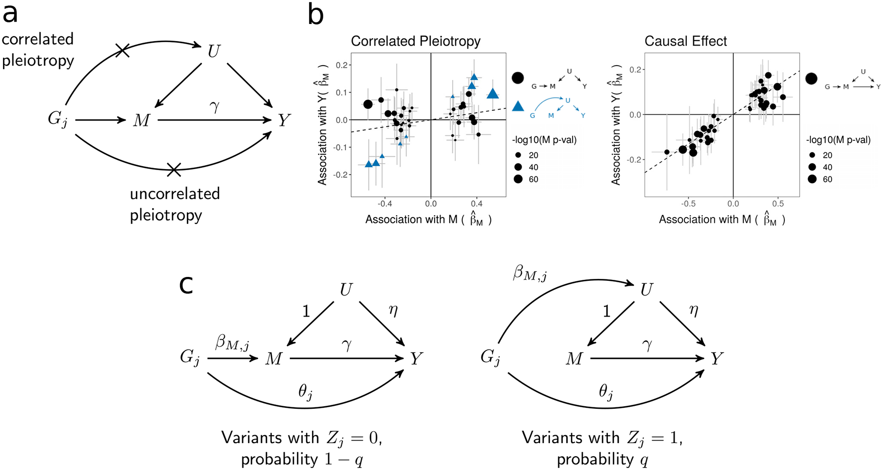
a, Causal diagram assumed by traditional MR approaches. The causal effect of trait M on trait Y, γ, is the target of inference. Crosses mark horizontal pleiotropic effects that are assumed absent by traditional MR. b, Simulated effect estimates illustrating the pattern induced by a shared factor (correlated pleiotropy) with no causal effect (left), and the pattern induced by a causal effect (right). In both plots, effect size estimates for M and Y are indicated by points. Error bars around points have length 1.96 times the simulated standard error of the estimate on each side. SE’s are simulated with a sample size of 5,000. Only variants that are strongly associated with M (p < 5 · 10−8) are shown. c, CAUSE assumes that variants affect trait M through one of two mechanisms. A proportion 1 − q of variants have the left causal diagram, while the remaining proportion, q, have the right causal diagram.
A variant that affects both M and Y through a pathway not mediated by a causal effect is termed horizontally pleiotropic. Horizontal pleiotropy leads to false positives in methods that assume the relationship in Equation (1) and is unfortunately common6,7. Accounting for horizontal pleiotropy has therefore been a major focus of ongoing MR research4. It is helpful to distinguish between two types of horizontal pleiotropy: uncorrelated pleiotropy, where horizontal effects on Y are uncorrelated with effects on M, and correlated pleiotropy, where horizontal effects on Y are correlated with effects on M. Uncorrelated pleiotropy occurs when a variant affects Y and M through separate mechanisms, whereas correlated pleiotropy occurs when a variant affects Y and M through a shared heritable factor, U, such as a shared process or pathway (Fig. 1a). Both types of pleiotropy may occur for any pair of traits.
Of the two types, uncorrelated pleiotropy is easier to account for. If it is mean zero, it only adds noise to the relationship in Equation (1). Multiple methods have been proposed to deal with this, including Egger regression8,9, which allows for directional (non-mean zero) uncorrelated pleiotropy, and methods that rely on outlier removal, including GSMR10 and MR-PRESSO7. Correlated pleiotropy results in correlation between βM,j and βY,j for a subset of variants. This leads to false positives if it is not accounted for. Genetic correlation has been found between many pairs of traits including some that are unlikely to be causally linked, suggesting that correlated pleiotropy is common and may be an important source of MR false positives11–14.
If a suspected shared factor is measured, false positives can be avoided by eliminating variants associated with the shared factor or adjusting for it using multivariable MR15. Two methods, the weighted median16 and the weighted mode17, allow for some correlated pleiotropy. In their unweighted versions, the median and mode estimators assume that fewer than half of variants display horizontal pleiotropy and that the modal horizontal pleiotropic effect is zero, respectively. Another method, LCV14, does not directly test for a causal effect, but estimates the “genetic causality proportion”, with higher magnitude estimates suggesting a causal effect and lower magnitude estimates suggesting correlated pleiotropy.
We present a new MR method that accounts for both uncorrelated and correlated pleiotropy, Causal Analysis Using Summary Effect Estimates (CAUSE), using genome-wide summary statistics. The intuition behind CAUSE is that a causal effect of M on Y leads to correlation between βM,j and βY,j for all variants with non-zero effect on M, while a shared factor induces correlation for only a subset of M effect variants (Fig. 1b). CAUSE uses this distinction to differentiate causal effects from correlated pleiotropy. Unlike many existing methods, CAUSE incorporates information from all variants, rather than only those most strongly associated with M. This can improve power when the GWAS for trait M is underpowered. CAUSE provides a test-statistic, an estimate of the causal effect, and a variant-level summary indicating how each variant contributes to the overall test, and which variants are likely to be acting through a shared factor.
We demonstrate in simulations that CAUSE makes fewer false detections in the presence of correlated pleiotropy than existing methods. In applications to GWAS data, CAUSE identifies plausible causal relationships while avoiding many likely false positives. CAUSE fills a gap in existing methodology by accounting for correlated pleiotropy created by unknown or unmeasured shared factors.
Results
CAUSE models uncorrelated and correlated pleiotropy
CAUSE assesses whether genome-wide effect estimates for M and Y are consistent with a causal effect. In a simple MR analysis, variants with strong associations with M are selected and assumed to follow the causal diagram in Figure 1a. In our proposal, illustrated in Figure 1c, we use all variants but assume that most have no effect on either trait. We assume that the majority of variants that do affect M follow the left-hand causal diagram in Figure 1c, which is the same as the diagram in Figure 1a with the addition of an uncorrelated pleiotropic effect. We allow a small proportion, q, of M effect variants to follow the right-hand causal diagram in Figure 1c, acting on M and Y through an unobserved heritable shared factor, U. Under this model, the relationship between βY,j andβM,j is:
| #(2) |
where Zj is an indicator that is 1 if Gj acts on M through U and 0 otherwise, and η is the effect of U on Y. This relationship is an extension of Equation (1) that includes terms allowing for both types of horizontal pleiotropic effects. We assume that q is small, so Zj is equal to 0 for most variants (see Methods).
Equation (2) captures the patterns in Figure 1b. If γ = 0 and q = 0 (no causal effect and no shared factor), then βY,j and βM,j are uncorrelated for all j. If there is a shared factor and no causal effect (γ = 0, q and η non-zero), then βY,j and βM,j are correlated for variants with Zj = 1 (Fig. 1b, left). If there is a causal effect (γ ≠ 0), βY,j and βM,j are correlated for all variants (Fig. 1b, right). Including all variants allows us to model uncertainty about variant effects on M and gain information from weakly associated variants (see Methods). For computational simplicity, we use a likelihood for independent variants and prune variants for LD before estimating posterior distributions and computing test statistics (see Methods and Supplementary Note, Section SN4).
We assess whether GWAS summary statistics for the two traits are consistent with a causal effect by comparing two nested models. The sharing model has γ fixed at 0, allowing for horizontal pleiotropic effects but no causal effect, and the causal model in which γ is a free parameter. We compare the models using the expected log pointwise posterior density18 (ELPD), a Bayesian model comparison approach that estimates how well the posterior distributions of a particular model are expected to predict a new set data (see Methods). We produce a one-sided p-value testing that the sharing model fits the data at least as well as the causal model. If this hypothesis is rejected, we conclude that the data are consistent with a causal effect.
The right-hand causal diagram in Figure 1c is related to the model used in the latent causal variable (LCV) method14 (see Supplementary Note, Section SN5). Unlike other MR methods, LCV does not provide a test for a causal effect. LCV considers the proportion of heritability of each trait that is mediated by a shared factor, summarized as the “genetic causality proportion” (GCP), which ranges from −1 to 1. A causal model has a GCP of 1 or −1, depending on the direction of effect. O’Connor and Price14 consider a large magnitude estimated GCP more likely to be causal and use a threshold of 0.6 to identify suggestive pairs.
CAUSE can distinguish causality from correlated pleiotropy in simulations
We simulate summary statistics with realistic LD patterns to assess CAUSE in a variety of scenarios and compare performance with other MR methods. Both traits are simulated with a polygenic trait architecture—an average of 1,000 variants with normally distributed effects contribute to a total heritability of 0.25. The power of trait M and Y GWAS can influence performance of all methods, so we consider low power and high power (median 8 and 107 genome-wide significant loci) settings for both traits. Power is controlled by adjusting the simulated GWAS sample size and genome-wide significance is defined as p < 5 · 10−8. We generate effects on trait Y from the relationship in Equation (2) and then simulate effect estimates from true effects and LD structure using results of Zhu and Stephens19 (see Methods).
We compare CAUSE to six MR methods: IVW regression using multiplicative random effects20, Egger regression with random effects8, GSMR10, MR-PRESSO7, the weighted median16, and the weighted mode17. IVW regression, Egger regression, GSMR and MR-PRESSO assume that no variants exhibit correlated pleiotropy. The weighted median and weighted mode methods each allow some horizontal pleiotropy of any kind. All six alternative methods require selection of variants with strong evidence of association with trait M. We follow common practice selecting variants with p < 5 · 10−8 for association with M and pruning for LD so that no pair of variants has pairwise r2 > 0.1.
We first evaluate the robustness of each method to correlated pleiotropy by simulating data with no causal effect and a proportion q = 0 to 0.5 of variants acting through a shared factor, considering weak and strong shared factor effects (Fig. 2a). CAUSE controls the false positive rate in the presence of correlated pleiotropy (q > 0) better than other methods except for Egger regression and the weighted mode. CAUSE makes more false detections when q is large, the confounder effect is large, and both GWAS have high power. This is expected because the data pattern resulting from a high proportion of shared variants is similar to the pattern that results from a causal effect. Although in these settings CAUSE has a higher false positive rate when the trait M GWAS has higher power, as sample size and GWAS power continue to increase, CAUSE’s false positive rate eventually drops to zero, indicating that, asymptotically, CAUSE is able to determine the correct model (Supplementary Note, Section SN6.4).
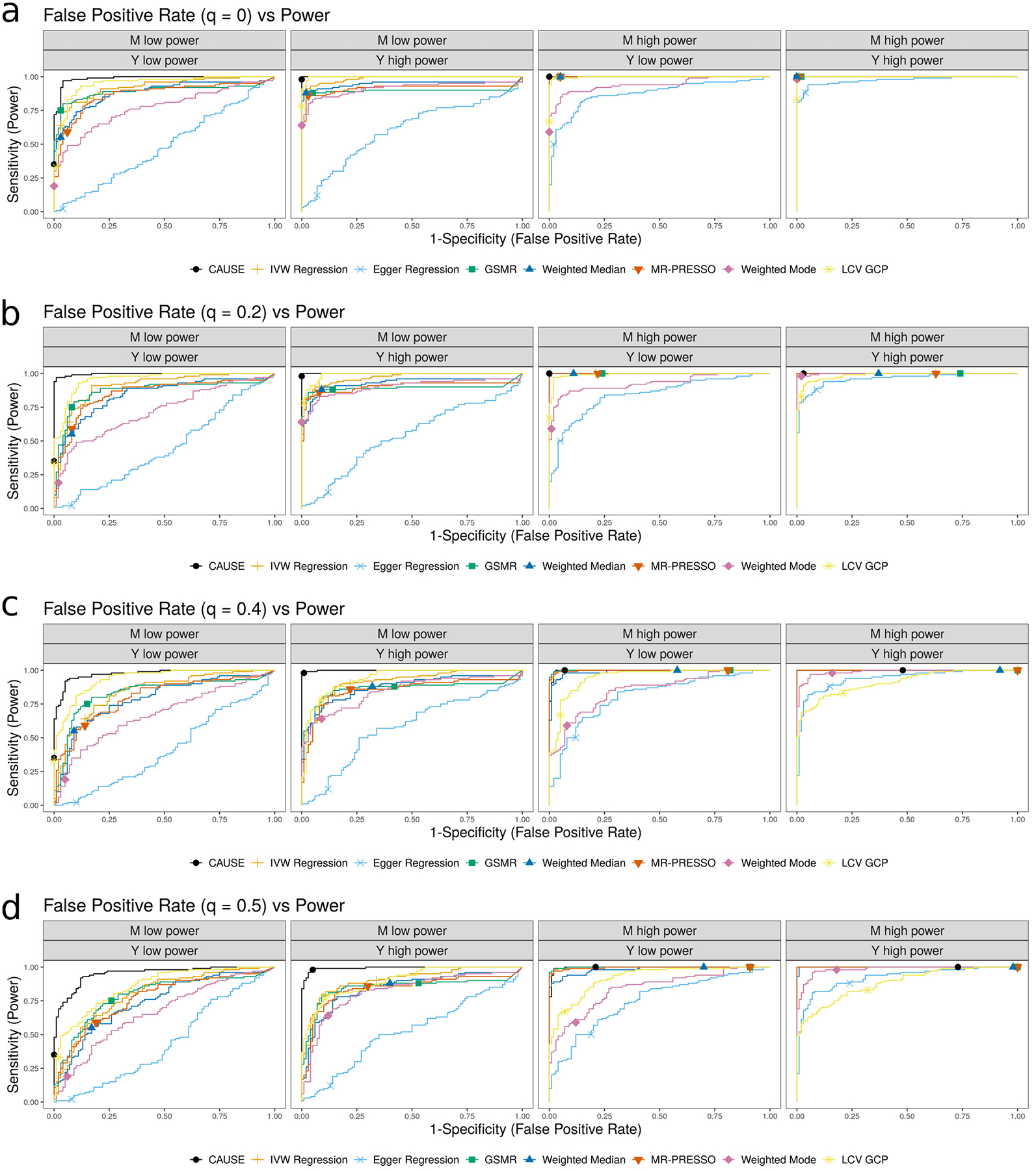
Figure 2 |. Performance of CAUSE and other MR methods in simulated data.
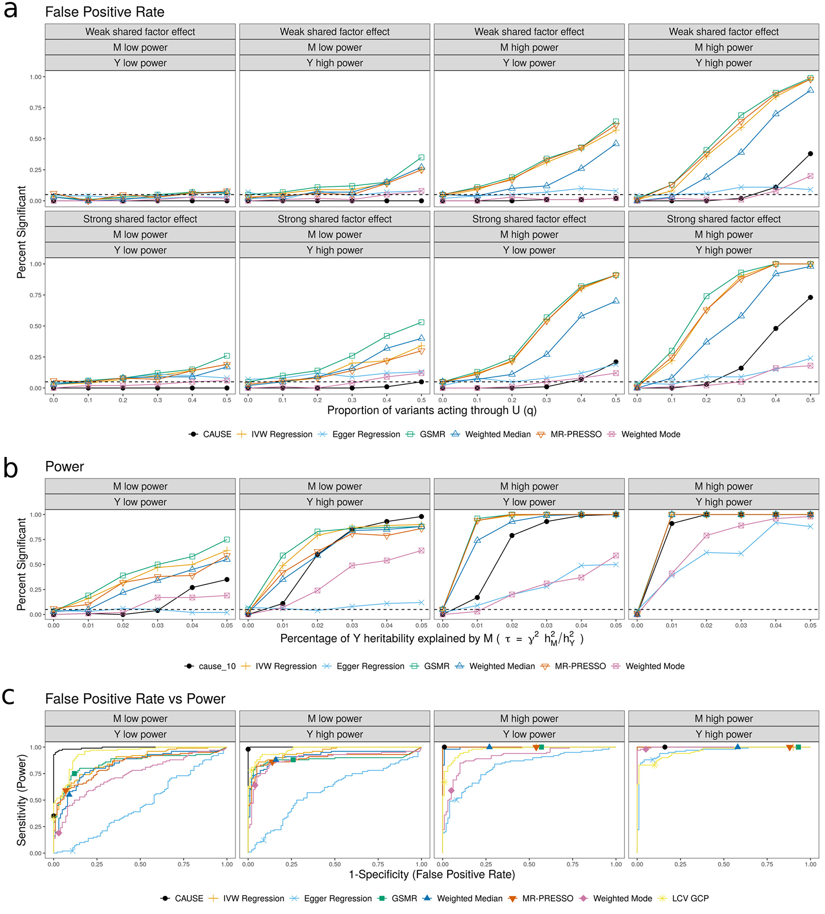
a, False positive rate averaged over 100 simulated data sets in settings with no causal effect and a proportion of correlated pleiotropic variants ranging from 0 to 50%. b, Power averaged over 100 simulated data sets in settings with a causal effect and no shared factor. c, Comparison of false positive-power trade-off. We compare the power when and q = 0 to the false positive rate γ = 0, q = 0.3 and . There are 100 simulations each in the causal and non-causal scenarios. Curves are created by varying the significance threshold. Points indicate the power and false positive rate achieved at a threshold of p ≤ 0.05 or for LCV.
We next compare the power of each method when there is a true causal effect of M on Y and no shared factor (Fig. 2b). CAUSE has substantially better power than Egger regression and the modal estimator, the two methods that control the false positive rate for high levels of correlated pleiotropy. CAUSE has somewhat lower power than other methods in most settings. However, when the trait M GWAS has low power and the trait Y GWAS has high power, CAUSE can achieve better power than other methods for larger causal effects. This is a result of using all variants, rather than only those reaching genome-wide significance. The posterior median of γ can be taken as a point estimate of the causal effect. This estimate tends to be shrunk slightly towards zero compared to alternative methods but has a substantially lower mean squared error than estimates obtained using the weighted mode or Egger regression (Supplementary Note, Section SN6.2). In simulations with both a causal effect and a shared factor, CAUSE maintains similar power when η has a smaller magnitude than γ but loses power when η is large and has opposite sign to γ (Supplementary Note, Section SN6.3).
Although in many settings CAUSE has both lower power and lower false positive rate than other methods, the difference between CAUSE and other methods is not simply calibration. In Figure 2c, we compare the trade-off between power and false positive rate for CAUSE and other methods, additionally including the LCV GCP estimate. CAUSE is better able to distinguish a causal scenario from a non-causal scenario with 30% correlated pleiotropy. This pattern is consistent for levels of correlated pleiotropy between 0% and 50% (Extended Data Fig. 1 and Supplementary Table 1). Additionally, CAUSE is better or equal to other methods at discriminating scenarios with a causal effect and a shared factor from those with only a shared factor (Supplementary Note, Section SN6.3).
CAUSE reduces false positives due to reverse causality
Many MR methods obtain false positives when there is a causal effect of Y on M, but a test is performed for an effect of M on Y (reverse causal effects). This occurs because if Y affects M, some variants will have correlated effects on both traits. However, for most polygenic traits, there will be some variants that affect M through pathways independent of Y and therefore do not exhibit this correlation. By modeling a subset of correlated pleiotropic variants, CAUSE can avoid false positives due to reverse causality as long as only a proportion of M effect variants act through Y.
To verify this expectation, we simulate data with a causal effect of Y on M and no shared factor and test for an effect of M on Y using CAUSE and other methods. In all scenarios, the expected heritability of both M and Y is 0.25. For trait Y, 1000 variants with normally distributed effects explain this heritability. The causal effect of Y on M explains 20% of the trait M heritability while the rest comes from a set of 250, 500, or 1,000 variants (see Methods). CAUSE and the modal estimator both avoid false positives in all settings while the other methods do not (Fig. 3). More false positives from other methods occur when a higher proportion of M effect variants act through Y and therefore have correlated effects. Some false positives from alternative methods could be avoided by carefully filtering variants, for example using Steiger filtering21.
Figure 3 |. False positives resulting from reverse causal effects.
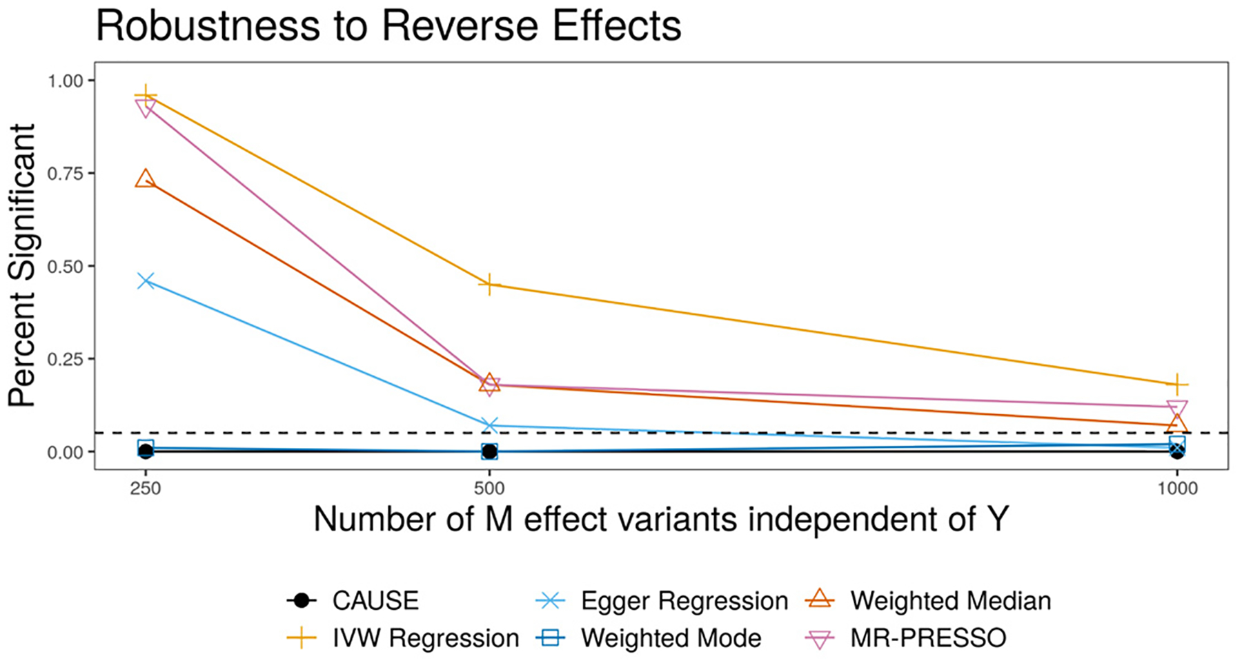
Data are simulated with a true effect of Y on M, but tests are performed for an effect of M on Y. Each point shows the average over 100 simulations. Only CAUSE and the weighted mode control the false positive rate.
Although CAUSE is often able to avoid false positives from reverse causality, it may still find evidence of causality in both directions for some pairs of traits. This can occur for several reasons. First, there may be a causal effect in one direction that accounts for nearly all of the heritability of the downstream/child trait. Second, there may be causal effects in both directions. Third, the two traits may be very closely related and share nearly all genetic variants despite having no causal relationship.
Identifying causal risk factors of common diseases
We use CAUSE and other methods to test for causal effects of twelve possible risk factors for cardio-metabolic diseases on coronary artery disease (CAD), stroke, and type 2 diabetes (T2D) (Supplementary Table 2). In order to increase the number of tested relationships that are unlikely to be causal, we also test for effects of each risk factor on asthma, though not all of these relationships are negative controls. Focusing on well-studied risk factors and diseases allows us to compare results of each method with evidence from scientific literature.
Table 1 summarizes p-values and estimated effect direction for each method as well as GCP estimates from LCV and genetic correlation estimates from LD-score regression (complete results in Extended Data Fig. 2 and Supplementary Table 3). Full lists of variants used for each MR method are provided in Supplementary Table 4. We classified trait pairs in Table 1 by evidence of causality from existing literature (see Supplementary Note, Section SN7) and ordered them by genetic correlation p-value. CAUSE obtains a p-value less than 0.05 for 8 of 9 relationships in the considered causal category, and for 4 of 10 relationships with literature support. Of the remaining pairs in these two categories, 4 are not identified as causal by any method. The remaining negative results from CAUSE are discussed in Supplementary Note, Section SN8. Using LCV, very few pairs of traits have estimated GCP larger than 60%, the threshold used by O’Connor and Price14 as suggestive of a causal relationship. Variant estimates for smoking and CAD, a strong causal effect detected by all methods except LCV, are shown in Figure 4a colored by individual variant contribution to the CAUSE test statistic. Although there is some heterogeneity in effect size correlation, the large number of variants with correlated effects provide enough evidence for CAUSE to reject the sharing model in favor of the causal model.
Table 1 |. Summary of results for pairs of GWAS traits categorized by prior information about causality.
Columns 2–7 give the p-value for each MR method. Values are bold if p < 0.05. Arrows indicate the sign of the corresponding effect estimate. LCV GCP and LCV pval give estimated GCP from LCV and p-value testing that GCP = 0. Values are bold if estimated GCP > 0.6. The Cause q column gives the posterior median of q in the CAUSE sharing model. GC and GC pval give the genetic correlation and p-value testing that genetic correlation is zero estimated by LD score regression. In each section, pairs are ordered by increasing genetic correlation p-value. BF, body fat; BMI, body mass index; BW, body weight; CAD, coronary artery disease; DBP, diastolic blood pressure; FG, fasting glucose; HDL, high-density lipoprotein; LDL, low-density lipoprotein; SBP, systolic blood pressure; TG, triglycerides; T2D, type 2 diabetes.
| Traits | CAUSE | IVW | Egger | Wtd Med | Wtd Mode | MR-PRESSO | LCV GCP | LCV pval | CAUSE q | GC | GC pval |
|---|---|---|---|---|---|---|---|---|---|---|---|
| Considered causal | |||||||||||
| SBP → CAD | 6.6 · 10−31 ↑ | 1.8 · 10−148 ↑ | 7 · 10−18 ↑ | 1.8 · 10−157 ↑ | 3.8 · 10−8 ↑ | 1.3 · 10−167↑ | 0.02 | 0.95 | 0.91 | 0.35 | 2.1 · 10−49 |
| DBP → CAD | 1.3 · 10−26 ↑ | 8.1 · 10−111 ↑ | 5.9 · 10−21 ↑ | 6.4 · 10−138 ↑ | 1.6 · 10−7 ↑ | 1.7 · 10−132 ↑ | 0.54 | 0.069 | 0.88 | 0.27 | 1.3 · 10−27 |
| Smoking → CAD | 9.2 · 10−8 ↑ | 5.4 · 10−11 ↑ | 0.014 ↑ | 1.7 · 10−15 ↑ | 0.00034 ↑ | 1.6 · 10−11 ↑ | 0.44 | 0.21 | 0.65 | 0.22 | 2.3 · 10−27 |
| SBP → Stroke | 4.1 · 10−9 ↑ | 9.3 · 10−93 ↑ | 9.2 · 10−25 ↑ | 5.1 · 10−56 ↑ | 2.2 · 10−7 ↑ | 3.4 · 10−82 ↑ | 0.14 | 0.16 | 0.77 | 0.33 | 1.8 · 10−19 |
| DBP → Stroke | 0.0011 ↑ | 1.2 · 10−77 ↑ | 1.1 · 10−17 ↑ | 1.1 · 10−54 ↑ | 2.6 · 10−7 ↑ | 1.2 · 10−73 ↑ | 0.17 | 0.054 | 0.64 | 0.28 | 1.9 · 10−11 |
| Smoking → Stroke | 0.023 ↑ | 0.00068 ↑ | 0.0062 ↑ | 0.026 ↑ | 0.21 ↑ | 0.00073 ↑ | 0.47 | 0.28 | 0.27 | 0.22 | 5.8 · 10−11 |
| LDL → CAD | 6.3 · 10−12 ↑ | 1.9 · 10−79 ↑ | 5.6 · 10−19 ↑ | 1.5 · 10−50 ↑ | 4.2 · 10−51 ↑ | 2.7 · 10−52 ↑ | 0.87 | 3.6 · 10−57 | 0.79 | 0.19 | 2.9 · 10−5 |
| Smoking → T2D | 0.67 ↑ | 0.11 ↑ | 0.23 ↓ | 1 ↓ | 0.86 ↑ | 0.077 ↑ | 0.05 | 0.69 | 0.05 | 0.04 | 0.19 |
| LDL → Stroke | 0.046 ↑ | 1.2 · 10−5 ↑ | 0.00032 ↑ | 0.0097 ↑ | 0.002 ↑ | 5.2 · 10−6 ↑ | 0.39 | 0.62 | 0.09 | 0.03 | 0.5 |
| Supported by literature | |||||||||||
| BMI → CAD | 0.00012 ↑ | 6.9 · 10−15 ↑ | 0.12 ↑ | 3.5 · 10−17 ↑ | 4.9 · 10−12 ↑ | 8.7 · 10−18 ↑ | 0.49 | 1.2 · 10−9 | 0.56 | 0.23 | 3.1 · 10−24 |
| TG → CAD | 0.085 ↑ | 4.7 · 10−15 ↑ | 0.0023 ↑ | 2.4 · 10−18 ↑ | 6.4 · 10−8 ↑ | 7.3 · 10−18 ↑ | 0.94 | 7.8 · 10−70 | 0.59 | 0.28 | 2.6 · 10−20 |
| BMI → T2D | 0.0048 ↑ | 9.1 · 10−14 ↑ | 0.0089 ↑ | 2.5 · 10−12 ↑ | 3.9 · 10−9 ↑ | 3.9 · 10−14 ↑ | 0.49 | 0.002 | 0.54 | 0.34 | 4.3 · 10−15 |
| BF → CAD | 0.33 ↑ | 0.52 ↑ | 0.93 ↓ | 9.8 · 10−5 ↑ | 8.6 · 10−5 ↑ | 0.78 ↑ | 0.09 | 0.053 | 0.05 | 0.26 | 5.2 · 10−12 |
| BF → T2D | 1 ↑ | 0.046 ↑ | 0.026 ↑ | 1.1 · 10−8 ↑ | 1.1 · 10−7 ↑ | 0.019 ↑ | −0.46 | 0.0073 | 0.04 | 0.38 | 4.3 · 10−9 |
| FG → T2D | 0.013 ↑ | 0.01 ↑ | 0.29 ↓ | 0.0011 ↑ | 0.62 ↑ | 1 · 10−4 ↑ | 0.07 | 0.85 | 0.29 | 0.62 | 7.8 · 10−9 |
| Height → CAD | 0.00018 ↓ | 2.4 · 10−14 ↓ | 0.14 ↓ | 2.8 · 10−12 ↓ | 0.00052 ↓ | 2 · 10−17 ↓ | 0.07 | 0.53 | 0.44 | −0.1 | 1.1 · 10−7 |
| BMI → Stroke | 0.23 ↑ | 0.12 ↑ | 0.73 ↓ | 0.59 ↑ | 0.81 ↑ | 0.1 ↑ | 0.48 | 0.19 | 0.07 | 0.13 | 1 · 10−4 |
| BF → Stroke | 1 ↑ | 0.88 ↓ | 0.7 ↓ | 0.93 ↓ | 0.94 ↑ | 0.83 ↓ | −0.18 | 0.8 | 0.04 | 0.2 | 7 · 10−4 |
| Smoking → Asthma | 0.5 ↑ | 0.089 ↑ | 0.49 ↑ | 0.12 ↑ | 0.94 ↑ | 0.053 ↑ | 0.06 | 0.5 | 0.04 | 0.1 | 0.0036 |
| Unknown or conflicting evidence | |||||||||||
| SBP → T2D | 0.01 ↑ | 1.2 · 10−12 ↑ | 0.13 ↑ | 2.5 · 10−7 ↑ | 0.044 ↑ | 4.5 · 10−12 ↑ | −0.55 | 0.038 | 0.34 | 0.25 | 2.8 · 10−15 |
| HDL → T2D | 0.056 ↓ | 0.0071 ↓ | 0.6 ↑ | 1 ↓ | 0.84 ↑ | 0.025 ↓ | 0.69 | 4 · 10−5 | 0.1 | −0.31 | 2.1 · 10−12 |
| DBP → T2D | 0.02 ↑ | 5.4 · 10−6 ↑ | 0.25 ↑ | 0.00011 ↑ | 0.0041 ↑ | 1.2 · 10−5 ↑ | −0.13 | 0.48 | 0.27 | 0.19 | 2.7 · 10−10 |
| TG → T2D | 0.15 ↑ | 0.38 ↑ | 0.52 ↑ | 0.23 ↑ | 0.22 ↑ | 0.32 ↑ | 0.44 | 0.34 | 0.13 | 0.28 | 5.2 · 10−10 |
| BW → CAD | 0.0014 ↓ | 0.0021 ↓ | 0.94 ↑ | 0.0099 ↓ | 0.29 ↓ | 0.00013 ↓ | 0.5 | 0.23 | 0.31 | −0.16 | 2.2 · 10−8 |
| BW → T2D | 0.064 ↓ | 0.00019 ↓ | 0.16 ↓ | 0.00043 ↓ | 0.25 ↓ | 6.8 · 10−5 ↓ | 0.44 | 0.44 | 0.12 | −0.26 | 2.1 · 10−7 |
| TG → Stroke | 0.99 ↑ | 0.84 ↓ | 0.1 ↓ | 0.8 ↑ | 0.95 ↑ | 0.9 ↓ | −0.31 | 0.36 | 0.03 | 0.15 | 3 · 10−4 |
| BMI → Asthma | 0.16 ↑ | 0.018 ↑ | 0.064 ↑ | 0.0091 ↑ | 0.065 ↑ | 0.017 ↑ | 0.28 | 0.21 | 0.1 | 0.09 | 0.0031 |
| FG → CAD | 0.25 ↑ | 0.0011 ↑ | 0.24 ↑ | 2.2 · 10−6 ↑ | 9.9 · 10−7 ↑ | 0.00025 ↑ | 0.48 | 0.18 | 0.04 | 0.12 | 0.0049 |
| FG → Stroke | 0.99 ↑ | 0.42 ↑ | 0.031 ↓ | 0.37 ↓ | 0.41 ↓ | 0.37 ↑ | −0.67 | 0.0093 | 0.04 | 0.22 | 0.0082 |
| BF → Asthma | 0.57 ↑ | 0.4 ↑ | 0.93 ↑ | 0.85 ↑ | 0.53 ↓ | 0.36 ↑ | 0.08 | 0.63 | 0.04 | 0.12 | 0.048 |
| BW → Stroke | 0.088 ↓ | 0.12 ↓ | 0.039 ↑ | 0.11 ↓ | 0.21 ↓ | 0.052 ↓ | −0.02 | 0.97 | 0.15 | −0.08 | 0.11 |
| Alcohol → Stroke | 0.25 ↑ | 0.41 ↑ | 0.39 ↓ | 0.87 ↑ | 0.77 ↓ | 0.37 ↑ | 0.1 | 0.71 | 0.07 | 0.06 | 0.13 |
| Height → Stroke | 0.55 ↓ | 0.034 ↓ | 0.53 ↓ | 0.24 ↓ | 0.91 ↓ | 0.077 ↓ | −0.18 | 0.58 | 0.03 | −0.05 | 0.15 |
| LDL → T2D | 0.32 ↓ | 0.00017 ↓ | 0.00068 ↓ | 0.022 ↓ | 0.0064 ↓ | 5.5 · 10−5 ↓ | 0.57 | 4 · 10–13 | 0.13 | 0.05 | 0.24 |
| Alcohol → T2D | 0.99 ↑ | 0.27 ↑ | 0.15 ↑ | 0.26 ↑ | 0.29 ↑ | 0.29 ↑ | −0.24 | 0.51 | 0.03 | −0.03 | 0.41 |
| Alcohol → CAD | 0.82 ↑ | 0.47 ↑ | 0.54 ↑ | 0.06 ↑ | 0.036 ↑ | 0.12 ↑ | −0.08 | 0.85 | 0.03 | 0 | 0.99 |
| Implausible or unsupported | |||||||||||
| Alcohol → Asthma | 0.81 ↓ | 0.57 ↓ | 0.14 ↓ | 0.57 ↓ | 0.43 ↓ | 0.56 ↓ | −0.08 | 0.43 | 0.03 | −0.08 | 0.031 |
| Height → Asthma | 1 ↓ | 0.27 ↓ | 0.56 ↓ | 0.42 ↓ | 0.11 ↓ | 0.69 ↓ | −0.07 | 0.62 | 0.03 | −0.04 | 0.29 |
| SBP → Asthma | 0.76 ↑ | 0.026 ↑ | 0.85 ↑ | 0.73 ↑ | 0.35 ↓ | 0.035 ↑ | −0.02 | 0.93 | 0.04 | 0.03 | 0.4 |
| DBP → Asthma | 0.59 ↑ | 0.79 ↑ | 0.086 ↓ | 0.2 ↓ | 0.15 ↓ | 0.88 ↓ | −0.17 | 0.5 | 0.04 | 0.03 | 0.43 |
| FG → Asthma | 0.35 ↓ | 0.24 ↓ | 0.39 ↓ | 0.025 ↓ | 0.082 ↓ | 0.091 ↓ | 0.2 | 0.099 | 0.06 | −0.05 | 0.56 |
| TG → Asthma | 0.17 ↓ | 0.03 ↓ | 0.51 ↓ | 0.93 ↓ | 0.34 ↓ | 0.065 ↓ | 0.02 | 0.88 | 0.06 | 0.03 | 0.58 |
| Height → T2D | 0.96 ↑ | 0.68 ↓ | 0.3 ↑ | 1 ↓ | 0.9 ↑ | 0.62 ↓ | 0 | 0.75 | 0.03 | −0.01 | 0.7 |
| LDL → Asthma | 0.87 ↓ | 0.65 ↑ | 0.82 ↓ | 0.25 ↑ | 0.61 ↑ | 0.87 ↑ | 0.15 | 0.87 | 0.03 | −0.01 | 0.75 |
| BW → Asthma | 0.73 ↑ | 0.18 ↑ | 0.85 ↑ | 0.14 ↑ | 0.42 ↑ | 0.082 ↑ | −0.02 | 0.5 | 0.04 | −0.01 | 0.83 |
| HDL → Asthma | 1 ↑ | 0.91 ↑ | 0.99 ↑ | 0.52 ↑ | 0.93 ↑ | 0.74 ↑ | −0.02 | 0.76 | 0.03 | −0.01 | 0.84 |
| Considered non-causal | |||||||||||
| HDL → CAD | 0.00044 ↓ | 4.9 · 10−9 ↓ | 0.55 ↓ | 5.0 · 10−11 ↓ | 5.6 · 10−6 ↓ | 1.3 · 10−13 ↓ | 0.67 | 0.0012 | 0.54 | −0.26 | 4.8 · 10−18 |
| HDL → Stroke | 0.27 ↓ | 0.076 ↓ | 0.48 ↑ | 0.07 ↓ | 0.13 ↓ | 0.096 ↓ | 0.67 | 3.5 · 10−8 | 0.04 | −0.15 | 2.3 · 10−5 |
Figure 4 |. Effect size estimates and variant level contribution to CAUSE test statistics for four trait pairs.
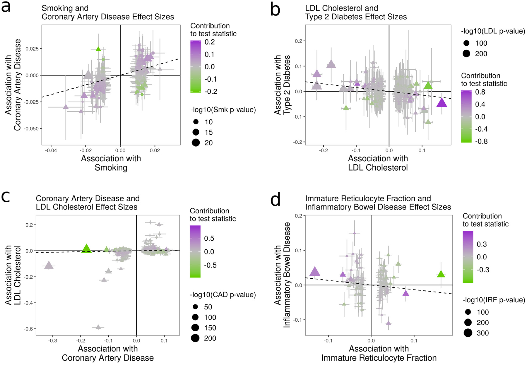
Effect estimates for trait M (horizontal axis) are plotted against estimates for trait Y (vertical axis). Error bars have length 1.96 times the standard error of the estimate. Triangles indicate variants reaching genome-wide significance for trait M (p < 5 · 10−8). Variants with trait M p-value < 5 · 10−6 are shown. Dotted lines show the IVW estimate obtained using only genome-wide significant variants. a, Smoking (M) and CAD (Y). All methods detect evidence of a causal effect. b, LDL (M) and T2D (Y). Only CAUSE does not detect a causal effect. Under the CAUSE model, these data can be explained by a shared factor accounting for 13% of LDL cholesterol effect variants. c, CAD (M) and LDL cholesterol (Y). CAUSE avoids a likely false positive obtained by other methods as a result of a reverse direction effect. Egger regression, the weighted mode, and MR-PRESSO all find a significant effect (see Supplementary Table 5). d, IRF (M) and IBD (Y). MR-PRESSO, the weighted median, and modal estimators obtain a positive result by downweighting or removing variants supplying conflicting evidence.
To assess false positives, we consider traits in the non-causal and implausible categories, and those in the unknown category that have no significant genetic correlation. CAUSE identifies fewer of these pairs as causal than any other method. All methods except Egger regression detect an effect of HDL cholesterol on CAD risk, which is likely to be an error22. This example represents a limitation of CAUSE, as it is possible to obtain false positives when a high proportion of variants are shared. In this case, CAUSE estimates that 54% of variants act through a shared factor.
LDL cholesterol and T2D is an example of a pair of traits identified by other methods but not by CAUSE (Fig. 4b). The true relationship between this pair is unknown. Levels of LDL cholesterol are often elevated in individuals with T2D, an effect that is typically considered a consequence of insulin insensitivity23 (see Supplementary Note, Section SN7). Clinical trials of statins, which reduce LDL cholesterol, show an increased risk of T2D with statin use24,25. However, statins and their target enzyme affect multiple systems, and it remains unknown whether statin effects on T2D are mediated by LDL cholesterol or other mechanisms26 (see Supplementary Note, Section SN7). The effects estimated by IVW regression and other methods are negative, opposite of observational associations, but consistent with previous findings of Fall et al.27. CAUSE does not reject the sharing model (p = 0.32) and estimates that 13% of LDL variants act through a shared factor.
We expect that most effects detected in the opposite direction, of diseases on potential mediators are false positives. Testing opposite direction effects therefore gives us another opportunity to evaluate the robustness of methods to false positives. Additionally, as discussed previously, a reciprocal result for CAUSE can arise from both causal and non-causal scenarios, so it is important to consider tests in both directions. CAUSE identifies five reverse pairs at a p-value threshold of 0.05, fewer than any other method. IVW, Egger regression, the weighted median, the weighted mode, and MR-PRESSO identify 15, 6, 11, 7, and 17 reverse effects respectively (Supplementary Table 5 and Extended Data Fig. 3). The case of CAD and LDL cholesterol provides an example of how CAUSE is able to avoid false positives from reverse effects (Fig. 4c).
All of the mediators in this analysis have high-powered GWAS with many genome-wide significant variants. Such studies are not always available, and simulations suggest that CAUSE may have a power advantage over other methods if the trait M GWAS is underpowered. In order to explore the effect of GWAS power, we compared results using an earlier GWAS for blood pressure with a smaller sample size28. With these data, CAUSE is able to detect effects of blood pressure on CAD that are missed by IVW and Egger regression (Supplementary Note, Section SN9). This suggests that CAUSE may be able to boost power to detect causal effects of mediators with underpowered GWAS.
Links between immune-mediated disease and blood cell counts
There are a growing number of GWAS for intermediate or molecular traits. Relationships between these traits and clinical outcomes are appealing targets for MR studies because molecular traits may be accessible as drug targets or suggest physiological pathways contributing to disease. We use CAUSE and other MR methods to search for evidence of causal relationships between 13 measures of blood cell composition and five immune-mediated diseases (Supplementary Table 6). Results are summarized in Figure 5 and Supplementary Table 7 (full results are shown in Supplementary Tables 8 and 9, and variants used are shown in in Supplementary Table 10).
Figure 5 |. Tests for causal effects of blood cell composition on immune mediated traits.
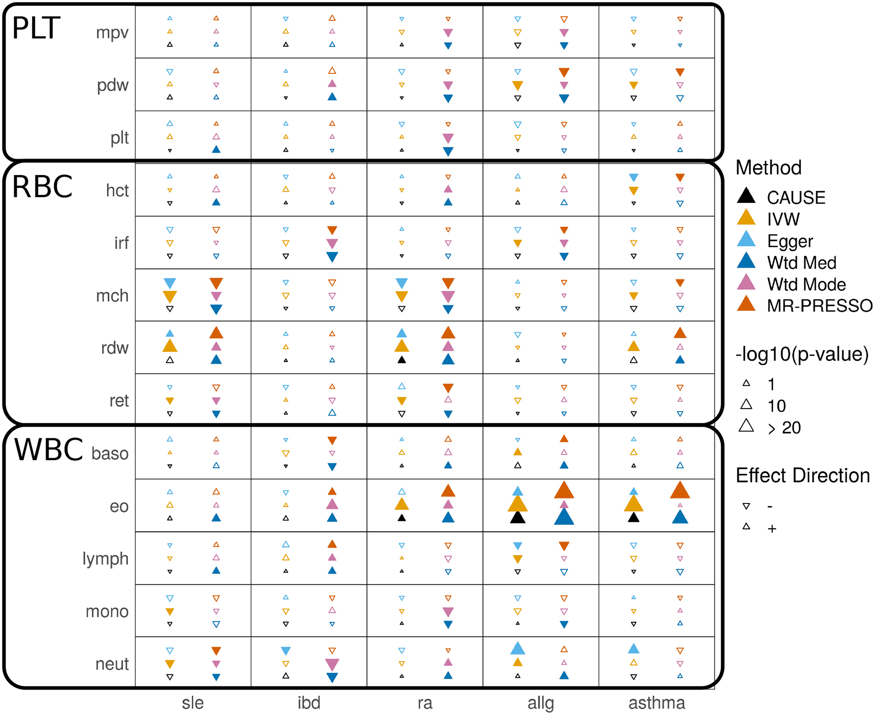
Each cell summarizes the results of six methods for a pair of traits. Filled symbols indicate p-value < 0.05. Blood cell traits are grouped into platelet traits (PLT), red blood cell traits (RBC), and white blood cell traits (WBC).
Blood cell composition traits can be divided into red blood cell, white blood cell, and platelet traits. Although there is less literature information to guide us, we expect that effects of white blood cell traits on immune-mediated disorders are more plausible than effects of red blood cell or platelet traits.
CAUSE identifies only 4 pairs of traits as consistent with a causal effect at p < 0.05. The two most significant effects are positive effects of eosinophil count on asthma and allergy risk (p = 1.9 · 10−5 and 4.0 · 10−11, respectively). Eosinophils have proven to be promising drug targets for treating asthma and allergic disease29. All other methods, including Egger regression and the weighted mode, obtain many more positive results than CAUSE, including likely false positive effects of red blood cell and platelet traits. Some of these results suggest that there are cases when methods that down-weight or remove outliers may be less robust than IVW regression. For example, an effect of immature reticulocyte fraction (IRF, a red blood cell trait) and inflammatory bowel disease (IBD) is found only by the weighted median (p = 1.2 · 10−5), the weighted mode (p = 2.6 · 10−5), and MR-PRESSO (p = 0.0015) (Fig. 4d). There is no visible correlation in variant effect sizes, and CAUSE as well as the simpler IVW regression obtain non-significant results (p =0.32 and 0.16, respectively). By removing or down-weighting the contribution of some variants, putatively robust methods can obtain false positives by discounting conflicting evidence.
Discussion
We have introduced CAUSE, a new approach to MR analysis that accounts for uncorrelated and correlated pleiotropy. Compared to existing methods, CAUSE is able to reduce false positives and, in some circumstances, increase power. Previous authors have identified uncorrelated horizontal pleiotropy as a pervasive phenomenon adversely impacting MR analyses7. Our results demonstrate that correlated horizontal pleiotropy is also common and may explain a substantial fraction of positive MR. Alternative MR methods perform best when information is available to guide removal of pleiotropic variants. For example, in analyzing HDL cholesterol and heart disease, Voight et al.22 avoid a false positive by discarding variants associated with other lipid and metabolic traits. CAUSE does not require such selection and performs well in an automated manner, making it well suited for applications where shared factors are unknown or unmeasured.
Caution must be used when interpreting results of CAUSE, as well as any other MR method. CAUSE tests that the GWAS summary statistics for M and Y are consistent with a model where every M effect variant has a correlated effect on Y. This pattern occurs when M has a causal effect on Y but can also occur in other circumstances. Notably, if most of the heritable variation of two traits is mediated by the same unobserved process, we expect to observe this pattern in both directions. It is therefore good practice to test trait pairs in both directions13. We also note that, while CAUSE is more robust than alternatives, it still has a high false positive rate when a shared factor accounts for a large proportion of the trait M variants. A low p-value from CAUSE (or any MR method) should not be regarded as proof of a causal effect. Instead, it is an indicator that the summary statistics for the two traits are consistent with a causal effect. The power and false positive rate of CAUSE can be affected by the prior on q (Supplementary Note, Section SN6.1). We have chosen a default prior that gives good performance over a range of settings. However, it may also be good practice to conduct sensitivity analyses using more and less stringent priors.
CAUSE has several limitations that provide interesting future directions. First, it is not possible to account for known shared factors when they are measured. Second, CAUSE models only a single unobserved shared factor, so it may not fully account for shared genetic components between two traits of interest. This problem is partially alleviated by the flexibility of the empirical effect size prior distribution (see Methods). Finally, CAUSE prunes variants for LD rather than explicitly modeling variant correlation. This ensures that problem is computationally tractable, but may lead to loss of information.
Methods
CAUSE model for GWAS summary statistics
We use effect estimates and standard errors measured in GWAS of M and Y (summary statistics) to evaluate evidence of a causal effect of M on Y. Let and be effect estimates and standard errors at variant Gj (j = 1, …, p) for traits M and Y, respectively. Let βM,j and βY,j be the true marginal associations of Gj with M and Y. We model effect estimates as normally distributed given the true effects, allowing for global correlation that can result from overlapping GWAS samples. We model:
| #(3) |
where and N2(x; μ, Σ) is the bivariate normal density with mean μ and variance Σ evaluated at x. This model implicitly assumes that and are measured without error. The correlation term, ρ, which accounts for sample overlap, is estimated empirically (Supplementary Note, Section SN1).
In the CAUSE model, a proportion, q, of variants exhibit correlated pleiotropy, modeled as an effect on a shared factor, U (Fig. 1c, right). The remaining proportion, 1 − q, are independent of U (Fig. 1c, left). All variants may have pleiotropic effects, θj on Y that are uncorrelated with their effects on M. Let Zj be an indicator that variant j effects U. Then,
| #(4) |
where η is the effect of U on Y and U is scaled so that the effect of U on M is 1. Note that if there are no uncorrelated or correlated pleiotropic effects, then Equation (4) reduces to βY,j = γβM,j, the relationship assumed by simple MR approaches such as IVW regression. We substitute the right side of Equation (4) into Equation (3) and integrate out Zj to obtain:
| #(5) |
The parameters of interest in the CAUSE model are γ, η, and q. Rather than estimating individual variant effects βM,j and θj, we model their joint distribution empirically and integrate them out to obtain a marginal density for and . We model βM,j and θj as draws from a mixture of bivariate normal distributions. This strategy is based on Adaptive Shrinkage (ASH) approach of Stephens30 for modeling univariate distributions and provides a flexible unimodal distribution with mode at (0,0). We model:
| #(6) |
where Σ0, Σ1, …,ΣK are pre-specified covariance matrices of the form , and π0, π1, …,πK are mixing proportions that sum to 1. The set of parameters Ω = {π0,…,πK, Σ0, …,ΣK} are estimated from the data along with ρ in a single pre-processing step (Supplementary Note, Section SN1). Integrating βM,j and θj out of Equation (5), we obtain:
| #(7) |
where . Treating variants as independent, we obtain a joint density for the entire set of summary statistics as a product over variants. We place independent prior distributions on γ, η, and q, described below, and estimate posterior distributions via adaptive grid approximation (Supplementary Note, Section SN3). A flow-chart illustrating a CAUSE analysis including parameter estimation is shown in Extended Data Figure 4. CAUSE is implemented in an open source R package and we also provide pipelines for running CAUSE on large-scale applications.
Prior distributions for γ, η, and q
We place normal prior distributions with mean zero on γ and η. We find in simulations that results are robust to different choices of prior variance for γ and η, as long the same value is used for both parameters (Supplementary Note, Section SN2). Since the magnitude of a possible causal effect is difficult to know a priori due to differences in trait scaling and covariate adjustment across GWAS, we use the data to suggest a prior variance (Supplementary Note, Section SN2).
By default, and in all analyses presented here, we use a Beta(1,10) prior distribution for q. This distribution gives a prior probability of 0.001 that q > 0.5 and 0.056 that q > 0.25. The parameters of the Beta distribution can be adjusted by the user to reflect different prior beliefs about the size of q. If the prior on q places more weight on values close to zero, CAUSE will behave more similarly to standard MR, obtaining high false positive rates when the true value of q is large. With a more permissive prior on q, CAUSE is more robust to larger amounts of correlated pleiotropy but has reduced power. We set Beta(1,10) as the default choice because it performed acceptably over a range of settings in simulations (Supplementary Note, Section SN6.1).
Accounting for linkage disequilibrium
We treat variants as independent when we compute the joint density of summary statistics. In reality, variants are correlated due to linkage disequilibrium (LD). We define the LD-transformed effects and , where R is the variant correlation matrix and SM and SY are diagonal matrices with diagonal elements (sM,j) and (sY,j)19. We assume that R is the same in both GWAS. The pair of estimates can be approximated as normally distributed with mean and variance S(ρ). If the relationship in Equation (4) holds for true effects, βM,j and βY,j, and either M effects are sparse relative to LD structure (most M effect variants are independent) or q is small, then the relationship between the LD-transformed effects is:
| #(8) |
where (Supplementary Note, Section SN4). In this case, the mean relationship for summary statistics at a single locus is the same with or without LD and Equation (5) and (7) remain valid for variants in LD if βM,j and θj are replaced with and .
Correlations among variants can affect the joint density of all summary statistics, which we compute as a product of the densities at each variant. To account for this, we use a subset of variants with low mutual LD (r2 < 0.1 by default), prioritizing variants with low trait M p-values to improve power.
If M effect variants are dense relative to LD structure and q is large, LD can induce a positive correlation between Y and M effect estimates for all variants, even when there is no causal effect (Supplementary Note, Section SN4). In this case, CAUSE may have an inflated false positive rate.
Model comparison using ELPD
To determine whether GWAS summary statistics are consistent with a causal effect of M on Y we compare a model in which the causal effect is fixed at zero (the sharing model) to a model that allows a non-zero causal effect (the causal model). To compare the fit of these models, we estimate the difference in the expected log pointwise posterior density (ΔELPD)18. The ELPD measures how well the posterior distributions estimated under a given model are expected to predict a hypothetical new set of summary statistics obtained from GWAS of M and Y in different samples.
Let Θ be the set of parameters (γ, η, q). Let pC(Θ|Data) and pS(Θ|Data) be the posterior density of Θ given the observed summary statistics under the causal model and sharing model respectively. Let denote a new observation of . The ELPD for model m ∈ {C, S} (for causal and sharing) is:
| #(9) |
where is given in Equation (7) and ptrue is the probability density under the true data generating mechanism. If ΔELPD = ELPDC − ELPDS is positive, then the posteriors from the causal model predict the data better so the causal model is a better fit. If ΔELPD ≤ 0, then the sharing model fits at least as well, indicating that the data are not consistent with a causal effect.
We estimate ΔELPD and a standard error of the estimator using the Pareto-smoothed importance sampling method described by Vehtari, Gelman, and Gabry18 and implemented in the R package loo. We then compute a z-score, , that is larger when posteriors estimated under the causal model fit the data better than the posteriors estimated under the sharing model. We compute a one-sided p-value by comparing the z-score to a standard normal distribution. The p-value estimates the probability of obtaining a z-score larger than the one observed if the true value of ΔELPD were less than or equal to zero.
Generating simulated summary statistics
To create data with a realistic correlation structure, we estimate LD for 19,490 HapMap variants on chromosome 19 in the CEU 1,000 Genomes population using LDShrink31 (https://github.com/stephenslab/ldshrink) and replicate this pattern 30 times to create a genome sized data set of p = 584,700 variants. We generate effect estimates from the CAUSE model in Equation (4), given setting specific values of γ, η, and q., and parameters defining the trait architecture and power of the GWAS (heritability, number of effect variants, and GWAS sample size).
We simulate an effect estimate and standard error for each variant using the following procedure. First, standardized effects and are drawn from a mixture distribution:
| #(10) |
where fj is the allele frequency of variant j in the 1000 Genomes CEU population. Variances and are chosen to give the desired expected heritability as and . In these simulations, . Parameters πM = mM/p and πθ = mθ/p define the expected number of variants with non-zero values of βM,j and θj respectively. In simulations in Figure 2, mM = mθ = 1,000. Note that is the proportion of trait Y heritability mediated by the causal effect and is the proportion of trait Y heritability mediated by U.
Second, standardized effects are converted to non-standardized effects and standard errors are computed as , where ∙ may be M or Yand NM and NY are GWAS sample sizes for traits M and Y, respectively. Given the other parameters, we selected sample sizes of 40,000 for high powered GWAS settings and 12,000 for low powered GWAS settings to provide desired numbers of genome-wide significant variants (about 107 and 8, respectively).
Third, Zj are drawn from a Bernoulli(q) distribution and true effects βY,j are computed using Equation (4). In Figure 2a, a weak shared factor effects correspond to , while large shared factor effects correspond to . Finally, effect estimates are simulated from true effects as:
| #(11) |
where S. is the diagonal matrix of standard errors and R is the variant correlation matrix19. Simulations can be replicated using the online tutorial (https://jean997.github.io/cause/simulations.html).
Existing MR methods
We compare the performance of CAUSE in simulated data with six other MR methods and LCV14. These are implemented as follows.
Random effect IVW regression, random effect Egger regression, the weighted median, and weighted mode methods are implemented in the MendelianRandomization R package. IVW regression is run using model = “random” and weights = “delta” options. The weighted mode estimator is computed using the phi = 1 and stderror=“delta” options. All other methods are run with default options.
MR-PRESSO is performed using the MRPRESSO R package (https://github.com/rondolab/MR-PRESSO) with outlier and distortion tests.
GSMR is performed using the gsmr R package (http://cnsgenomics.com/software/gsmr/) with the Heidi outlier test, default threshold 0.01, and minimum number of instruments lowered to 1.
LCV is performed using R scripts available from the author (https://github.com/lukejoconnor/LCV) using default parameters.
Reporting summary
Additional details on study design are provided in the Life Sciences Reporting Summary.
Code availability
All software and analysis code is publicly available. The CAUSE method is implemented in an R package available through GitHub.
-
Website: https://jean997.github.io/cause/
Includes pipelines and instructions for replicating all results presented in this paper.
CAUSE software (R package): https://github.com/jean997/cause
Simulations software (R package): https://github.com/jean997/causeSims
Data availability
All of the data analyzed are publicly available with the exception of blood pressure summary statistics from Ehret et al.28. These are available through dbGaP Accession phs000585.v2.p1. Download links for all other data sets are available in Supplementary Table 11. Instructions and code for formatting and processing data and reproducing CAUSE analysis results can be found on the website https://jean997.github.io/cause/.
Extended Data
Extended Data Fig. 1. False positive-power trade-offs for different proportions of correlated pleiotropic variants.
We compare the power when and q = 0 to the false positive rate when γ = 0, q varies from 0 to 0.5 and . There are 100 simulations each in the causal and non-causal scenarios. Curves are created by varying the significance threshold. Points indicate the power and false positive rate achieved at a threshold of p = 0.05.
Extended Data Fig. 2. Tests for casual effects of risk factors on diseases.
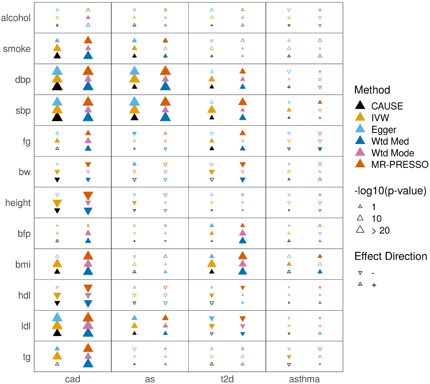
Each cell summarizes the results of six methods for a pair of traits. In the left column of the cell, methods from bottom to top are CAUSE, IVW regression, and Egger regression. In the right column, methods from bottom to top are weighted median, weighted mode, and MR-PRESSO.
Filled symbols indicate a nominally significant p = 0.05.
Extended Data Fig. 3. Tests for casual effects of disease outcomes on risk factors.
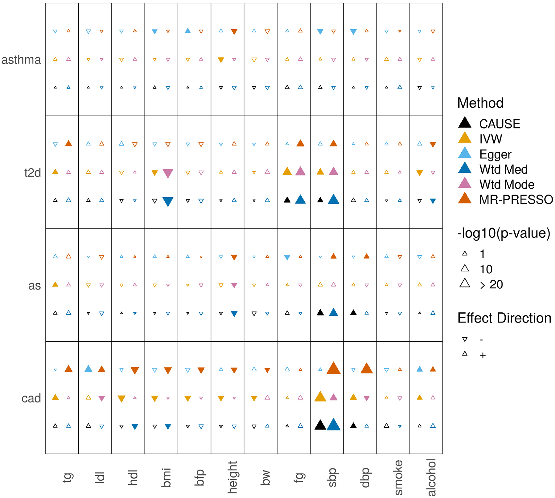
Tests for casual effects of disease outcomes on mediators. Each cell summarizes the results of six methods for a pair of traits. In the left column of the cell, methods from bottom to top are CAUSE, IVW regression, and Egger regression. In the right column, methods from bottom to top are weighted median, weighted mode, and MR-PRESSO.
Filled symbols indicate a nominally significant p = 0.05.
Extended Data Fig. 4. Workflow of a CAUSE analysis.
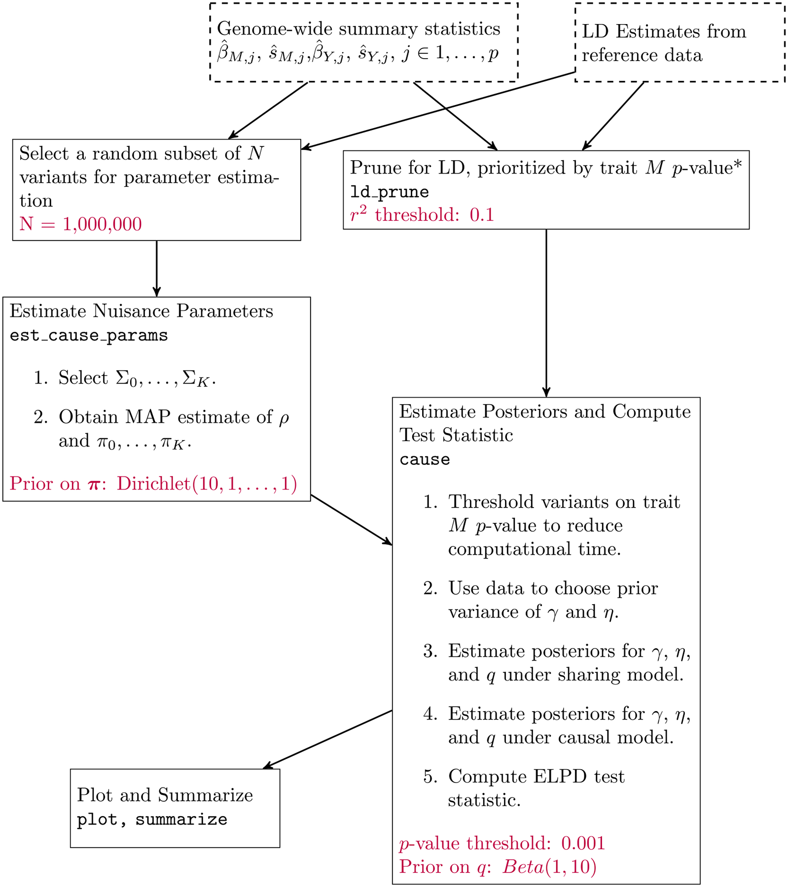
Dashed boxes represent input data. Each solid box is an analysis step completed by the given function in the cause R package. LD pruning can be parallelized over chromosomes. Text at the bottom of boxes indicates user provided parameters and their default values. All analyses presented are run with default parameters.
Supplementary Material
Acknowledgements
This work was supported by National Institutes of Health (NIH) grants MH110531 (to X.H.) and HG002585 (to M.S.), and a Research Grant from the March of Dimes (X.H.).
Footnotes
Competing Interests Statement
The authors declare no competing interests.
References
- 1.Smith GD & Ebrahim S ‘Mendelian randomization’: can genetic epidemiology contribute to understanding environmental determinants of disease? Int. J. Epidemiol 32, 1–22 (2003). [DOI] [PubMed] [Google Scholar]
- 2.Smith GD & Hemani G Mendelian randomization: Genetic anchors for causal inference in epidemiological studies. Hum. Mol. Genet 23, 89–98 (2014). [DOI] [PMC free article] [PubMed] [Google Scholar]
- 3.Boef AGC, Dekkers OM & Le Cessie S Mendelian randomization studies: a review of the approaches used and the quality of reporting. Int. J. Epidemiol 44, 496–511 (2015). [DOI] [PubMed] [Google Scholar]
- 4.Zhang G et al. Genetic associations with gestational duration and spontaneous preterm birth. N. Engl. J. Med 377, 1156–1167 (2017). [DOI] [PMC free article] [PubMed] [Google Scholar]
- 5.Burgess S, Dudbridge F & Thompson SG Combining information on multiple instrumental variables in Mendelian randomization: Comparison of allele score and summarized data methods. Stat. Med 35, 1880–1906 (2016). [DOI] [PMC free article] [PubMed] [Google Scholar]
- 6.Hemani G, Bowden J & Davey Smith G Evaluating the potential role of pleiotropy in Mendelian randomization studies. Hum. Mol. Genet 27, R195–R208 (2018). [DOI] [PMC free article] [PubMed] [Google Scholar]
- 7.Verbanck M, Chen C, Neale B & Do R Detection of widespread horizontal pleiotropy in causal relationships inferred from Mendelian randomization between complex traits and diseases. Nat. Genet 50, 693–698 (2018). [DOI] [PMC free article] [PubMed] [Google Scholar]
- 8.Bowden J, Smith GD & Burgess S Mendelian randomization with invalid instruments: effect estimation and bias detection through Egger regression. Int. J. Epidemiol 44, 512–525 (2015). [DOI] [PMC free article] [PubMed] [Google Scholar]
- 9.Barfield R, Feng H, Gusev A, Wu L & Zheng W Transcriptome-wide association studies accounting for co- localization using Egger regression. Genet. Epidemiol 42, 418–433 (2018). [DOI] [PMC free article] [PubMed] [Google Scholar]
- 10.Zhu Z et al. Causal associations between risk factors and common diseases inferred from GWAS summary data. Nat. Commun 9, 224 (2018). [DOI] [PMC free article] [PubMed] [Google Scholar]
- 11.Bulik-Sullivan B et al. An atlas of genetic correlations across human diseases and traits. Nat. Genet 47, 1236–1241 (2015). [DOI] [PMC free article] [PubMed] [Google Scholar]
- 12.Anttila V et al. Analysis of shared heritability in common disorders of the brain. Science 360, eaap8757 (2018). [DOI] [PMC free article] [PubMed] [Google Scholar]
- 13.Pickrell JK et al. Detection and interpretation of shared genetic influences on 42 human traits. Nat. Genet 48, 709–717 (2016). [DOI] [PMC free article] [PubMed] [Google Scholar]
- 14.O’Connor LJ & Price AL Distinguishing genetic correlation from causation across 52 diseases and complex traits. Nat. Genet 50, 1728–1734 (2018). [DOI] [PMC free article] [PubMed] [Google Scholar]
- 15.Burgess S & Thompson SG Multivariable Mendelian randomization: the use of pleiotropic genetic variants to estimate causal effects. Am. J. Epidemiol 181, 251–260 (2015). [DOI] [PMC free article] [PubMed] [Google Scholar]
- 16.Bowden J, Davey Smith G, Haycock PC & Burgess S Consistent estimation in Mendelian randomization with some invalid instruments using a weighted median estimator. Genet. Epidemiol 40, 304–314 (2016). [DOI] [PMC free article] [PubMed] [Google Scholar]
- 17.Hartwig FP, Smith GD & Bowden J Robust inference in summary data Mendelian randomization via the zero modal pleiotropy assumption. Int. J. Epidemiol 46, 1985–1998 (2017). [DOI] [PMC free article] [PubMed] [Google Scholar]
- 18.Vehtari A, Gelman A & Gabry J Practical Bayesian model evaluation using leave-one-out cross-validation and WAIC. Stat. Comput 27, 1413–1432 (2016). [Google Scholar]
- 19.Zhu X & Stephens M Bayesian large-scale multiple regression with summary statistics from genome-wide association studies. Ann. Appl. Stat 11, 1561–1592 (2017). [DOI] [PMC free article] [PubMed] [Google Scholar]
- 20.Burgess S, Butterworth A & Thompson SG Mendelian randomization analysis with multiple genetic variants using summarized data. Genet. Epidemiol 37, 658–665 (2013). [DOI] [PMC free article] [PubMed] [Google Scholar]
- 21.Hemani G, Tilling K & Davey Smith G Orienting the causal relationship between imprecisely measured traits using GWAS summary data. PLoS Genet. 13, e1007081 (2017). [DOI] [PMC free article] [PubMed] [Google Scholar]
- 22.Voight BF et al. Plasma HDL cholesterol and risk of myocardial infarction: a Mendelian randomisation study. Lancet 380, 572–580 (2012). [DOI] [PMC free article] [PubMed] [Google Scholar]
- 23.Moordian AD Dyslipidemia in type 2 diabetes mellitus. Nat. Clin. Pract 5, 150–159 (2009). [DOI] [PubMed] [Google Scholar]
- 24.Sattar N et al. Statins and risk of incident diabetes: a collaborative meta-analysis of randomised statin trials. Lancet 375, 735–742 (2010). [DOI] [PubMed] [Google Scholar]
- 25.Crandall JP et al. Statin use and risk of developing diabetes: results from the diabetes prevention program. BMJ Open Diabetes Res. Care 5, e000438 (2017). [DOI] [PMC free article] [PubMed] [Google Scholar]
- 26.Swerdlow DI et al. HMG-coenzyme A reductase inhibition, type 2 diabetes, and bodyweight: Evidence from genetic analysis and randomised trials. Lancet 385, 351–361 (2015). [DOI] [PMC free article] [PubMed] [Google Scholar]
- 27.Fall T et al. Using genetic variants to assess the relationship between circulating lipids and type 2 diabetes. Diabetes 64, 2676–2684 (2015). [DOI] [PubMed] [Google Scholar]
- 28.Ehret GB et al. Genetic variants in novel pathways influence blood pressure and cardiovascular disease risk. Nature 478, 103–109 (2011). [DOI] [PMC free article] [PubMed] [Google Scholar]
- 29.Fulkerson PC & Rothenberg ME Targeting eosinophils in allergy, inflammation and beyond. Nat. Rev. Drug Discov 12, 117–129 (2013). [DOI] [PMC free article] [PubMed] [Google Scholar]
- 30.Stephens M False discovery rates: a new deal. Biostatistics 18, 275–295 (2017). [DOI] [PMC free article] [PubMed] [Google Scholar]
- 31.Wen X & Stephens M Using linear predictors to impute allele frequencies from summary or pooled genotype data. Ann. Appl. Stat 4, 1158–1182 (2010). [DOI] [PMC free article] [PubMed] [Google Scholar]
Associated Data
This section collects any data citations, data availability statements, or supplementary materials included in this article.
Supplementary Materials
Data Availability Statement
All of the data analyzed are publicly available with the exception of blood pressure summary statistics from Ehret et al.28. These are available through dbGaP Accession phs000585.v2.p1. Download links for all other data sets are available in Supplementary Table 11. Instructions and code for formatting and processing data and reproducing CAUSE analysis results can be found on the website https://jean997.github.io/cause/.