Absolute quantification of transcription factors reveals principles of gene regulation in erythropoiesis

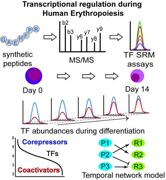
Summary

Dynamic cellular processes such as differentiation are driven by changes in the abundances of transcription factors (TFs). Yet, despite years of studies our knowledge about the protein copy number of TFs in the nucleus is limited. Here, by determining the absolute abundances of 103 TFs and co-factors during the course of human erythropoiesis, we provide a dynamic and quantitative scale for TFs in the nucleus. Furthermore, we establish the first Gene Regulatory Network of cell fate commitment that integrates temporal protein stoichiometry data with mRNA measurements. The model revealed quantitative imbalances in TFs cross-antagonistic relationships that underlie lineage determination. Finally, we made the surprising discovery that in the nucleus, corepressors are dramatically more abundant than coactivators at the protein, but not at the RNA level, with profound implications for understanding transcriptional regulation. These analyses provide a unique quantitative framework to understand transcriptional regulation of cell differentiation in a dynamic context.

Graphical Abstract

eTOC

Protein stoichiometry in the nucleus is mostly unknown. Gillespie et al. use targeted mass spectrometry to quantify over a hundred transcription factors during human erythropoiesis. The data reveal corepressors are on average 100 times more abundant than coactivators. Furthermore, a quantitative model of erythropoiesis integrating mRNA and protein abundances is generated.

Introduction

Quantitative changes in TF abundances drive dynamic cellular processes such as differentiation by activating lineage-specific gene expression programs and simultaneously repressing competing lineages (Graf and Enver, 2009; Orkin and Zon, 2008). At the mechanistic level, biochemical studies have shown that TFs function through the recruitment and/or stabilization of cofactors such as chromatin modifiers to target genes (Brand et al., 2019; Demers et al., 2007). On a more global scale, genomic and transcriptomic studies have uncovered intricate gene regulatory relationships whereby specific combinations of TFs cooperate or compete to regulate cell-specific gene programs (Reiter et al., 2017). The complexity of these relationships is best captured using gene regulatory networks (GRNs) to model the activating and repressing roles of TFs, which underlie lineage fate decisions in multipotent cells such as hematopoietic progenitors (Gottgens, 2015; Novershtern et al., 2011; Rothenberg, 2019; Swiers et al., 2006).

In contrast to the current profusion of transcriptomic data, large-scale quantitative proteomic information is scarce for low abundance proteins such as TFs and cofactors, particularly in human stem/progenitor cells. This critical lack of quantitative proteomic data is a major impediment to addressing fundamental questions in transcriptional regulation, such as TF and cofactor availability in the nucleus (Schmidt et al., 2016). Lack of quantitative proteomic data is also problematic for understanding dynamic processes such a cell fate decisions or differentiation that are based on changes in the stoichiometry of lineage-specifying (LS)-TFs (Graf and Enver, 2009; Orkin and Zon, 2008; Palii et al., 2019). In that regard it is particularly striking that none of the current GRNs for hematopoiesis incorporate quantitative protein abundance data for TFs.

Integration of proteomic data into GRNs is a significant challenge as it requires the ability to measure the abundances of multiple proteins relative to one another (i.e. stoichiometry) within the same sample (Vitrinel et al., 2019), information that cannot easily be obtained with antibody-based methods. Moreover, for dynamic GRNs, the same proteins must be repeatedly measured over time in different samples. While mass spectrometry (MS) is a powerful method for protein identification, absolute quantification is more challenging. A number of approaches have been described for absolute quantification, including the use of synthetic isotopically labeled (SIL) peptides as internal standards, which are typically used for quantification of relatively small numbers of proteins, and label-free methods for large scale quantification [see (Liu et al., 2016) for review]. Both stable isotope dilution (SID) and label-free approaches can be used in conjunction with targeted MS approaches, such as selected reaction monitoring (SRM) which are well-suited for reproducible and quantitative measurements of a defined set of analytes over a wide dynamic range of abundances (Narumi et al., 2016; Simicevic et al., 2013). However, thus far no one has developed and deployed protein detection methods with the required sensitivity and reproducibility to systematically determine the absolute abundances of endogenous TFs and cofactors in rare stem and progenitor cells.

Here, we developed targeted SRM assays in hematopoietic and erythroid nuclear extracts and applied these assays along with SIL peptides as internal standards. This allowed us to systematically determine the absolute abundances of 103 endogenous TFs and co-factors at 13 sequential time points as human hematopoietic stem and progenitor cells (HSPCs) differentiate along the path to erythroid cells. In addition to defining the range of protein concentration (copy number per nucleus) for master regulators of hematopoiesis and erythropoiesis, the data revealed surprising differences in stoichiometry and dynamics between TFs, coactivators and corepressors that occur at the protein level, but not at the RNA level with important implications for understanding gene regulation during differentiation. Finally, through mathematical modeling we generated for the first time a dynamic regulatory network of erythroid commitment from hematopoietic stem cells (HSCs) that integrates quantitative changes in RNA and protein levels (stoichiometry) of TFs over time.

Results

Absolute Quantification of Transcription Factors during Human Erythropoiesis

While proteomic studies have been performed in erythroid cells (Amon et al., 2019; Brand et al., 2004; Gautier et al., 2016 ; Jassinskaja et al., 2017; Liu et al., 2017), no previous study has used targeted MS approaches to provide systematic and absolute quantification of TF proteins with simultaneous mRNA measurements during the dynamic process of erythroid differentiation. Furthermore, previous MS-based studies have not measured TFs in primary human progenitor cells prior to lineage commitment, preventing the study of quantitative changes in TFs that underlie cell fate decisions. To address this, we employed a well-characterized ex vivo culture system in which cord blood-derived human multipotent HSPCs are induced to differentiate along the erythroid lineage (Giarratana et al., 2005; Palii et al., 2011a). Previously, using single cell mass cytometry, we showed that in this system, cells recapitulate all sequential stages of erythropoiesis over time, including multipotent progenitors (MPP) at day 0, common myeloid progenitors (CMP) and megakaryocyte-erythroid progenitors (MEP) at days 2–4, erythroid progenitors “colony-forming-unit erythroid” (CFU-E) at days 6–11, followed by terminally differentiating precursors: pro-erythroblasts (ProEB) at day 12, basophilic erythroblasts (Baso_EB) at day 14 and polychromatophilic erythroblasts (Poly_EB) at day 16 (Palii et al., 2019). Thus, this provides an ideal system for quantitative proteomic and transcriptomic analyses. Cells were harvested at 13 sequential time points and processed in parallel for RNA sequencing (RNAseq) and nuclear protein extraction (Figure S1A). First, RNAseq analysis revealed a main trajectory along two principal components from day 0 to day 16 (Figure S1D). Furthermore, a correlation heatmap indicated that the transcriptome changes gradually throughout the time series with sharper changes at day 2 (transition to CMP/MEP), day 11.5 (transition to ProEB) and day 14 (transition to Baso_EB) (Figures 1E and S2A). For proteomic analyses, nuclear extracts were first analyzed using an unbiased data-dependent MS approach with isobaric 8-plex iTRAQ reagents (Ross et al., 2004) which led to the identification and relative quantification of 3,905 proteins over time (Tables S1 and S2, Figure S1F). Analysis of iTRAQ data allowed identification and relative quantification of 3,905 proteins, including 655 TFs, over time (Table S1). K-means clustering with gene ontology (GO) analyses revealed groups of proteins with enrichment in erythroid-related categories (e.g. “O₂ transport” in Baso_EB (cluster 8), “cell cycle” in the highly proliferative CFU-E populations (cluster 6)) (Figure S1F and Table S2). Furthermore, the GO term “eukaryotic translation initiation” was found enriched in proteins that increase at the ProEB stage (day 12), consistent with the importance of protein translation in terminal erythroid differentiation (Alvarez-Dominguez et al., 2017). Interestingly, we found that proteins involved in oxidative phosphorylation (cluster 3) increase at day 2, which coincides with MPPs commitment to the myeloid/erythroid lineage. Given that oxidative phosphorylation correlates with lineage commitment (Oburoglu et al., 2016), this finding further supports the relevance of our ex vivo differentiation system to reveal molecular events that occur in early hematopoietic progenitors.

Figure 1.

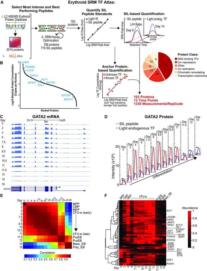
Absolute Quantification of Transcription Factors and Co-factors during Human Erythropoiesis.

(A) Schematic of SRM assay development to quantify TFs and cofactors during hemato/erythropoiesis. Absolute abundance was determined at each time-point using either the SIL-based or the Anchor protein–based quantification method. Two biological replicates were performed. SIL, stable isotope labeled; IS, internal standard.

(B) Range of protein abundances in the nucleus averaged for all time points.

(C) RNA-seq coverage of the GATA2 gene over time as displayed by the UCSC genome browser. Replicate 1 is shown as a representative example.

(D) Quantification of GATA2 protein over time by SRM. Ion chromatograms of endogenous (red) and SIL (blue) EVSPDPSTTGAASPASSSAGGSAAR peptide from the Skyline software. Replicate 1 is shown as a representative example.

(E) Correlation matrix between RNA-seq experiments at the indicated days. The heatmap displays Pearson correlations. Stages of differentiation (indicated on the right) were attributed to the time-points using CyTOF as previously described (Palii et al., 2019).

(F) k-means clustering analysis of normalized protein abundances at the indicated days. Protein abundances were measured by SRM and are shown as a heatmap after normalization.

See also Figures S1, S2, S3, Data S1 and Tables S1, S2, S3, S4.

To systematically determine the absolute concentration of TFs and cofactors, we employed SRM-based targeted MS together with SIL peptide-based quantification (Figure 1A). First, we established an Erythroid SRM TF Atlas consisting of parameters needed to monitor 411 isotopically heavy and light peptide pairs, corresponding to 150 proteins (1–4 peptide pairs per protein) (Tables S3, S4). SRM assay development, including selection of proteotypic peptides, transition ions, and the linear ranges of quantification is described in STAR Methods. Absolute quantification was then achieved by a combination of SID and label free quantification for 103 proteins that span various categories (e.g. DNA binding TFs, co-activators, co-repressors, chromatin modifiers) at 13 sequential time-points from MPP to basophilic erythroblasts (Figure 1A, S2B, Data S1; Table S4; see STAR Methods). Comparing SRM results with iTRAQ measurements, we found a good correlation in protein changes during differentiation (Figure S2C). Importantly, SRM measurements covered a wide dynamic range of nuclear protein abundances, ranging from less than 500 copies for some factors (e.g. BACH1, GATA2, KAT2A) to above 100,000 copies for others (e.g. CTCF, TRIM28/KAP1, CHD4) (Figure 1B). Notably, our CTCF measurements are consistent with copy number estimates obtained using Fluorescence Correlation Spectroscopy in non-hematopoietic cells (Cattoglio et al., 2019). Furthermore, for some proteins, we validated SRM-based quantification with quantitative Western blots (Figure S3).

Using clustering analysis, we identified several groups of temporally-regulated proteins (Figure 1F). Interestingly, all master regulators of erythropoiesis (GATA1, TAL1, KLF1, KLF3, GFI1B, STAT5A) are characterized by a gradual increase from MPP to late CFU-E, followed by a sharp decline starting at the ProEB stage that marks the beginning of terminal erythroid differentiation (Figure 1D, F). This decrease was confirmed by Western blot (Figure S1E). While most factors are present at low levels in terminally differentiated erythroid cells, some TFs are more abundant, including NFE2, MAFG, FOXO3 (Liang et al., 2015), SOX6, STAT1,2 and 3 suggesting additional roles during erythroid maturation. In contrast, TFs that play critical roles in HSC or in promoting non-erythroid lineages (e.g. ETV6, ERG, PU.1, FLI1, RUNX1) are expressed at higher levels at early stages (days 0–4), consistent with lineage priming, and gradually decrease as the cells progressively commit towards the erythroid lineage (Figure 1F). Thus, our differentiation system faithfully mimics the dynamics of erythropoiesis from early to late stages.

Major Discrepancies in Protein versus mRNA Abundances for Master Regulators of Hematopoiesis and Erythropoiesis

Having quantified protein and mRNA abundances simultaneously for multiple TFs (see for example GATA2 in Figure 1C,D), we explored the correlation between mRNA and protein levels. Consistent with previous studies in other cell types (Liu et al., 2016; Vogel and Marcotte, 2012), we found a good protein vs mRNA correlation in cells starting at day 2, with Spearman coefficients ranging from 0.40 to 0.56 (Figure 2A). In contrast, the correlation between mRNAs and proteins is extremely low (<0.25) in early progenitors at day 0 (Figure 2A). This finding, which may be explained by the low protein translation rate in HSCs (Liu et al., 2017; Signer et al., 2014), indicates that post-transcriptional regulation may be particularly important to determine protein abundance in stem/progenitor cells.

Figure 2.

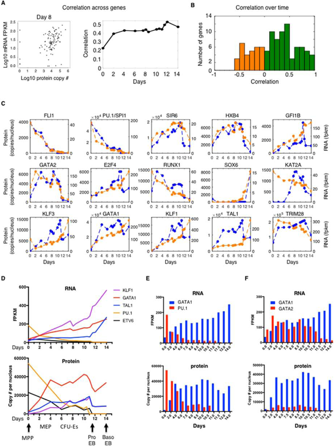
Major Discrepancies in Protein versus mRNA Abundances for Master Regulators of Hemato/Erythropoiesis

(A) Correlation between mRNA and protein abundances at the indicated days. The left panel shows a representative example of a dot plot at day 8 with each dot representing a protein-mRNA pair. The right panel shows the calculated correlation at each day.

(B) Correlation between the changes in mRNA and protein levels over time during differentiation from day 0 to day 14. Positive correlations are in green. Negative correlations are in orange.

(C) Protein (blue) and mRNA (orange) abundances for the indicated genes during differentiation. See Data S2 for all 103 measured genes.

(D) mRNA (top) and protein (bottom) stoichiometry for the indicated genes during differentiation.

(E) mRNA (top) and protein (bottom) stoichiometry for the indicated genes during differentiation.

See also Data S2 and our Human Erythropoiesis TFs website (https://trena.systemsbiology.net/app/srm_rna_combined_v2).

Next, we measured the correlation of mRNA and protein levels over time (Figure 2B). We found that for most genes there is a positive correlation (green bars), indicating that changes in protein levels result in large part from changes in their mRNAs abundance during erythroid differentiation. However, some genes display low or negative correlations (orange bars). Among genes that display a high correlation between mRNA and protein, we found the non-erythroid TFs FLI1 and PU.1 (also called SPI1) both of which decrease gradually during erythropoiesis, but also SOX6, HOXB4 and GATA2 that increase during differentiation (Figure 2C). In contrast, other genes display major discrepancies in protein vs mRNA dynamics (e.g. KAT2A, RUNX1). Interestingly, all master regulators of erythropoiesis (i.e. GATA1, KLF1, KLF3 and TAL1) display a similar pattern of changes with protein levels increasing faster than mRNA levels until the ProEB stage (day 11.5) when they decrease by 40 to 50% even though their transcripts continue to increase (Figure 2C,D). This sharp decline in TF protein levels in the nucleus starting at the ProEB stage was also detected by iTRAQ (Table S1) and Western blot (Figure S1E) and coincides with a drastic change in the transcriptome (Figures 1E and S2A) as the cells enter terminal differentiation. All genes can be explored in Data S2 or on our website (https://trena.systemsbiology.net/app/srm_rna_combined_v2).

An important aspect of transcriptional regulation is the change in relative abundances between TFs. Examining master regulators of hematopoiesis, our results reveal major differences in stoichiometry. For instance, at the transcript level, KLF1 is the most highly expressed TF in erythroid cells (Figure 2D). However, at the protein level, GATA1 is the most abundant TF with over 41,000 copies per nucleus in late CFU-E compared to fewer than 18,000 copies for KLF1, TAL1 or NFE2 (Figure 2D and Table S4). This high abundance of GATA1 protein is likely due to enhanced translation efficiency as shown by polysome profiling (Khajuria et al., 2018; Liu et al., 2017).

In addition to erythroid-specifying TFs, we also quantified TFs that are involved in stem cell maintenance (e.g. ERG, ETV6, RUNX1) and/or specification of alternate hematopoietic lineages (e.g. PU.1, FLI1, CEBPß). Interestingly, even though these non-erythroid factors gradually decrease during differentiation, they are still detectable at the protein and RNA level until late CFU-Es (Figure 2 C,D and Table S4) which suggests some degree of lineage plasticity in late progenitors. In particular, we examined the relative levels of two antagonist TFs GATA1 and PU.1, which promote mutually exclusive hematopoietic lineages (Huang et al., 2007). As expected, we observed a gradual change in the GATA1/PU.1 ratio, at both the RNA and protein levels (Figure 2E) showing that for some factors, RNA levels can be used as a surrogate for protein levels. Another TF switch necessary for erythroid maturation is the GATA switch (Katsumura et al., 2017). It has been shown that during hematopoiesis GATA2 is expressed earlier than GATA1. As erythroid differentiation proceeds, GATA1 progressively represses GATA2 transcription such that when the cells reach the ProEB stage, GATA1 replaces GATA2 on target genes (Huang et al., 2016). It is currently thought that this exchange of GATA2 for GATA1 genomic binding (called the “GATA switch”) is due to GATA2 protein being progressively displaced from its binding sites by increased levels of GATA1 through a competition mechanism. However, even though this view is consistent with our RNA data (Figure 2F top), it is not compatible with our protein measurements. First, we found that GATA1 protein abundance largely exceeds that of GATA2 from the earliest CFU-E stage (Figure 2F bottom) showing that in contrast to the currently accepted model, GATA2 binds to specific genomic sites even in the presence of an excess of GATA1. Furthermore, our data show a decrease (not an increase) in GATA1 protein levels at the proEB transition (Figure 2F bottom - day 10.5 to day 12). Importantly, GATA2 protein levels also decrease (about 10-fold - from 4000 to 400 copies) at this time point. Thus, the most likely explanation for GATA2 decreased genomic binding is not an increase in GATA1 (which does not occur at the protein level at this time point) but a decrease in GATA2, which occurs at the RNA and protein levels (Figure 2C, D, F). The details of the molecular mechanism underlying this switch warrant further investigation.

Notably, we confirmed GATA1 expression in early progenitors by Western blot (Figure S1B), and our finding of a high GATA1/GATA2 protein abundance ratio is consistent with previous data showing both a higher translational efficiency and a higher protein stability of GATA1 compared to GATA2 (Khajuria et al., 2018; Lurie et al., 2008; Minegishi et al., 2005). Thus, while in some cases, transcripts can be used as a surrogate for proteins, in other cases, they cannot, strongly emphasizing the importance of direct protein quantification.

Quantitative Gene Regulatory Model of Erythroid Lineage Commitment

Gene Regulatory Networks (GRNs) provide a useful way to represent complex regulatory relationships that underlie important processes such as cell fate decisions (Dore and Crispino, 2011; Gottgens, 2015; Novershtern et al., 2011; Rothenberg, 2019). However, because of the lack of quantitative proteomic data on TFs, it has not been feasible to build networks that integrate quantitative changes in TF protein levels. Having quantified hematopoietic and erythropoietic TFs at multiple sequential time points, we sought to build a temporal GRN that integrates quantitative changes in protein and mRNA abundances of key TFs (Figure 3). We used both “core” hematopoietic factors with known functions in cell fate decisions (e.g. PU.1, GATA1, GATA2, FLI1, KLF1) and other factors (e.g. ERG, E2F4, KLF3, HOXB4), for a total of 14 genes. Focusing on transcriptional regulation, mathematical modeling with differential equations was used to explain the observed mRNA trajectory of each gene as a function of the observed protein trajectories of candidate regulators. The model is quantitative in that it estimates the relative contribution(s) of distinct TFs to the regulation of their respective targets (represented as transparency of the links – Figure 3B,C,D). Also see Figure 4A,B. Unique to our model, the parameters that quantify regulatory strength are linked to the absolute abundance of proteins. This allows us to discriminate, for example, between a strong activator at low abundance and a weak activator at high abundance (represented as the thickness of the links). First, we found that the model correctly recapitulates the sequential cross-antagonisms between LS-TFs that underlie cell fate decisions, with the GATA1:PU.1 antagonism that regulates erythroid vs myeloid lineage choice (Huang et al., 2007) being detected first (day 0) followed by the KLF1:FLI1 antagonism (day 2) that regulates a subsequent erythroid vs megakaryocyte fate (Frontelo et al., 2007; Palii et al., 2019) (Figure 3B and Movie S1). Strikingly, these cross-antagonisms are not “equilibrated”, with for instance the repression of PU.1 by GATA1 being 3 times stronger than the reverse reaction at day 0, and 19 times stronger at day 4 (Figure 3C). This quantitative imbalance has not been described in previous network models and may reflect an early (but reversible) bias towards the erythroid lineage. Most importantly, our finding that antagonistic relationships between TFs are quantitatively imbalanced provides a mechanism to explain the observed instability of multipotent progenitors that do not exist as stable states but rather as constantly changing entities (Laurenti and Gottgens, 2018). Similarly, our model revealed the dynamics of the FLI1:KLF1 cross-antagonism that starts at day 2, decreases at day 6, and finally disappears at day 8 (Figure 3D). Thus, our proteomic-based network is able to capture the temporal and quantitative aspects of gene regulation to model the dynamics of erythroid lineage commitment. To facilitate visualisation of the network, an interactive version is provided in BioTapestry format (Paquette et al., 2016) at: http://grns.biotapestry.org/HumanErythropoiesisGRN/.

Figure 3.

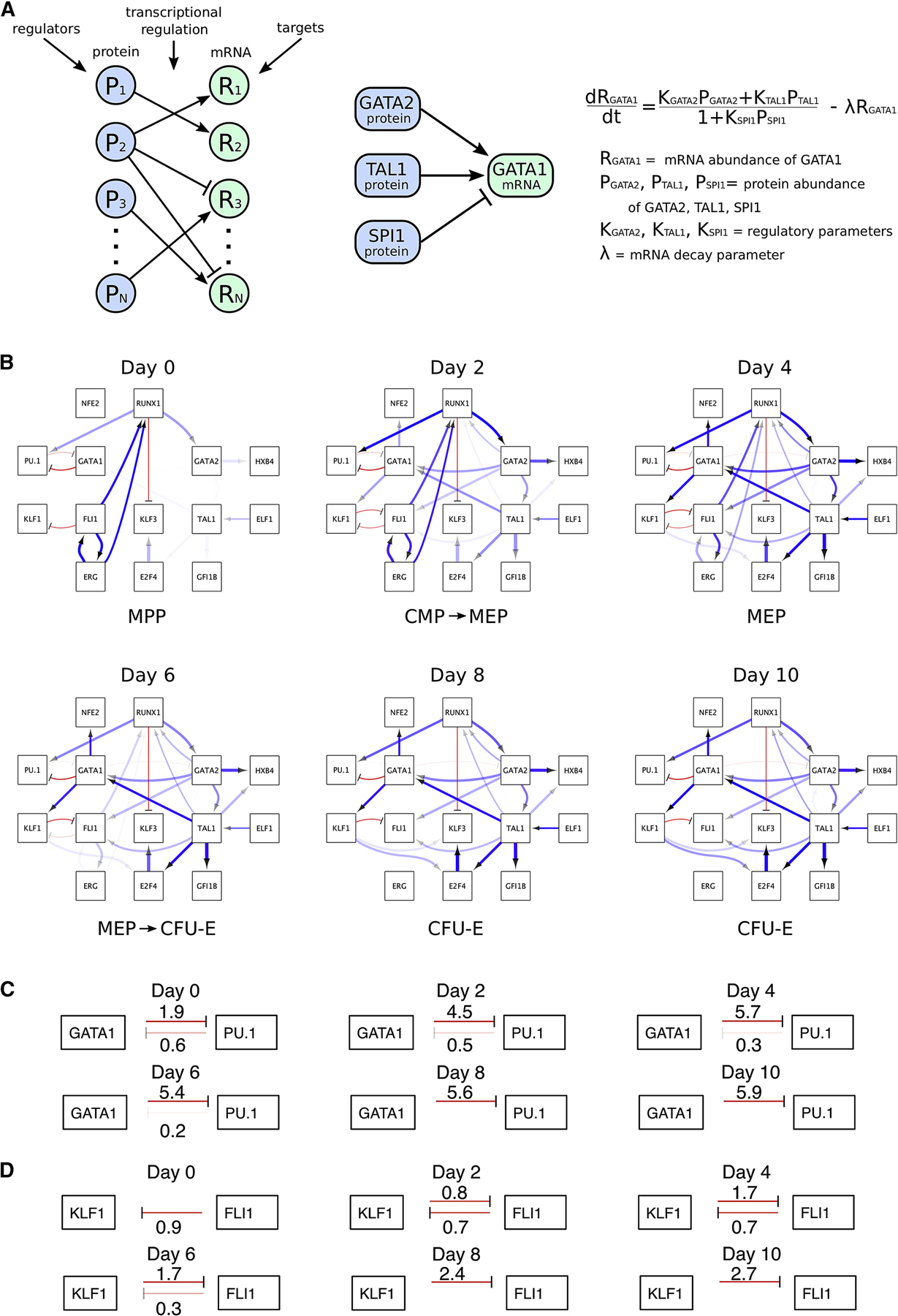
Quantitative Gene Regulatory Network of Erythroid Commitment

(A) Modeling approach: mRNA dynamics are modeled depending on regulator protein abundances. Transcriptional activation is represented as a ratio of two linear functions, corresponding to activation and repression, with constant rates multiplied by protein abundances. mRNA degradation is modelled as a linear decay.

(B) Quantitative Network diagrams depicting dynamic changes in transcriptional regulation of erythroid commitment. Blue and red links indicate activation and repression, respectively. Link transparency indicates the relative contribution of a TF to the regulation of its targets (more transparent links represent weaker effects, depending on regulatory parameter and regulator abundance). Link thickness indicates the regulatory effect per TF protein molecule (thicker links indicate greater regulatory effect per TF protein molecule). The network is also available in BioTapestry format (Paquette et al., 2016) at http://grns.biotapestry.org/HumanErythropoiesisGRN/

(C,D) Quantitative imbalance in the GATA1-PU1 (C) and KLF1-FLI1 (D) cross-antagonistic relationships over time. Excerpt from the network in (B). The strengths of the regulatory relationships are indicated at each time point. Regulatory strength or transparency score was determined from the parameters Ki and Ri as log2(1+Ki*Ri).

See also Table S5 and Movie S1.

Figure 4.

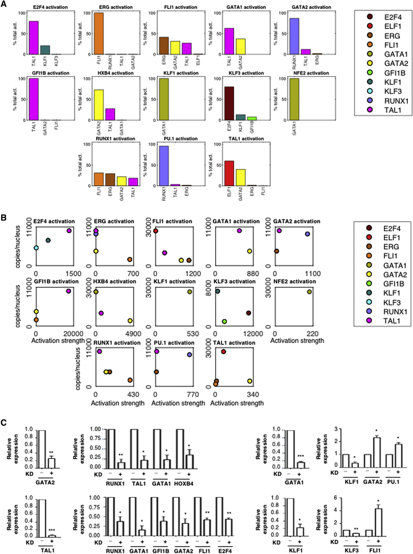
Quantitative Regulatory Relationships

(A) Relative contribution of each TF to the activation of its targets within the GRN. The average activation of a regulator X on target gene Y is computed as A_X*K_XY, where A_X is the average protein expression of gene X over the days 0, 2, 4, 6, 8 and 10, and K_XY is the GRN’s regulatory parameter quantifying its effect on gene Y. The activation percentage is A_X*K_XY divided by the sum of average activations from all activators of Y.

(B) The activation strength of each TF for its target gene is plotted relative to its abundance. For each gene Y in the GRN, the average protein abundance A_X and regulatory parameter K_XY are plotted for all activators X.

(C) The knockdowns of GATA1, GATA2, TAL1 and KLF1 were induced separately by lentiviral delivery of shRNA in cells at day 8. Expression of putative target genes was tested by qRT-PCR after 48h. Expression is shown relative to GAPDH as mean +/− standard error of the mean (SEM). n=3. Two-tailed t-test: * p < 0.05. **p < 0.01. *** p < 0.001.

In addition to TF cross-antagonisms, the model confirmed a number of previously known regulatory links including the GATA1/GATA2 regulatory loop with GATA2 activating GATA1 and GATA1 progressively repressing GATA2 (Katsumura et al., 2017), the ERG-mediated activation of RUNX1 (Taoudi et al., 2011), the TAL1-mediated activation of GATA1 and GFI1B (Gottgens, 2015), the KLF1-mediated activation of KLF3 (Ilsley et al., 2017), the GATA2-mediated activation of HOXB4 (Fujiwara et al., 2012) and others (Figure 3B). Furthermore, the model identified novel putative links such as TAL1- and KLF1-mediated activation of E2F4, E2F4-mediated activation of KLF3, TAL1-mediated activation of HOXB4 and others. These novel regulatory links are likely important for erythropoiesis. For instance, E2F4 has been shown to promote erythropoiesis (Kinross et al., 2006) and our results suggest that this may be mediated at least partially through the activation of KLF3. Most importantly, the model offers a temporal and quantitative view of these regulatory relationships. For instance, we found that over the entire time course, the contribution of TAL1 to the activation of the GATA1 gene is greater than the contribution of GATA2 (with GATA2 being more important at early stages) (Figure 4A). Interestingly, this is not because TAL1 is a stronger activator of GATA1 but instead, this is due to the fact that the TAL1 protein is on average 3 times more abundant than the GATA2 protein (Figure 4B). Thus, the model is able for the first time to quantitatively dissect the relative contributions of different factors to the regulation of their target genes.

To validate our network model, we induced the knockdown of four different TFs (i.e. GATA2, GATA1, TAL1 and KLF1), followed by qRT-PCR assessment of their target genes. All regulatory relationships tested were validated, including “activating” links (e.g. GATA2-mediated activation of RUNX1) and “repressive” links (e.g. GATA1-mediated repression of PU.1) (Figure 4C).

An important aspect of our model is that it was built without requiring data on TF genomic binding. Thus, the links within the model could reflect direct or indirect regulation. To estimate the extent to which the identified gene regulatory relationships are mediated through direct TF binding, we re-analyzed previously published ChIP-seq datasets that were available for 8 out of the 14 tested TFs in HSPCs and/or ProEBs (Table S5; STAR Methods). We found that 74% of the links for which ChIP-seq data was available can be explained by direct TF binding to either the gene promoter or an associated enhancer.

In summary, we established the first GRN that integrates quantitative changes in mRNA and protein abundance to model erythroid lineage commitment. The model correctly recapitulated known regulatory relationships and identified new links while providing information on the relative contribution of different TFs to the regulation of their targets. Most importantly, incorporation of protein concentration (i.e. stoichiometry) revealed quantitative imbalances in TFs cross-antagonistic relationships that may underlie hematopoietic progenitors’ instability and drive cell lineage commitment.

Co-repressors are Present in Large Excess while Co-activators are Limiting Compared to TFs in the Nucleus

The function of a TF is defined by its capacity to recruit cofactors (co-activators and/or co-repressors) to target genes (Reiter et al., 2017). Thus, the function of a TF depends on the availability of cofactors in the nucleus. Yet, we do not know whether cofactors are present in excess or in limiting amounts compared to TFs. To address this, we used SRM to quantify various types of cofactors, including co-activators such as histone acetyltransferases (e.g. CBP, P300, KAT2A (also called GCN5)), histone methyltransferases (e.g. MLL1, MLL3, MLL4, SETD1B, DOT1L), histone demethylases (e.g. UTX) as well as co-repressors such as histone deacetylases (e.g. HDAC1,2,3), chromatin remodeling enzymes (e.g. CHD4 (also called Mi2b) of the NuRD complex), histone methyltransferases (e.g. SETDB1), histone demethylases (e.g. LSD1), DNA methyltransferase (e.g. DNMT1) and others (e.g. ETO2, TRIM28). First, we found that co-repressors are present in excess compared to TFs with for instance CHD4 being present at > 500,000 copies per nucleus versus 42,000 copies for the most abundant TF GATA1 at day 10 (Figure 5A,C and Table S4). Histone deacetylases are also highly abundant (e.g. HDAC1 > 63,000 copies per nucleus at day 10). In contrast, co-activators are surprisingly scarce with the histone acetyltransferase P300 representing less than 10% of the nuclear amount of 10 TFs combined (Figure 5B) with 7,000 copies at day 10. This surprising finding reveals a vast quantitative imbalance in HDACs versus HATs in the nucleus (Figure 5C). Examining additional co-activators and co-repressors, we found that this is a general trend with co-activators being on average 100 times less abundant than co-repressors, for all factors we have examined (Figure 5C and Table S4) and at all time-points during hemato/erythroid differentiation (Figure 5D and Figure S4). Strikingly, these differences in abundance exist mostly at the protein (not at the RNA) level (Figure 5D,E and Figure S4) suggesting a post-transcriptional regulatory mechanism. Consistent with this, we found that co-activators are more sensitive to cycloheximide (CHX) treatment than co-repressors (Figure 6A) suggesting that increased protein degradation could be responsible for the scarcity of co-activators in the nucleus. Thus, our quantitative measurements revealed that the nucleus is a highly repressive environment with co-activators being exceedingly rare compared to both co-repressors and TFs.

Figure 5.

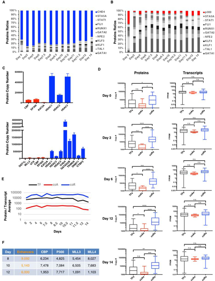
Large Excess of Co-Repressors and Limiting Amounts of Co-Activators in the Nucleus.

(A) Relative abundance of CHD4 protein compared to 10 erythroid TFs.

(B) Relative abundance of P300 protein compared to 10 erythroid TFs.

(C) Top panel: Quantitative imbalance between histone acetyltransferases (in red) and histone deacetylases (in blue). Bottom panel: Quantitative imbalance between co-activators (in red) and co-repressors (in blue).

(D) Left panel: Box plots depicting protein abundances (in copy numbers) of transcription factors (TFs, black), co-activators (coAs, red) and co-repressors (coRs, blue) at the indicated days. Right panel: Box plots depicting mRNA abundances (in FPKM) of TFs, coAs and coRs at the indicated days. For a list of TF, coA and coR, see Table S4. Two-tailed t-test: n.s. (non-significant), * p < 0.05. **p < 0.01. *** p < 0.001. **** p < 0.0001.

(E) Average of protein/transcript ratio for TFs, coAs and coRs at each day of differentiation.

(F) Estimated number of active enhancers compared to protein copy numbers of the indicated coAs in the nucleus at the indicated days.

See also Figure S4.

Figure 6.

The Nucleus is a Highly Repressive Environment with a Large Excess of Co-Repressors and Limiting Amounts of Unstable Co-Activators

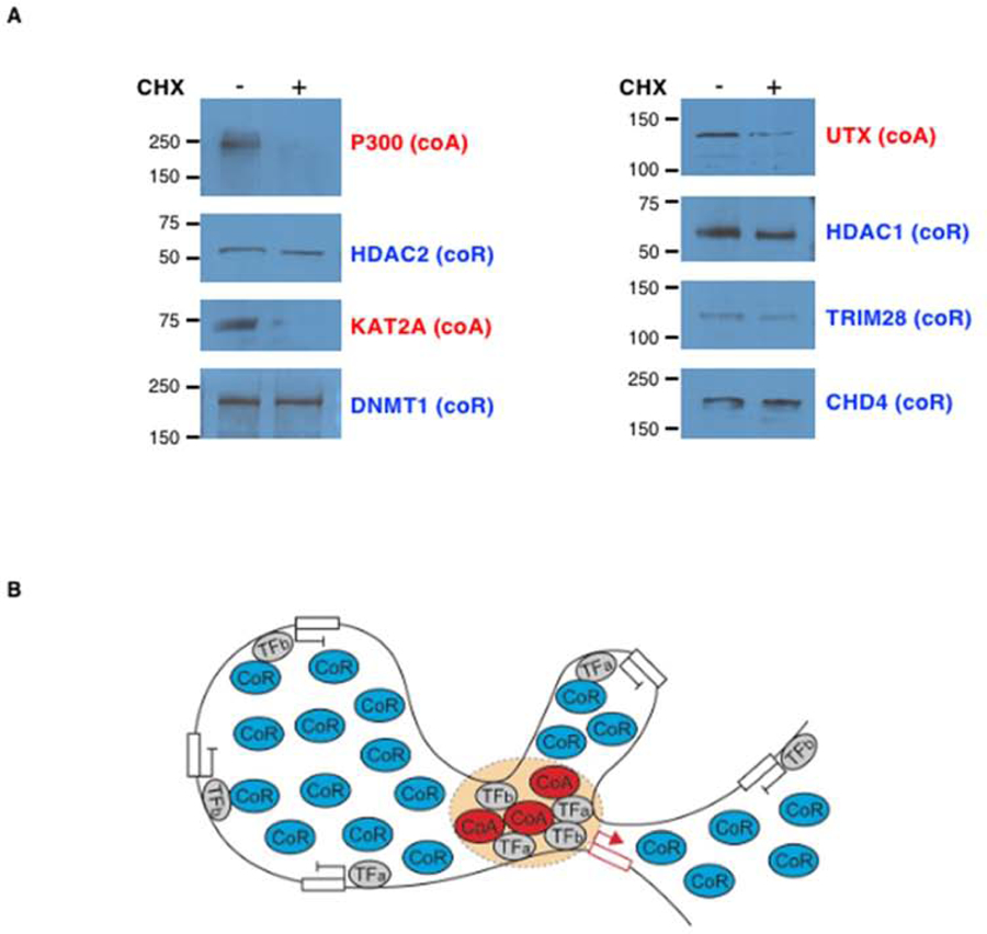
(A) Western blot analyses of nuclear extracts from erythroid cells (day 8) treated with cycloheximide (CHX) to inhibit translation or a vehicle control. Molecular masses (in kDa) are indicated on the left.

(B) Model of gene regulation in a highly repressive nuclear environment. In this model, the same TFs are able to interact with both coAs and coRs (Lambert et al., 2018). However, due to the scarcity of coAs in the nucleus, TFs must compete to recruit them, and they do so by creating an environment that allows multiple low affinity interactions as observed on enhancers (Farley et al., 2015; Hahn, 2018). In contrast, the high abundance of coRs increases their availability, which facilitates their recruitment to genes even in case of a small number of low affinity interactions with TFs.

TFs do not work in isolation, but instead upon binding to DNA, they form highly organized structures at enhancers to facilitate the recruitment of co-activators (Catarino and Stark, 2018). Thus, we asked whether co-activators are limiting or in excess compared to active enhancers. To estimate the number of active enhancers in erythroid cells, we performed ATAC-seq (Buenrostro et al., 2013) followed by HINT-ATAC (Li et al., 2019) at three time-points to identify TFs footprints within regions of open chromatin. These regions were then intersected with predicted enhancers from the GeneHancer database (Fishilevich et al., 2017). Since enhancers are characterized by specific histone modifications (H3K27ac and H3K4me1), we compared the number of identified enhancers with the number of molecules of co-activator enzymes responsible for these histone marks, including UTX (that demethylates H3K27), CBP and P300 (that acetylate H3K27) as well as MLL3 and MLL4 (that monomethylate H3K4). Interestingly, we found that the copy number of histone-modifying enzymes is on the same order of magnitude as the number of active enhancers (Figure 5F), suggesting a model whereby enhancer formation is dependent on co-activator molecules availability in the nucleus and enhancers must compete with each other to recruit rare and unstable co-activators in a highly repressive nuclear environment (Figure 6B).

Discussion

In this study, by measuring absolute abundances of TFs during the course of erythropoiesis, we uncovered major discrepancies between mRNA and protein levels for master regulators of hematopoiesis. Integration of protein stoichiometry data with mRNA measurements over time allowed us to establish a dynamic GRN, which revealed quantitative imbalances in TFs cross-antagonistic relationships that underlie lineage determination. Furthermore, comparing the abundances of coactivators and corepressors in the nucleus, we made the unexpected discovery that corepressors are dramatically more abundant, which has profound implications for understanding transcriptional regulation.

A central question in biology is how TFs control gene expression programs to direct cell processes such as lineage commitment. A pre-requisite for understanding the general principles of transcription is to define the key components (i.e. TFs and cofactors) quantitatively in absolute terms. Yet, despite years of studies, our knowledge of the copy number of TFs and cofactors in the nucleus is still limited. We also do not know the relative abundances of coactivators, corepressors and TFs. Here, through the use of targeted MS combined with spiked-in protein-specific standards, we offer an unprecedented view of the transcriptional machinery in the nucleus, providing an abundance scale for 103 major players in transcriptional regulation, including TFs, chromatin-modifying enzymes, coactivators, corepressors and subunits of the general transcriptional machinery at different stages of differentiation from HSPCs to erythroid cells. In addition to providing a quantitative scale for TFs in the nucleus, the protein data has changed our view on key aspects of erythroid differentiation. For instance, based on mRNA measurements, it was believed that the switch that occurs at the ProEB stage between GATA2 and GATA1 genomic binding to activate an erythroid gene program was due to GATA1 becoming more abundant than GATA2 at this stage (Katsumura et al., 2017). However, our protein data show that GATA1 is more abundant than GATA2 from the early stages of hematopoiesis. Thus, in contrast to the prevailing view, GATA2 is able to bind to its target genes despite an excess of GATA1, and the GATA2/GATA1 switch in genomic binding is likely to be mediated by a decrease in GATA2 protein level rather than competition with GATA1.

Another major finding is that in the nucleus, corepressors are highly abundant (e.g. >500,000 molecules per nucleus for CHD4) whereas coactivators such as P300 or CBP are comparatively very rare (<8,000 molecules per nucleus) with TFs being present at intermediate levels. This is consistent with the concept of “cofactor squelching” (also called “transcription interference”) (Meyer et al., 1989) which proposes that TFs compete for a limited number of cofactors in the nucleus. The squelching model was suggested 30 years ago based on reporter assays (Meyer et al., 1989) but had remained controversial due to the lack of data on TFs vs cofactors stoichiometry in cells (Schmidt et al., 2016). Our finding that coactivators are limiting compared to TFs in the nucleus provides strong support for a model whereby TFs compete with each other to recruit a limiting number of co-activators. Furthermore, this is compatible with emerging models of enhancer function that involve multiple weak interactions between coactivators, TFs and their genomic binding sites to achieve specificity in gene regulation (Farley et al., 2015; Hahn, 2018) (Figure 6B). In this regard, it is also interesting that the number of coactivator molecules and active enhancers are roughly equivalent in the nucleus, suggesting that the formation of active enhancers may depend on coactivator availability. Although the squelching model proposes passive repression as a mechanism for genes to remain inactive due to a lack of available coactivators, the high amounts of corepressors we detected indicate that the nucleus is a highly repressive environment with the recruitment of corepressors to target genes likely facilitated by their high abundance (Figure 6B). Consistent with this, NuRD has been shown to repress transcription of fetal ß-like globin genes in adult erythroid cells (Yu et al., 2019), and to suppress transcriptional noise during lineage commitment (Burgold et al., 2019). Based on these data, we propose that restricting the abundance of coactivators in a highly repressive nuclear environment is an important yet under-appreciated mechanism for concerted gene regulation during cellular processes such as cell fate decision, by ensuring only a limited number of genes can be expressed, and thus preventing high level co-expression of lineage-specific genes in multipotent progenitors.

Cell fate decisions are thought to be mediated through competition between LS-TFs that are co-expressed in multipotent progenitors (Huang et al., 2007; Palii et al., 2019). These regulatory relationships are typically represented by GRNs wherein LS-TFs inhibit each other within a stable progenitor state (Dore and Crispino, 2011; Gottgens, 2015). However, recent single cell analyses at the RNA (Zheng et al., 2018) and protein (Palii et al., 2019) levels have suggested that hematopoietic progenitors do not exist as a stable state but instead are gradually differentiating along lineage trajectories. Thus, there are uncertainties about how well previous GRN models capture lineage commitment. A major limitation of previous network models is that they did not incorporate quantitative changes in TF protein levels and instead used mRNA as a proxy for proteins. In contrast, we have integrated complementary measures on mRNA and protein abundances to build a temporal GRN of erythroid lineage commitment. Our model is unique in that it is both dynamic, allowing us to capture changes in regulatory relationships over time, and quantitative as it measures the strength of each regulatory relationship and the relative contribution(s) of different TFs to the regulation of their target genes (Figures 3 and 4 and Movie S1). Notably our model was able to accurately recapitulate the known cross-antagonisms between LS-TFs in their correct sequential order. Most importantly, the model revealed that these cross-antagonisms are quantitatively imbalanced and that these imbalances become more pronounced with time (Figure 3C,D). This suggests that lineage commitment can be quantified by measuring the imbalance between LS-TFs’ cross-antagonistic relationships. In summary, our GRN offers the first protein-based quantitative view of dynamic changes in gene regulatory relationships that underlie erythroid lineage commitment from HSPCs. We expect it will serve as a framework for integration of additional parameters such as other TFs/cofactors, post-translational modifications and/or genomic DNA binding data to allow for a more comprehensive understanding of transcriptional regulation during erythropoiesis.

Through the simultaneous measurement of RNA and proteins at multiple time points during erythropoiesis, we reveal major principles of transcriptional regulation that underlie lineage commitment. It is likely that the regulatory principles established here for erythropoiesis will be generally applicable to other cell types.

STAR Methods text

RESOURCE AVAILABILITY

Lead Contact

Further information and requests for resources and reagents should be directed to and will be fulfilled by the Lead Contact, Marjorie Brand (mbrand@ohri.ca).

Materials Availability

This study did not generate new unique reagents.

Data and Code Availability

All data generated during this study are available as follow:

RNA seq data have been deposited in the GEO database under GSE118537

ATAC seq data have been deposited in the GEO database under GSE137446

iTRAQ protein data has been deposited in ProteomeXchange via MassIVE under the identifier PXD017490.

URL: https://massive.ucsd.edu/ProteoSAFe/static/massive.jsp

SRM protein data have been deposited into The Peptide Atlas SRM Experiment Library (PASSEL) under the identifier PASS01454.

URL: http://www.peptideatlas.org/PASS/PASS01454

The original Western blots for Figure S1B and E, Figure 6A and Figure S3 are available in Mendeley.

http://dx.doi.org/10.17632/75vs43ydbf.1

EXPERIMENTAL MODEL AND SUBJECT DETAILS

Hematopoietic stem/progenitor cells isolation

Umbilical cord blood from female and male donors was obtained from Canadian Blood Services “Cord Blood for Research program” (CBR-2014-001). CD34 ⁺ hematopoietic stem/progenitor cells were isolated as previously described (Palii et al., 2011a) with some modifications. First, CD34⁺ cells were enriched from fresh cord blood by negative selection using the RosetteSep Human Cord Blood CD34 Pre-Enrichment Cocktail (STEMCELL Technologies cat#15631), followed by Ficoll density gradient and CD34 positive selection using the EasySep Human CD34 Positive Selection Kit (STEMCELL Technologies cat#18096) according to the manufacturer’s instructions. Purified cells were analyzed by FACS for CD34 expression using the PE Mouse Anti-Human CD34 antibody (BD Pharmingen, cat# 555822) and either cryopreserved in 10% DMSO or cultured directly as described below. All procedures were approved by the Ottawa Health Science Network Research Ethics Board (2007804-01H)

Human erythropoiesis ex vivo culture and cell harvest

Two biological replicates of the time-series were performed. CD34⁺ cells (63×10⁶ cells for replicate 1 and 45×10⁶ cells for replicate 2) were differentiated towards the erythroid lineage using a 4-step protocol (Giarratana et al., 2005; Palii et al., 2011a). The first step (day 0 to day 11) consists of growing CD34⁺ cells in serum-free IMDM medium supplemented with 1% penicillin/streptomycin, 4×10⁻³ M L-glutamine, 40 ug/ml inositol, 10 ug/ml folic acid, 1.6×10⁻⁴ M monothioglycerol, 90 ng/ml ferrous nitrate, 900 ng/ml ferrous sulfate, 20% albumin-insulin-transferrin (BIT), also containing the following cytokines: 10⁻⁶ M hydrocortisone (HC), 100 ng/ml stem cell factor (SCF), 5 ng/ml interleukin 3 (IL-3) and 3 IU/ml erythropoietin (EPO) for 8 days followed by 3 days in supplemented IMDM medium containing only SCF and EPO. For the second step (day 12 to day 14), cells were co-cultured on a layer of stromal MS-5 cells in the supplemented IMDM medium containing only EPO. For the third step (day 15 to day 18), cells were co-cultured on a layer of MS-5 cells in the supplemented IMDM medium with no cytokines. For the fourth step (day 19 to day 24), cells were co-cultured on a layer of MS-5 cells in the supplemented IMDM medium in the presence of 10% fetal bovine serum. Every second day, cells were counted and monitored for viability (trypan blue exclusion of dead cells), cell surface expression of CD34 (CD34-PE, BD Pharmingen, cat# 555822), CD36 (CD36-PE, BD Pharmingen, cat# 555455), CD71 (CD71-FITC, Beckman Coulter, cat# IM0483U), GPA (CD235a-PE, BD Pharmingen, cat# 555570) and LDS751 (Molecular Probes, cat# L7585) by FACS and hemoglobin production (benzidine staining). Cells were harvested at the indicated intervals during the course of differentiation and cryopreserved in their respective culture media supplemented with 10% DMSO.

Murine bone marrow stromal MS-5 cells were obtained from DSMZ (cat#ACC 441; RRID:CVCL_2128) and cultured as follow. Cells are seeded at 2 million cells/80 cm² (for a 10 cm dish) in alpha-MEM medium containing ribo- and deoxyribonucleosides (StemCell Technologies, cat# 36450) supplemented with 10% FBS, 2mM L-glutamine, 2 mM sodium pyruvate and 1% penicillin/streptomycin. Confluent cultures are split 1:3 every third day using 0.05% Trypsin/EDTA

Human embryonic kidney 293T cells were obtained from ATCC (cat#CRL-3216; RRID:CVCL_0063) and cultured as follow. Cells are seeded at 1 million cells/80 cm² (for a 10 cm dish) in Dulbecco’s Modified Eagle’s Medium (DMEM)/High Glucose (HyClone, cat# SH30243.01) supplemented with 10% FBS, and 1% penicillin/streptomycin. Confluent cultures are split 1:5 every two to three days using 0.05% Trypsin/EDTA.

All cell lines are regularly tested for mycoplasma contamination and tested negative.

METHOD DETAILS

Giemsa staining

Cells were harvested, cytospun and fixed in methanol for 5 min prior to staining with 1/20 diluted Giemsa solution (SIGMA cat# GS500) for 15 min, followed by 3 washes of 5 min each in deionized water, according to the manufacturer’s instructions.

RNA extraction and high throughput sequencing

For each biological replicate, total RNA was isolated on days 0, 2, 4, 6, 7.5, 8, 8.5, 10, 10.5, 11, 11.5, 12, 14 and 16 of erythroid differentiation using the RNeasy mini extraction kit (Qiagen, cat# 74104), including a DNase I digestion step. After RNA extraction, quality control was performed with RNA 6000 Nano kit (Agilent cat# 5067–1511). mRNA enrichment was performed using the NEBNext Poly(A) mRNA Magnetic Isolation Module (NEB cat#E7490S/L) and libraries were prepared using the KAPA Stranded RNA-seq Library Preparation Kit (KAPABiosystems cat#KR0934) with two biological replicates per library. Paired-end sequencing was performed on an Illumina HiSeq 2000.

RNAseq analysis

For each biological replicate, fastq files were aligned to the human reference genome hg38 with RefSeq annotations using Hisat2 (Kim et al., 2015). The resulting .sam files were transformed into .bam files with SAMtools (Li et al., 2009). The reads were counted using the featureCounts (Liao et al., 2014) function from the R package Rsubread, specifying the same .gtf file used to build the Hisat2 index and default parameters. Differentially expressed genes were identified with the R package DESeq2 (Love et al., 2014). Genes with adjusted p-value below 0.05 were considered statistically significant. For visualization the data was normalized to FPKMs. Principal Component Analysis was done with the R function prcomp using the log(1+FPKM) transformed data.

Nuclear protein extraction and relative quantification using iTRAQ

Fifteen million cryopreserved cells at days 0, 2, 4, 6, 8, 10, 12 and 14 of erythroid differentiation were thawed and resuspended in serum-free IMDM medium supplemented with 1% penicillin/streptomycin, 4×10⁻³ M L-glutamine, 40 ug/ml inositol, 10 ug/ml folic acid, 1.6×10⁻⁴ M monothioglycerol, 90 ng/ml ferrous nitrate, 900 ng/ml ferrous sulfate, 20% albumin-insulin-transferrin (BIT). After thawing, the cells were washed twice with ice-cold PBS, resuspended in ice-cold Swelling Buffer (10mM HEPES pH7.9, 1.5mM MgCl₂, 10mM KCl, 0.1% (v/v) NP-40, protease inhibitor cocktail) and incubated on ice for 30 min. During incubation, cells were vortexed every 5 min to allow cell lysis. Nuclei were then pelleted by centrifugation at 1,500 rpm (4°C) for 5 min, washed twice with ice-cold PBS and resuspended in RIPA Buffer (50mM HEPES pH7.9, 1mM MgCl₂, 150mM NaCl, 0.5% (w/v) Na deoxycholate, 1% (v/v) NP40, 0.1% SDS) containing 50 ng/µl Benzonase (Millipore, cat# 70746) and protease inhibitor cocktail at room temperature (RT). Samples were vortexed for 5 min at RT and incubated for 20 min at 37°C on a Thermomixer (14,000 rpm) followed by 5 min vortexing at RT. Nuclear extracts were recovered by centrifugation at 14,000 rpm for 15 min, snap frozen in liquid nitrogen and stored at −80°C. Nuclear protein extracts were prepared from cells on days 0, 2, 4, 6, 8, 10, 12, and 14 of erythroid differentiation. Extracted protein concentrations were measured using the bicinchoninic acid assay (BCA; Thermo Scientific). Equal protein amounts were reduced with 5mM dithiothreitol, alkylated with 10mM iodoacetamide, and precipitated with chilled 100% acetone to remove detergent. Precipitated proteins were resuspended in iTRAQ Dissolution Buffer (AB Sciex) and digested into solution with Lys-C for 3 h (1:200 w:w, 37C; Thermo Scientific) followed by Trypsin overnight (1:50 w:w; 37C; Thermo Scientific). Volatile liquids were removed by evaporation, and peptides were resuspended in iTRAQ Dissolution Buffer and labeled with 8-plex iTRAQ reagents (AB Sciex) for 2 h at room temperature with constant agitation. The labeling reaction was quenched with 1M Tris, pH 8.0, and samples were combined and volatile liquid was evaporated. Labeled peptides were resuspended in 1% acetonitrile, acidified with formic acid, and purified using C18 reversed-phase chromatography (1cc 100mg cartridges; Waters). Purified peptides were separated into 24 fractions using isoelectric focusing off-gel electrophoresis (Agilent), and ampholytes removed by tC18 reversed-phase chromatography (100mg 96-well plate; Waters) followed by mixed cation exchange chromatography (30um uElution 96-well plate; Waters). Purified peptides were separated by online nanoscale HPLC (EASY-nLC1000; Thermo Scientific) with a C18 reversed-phase Picochip nanospray column pre-packed 10.5cm with ReproSil-Pur C18-AQ 3um 120A (New Objective) over an increasing 90 min gradient of 5–35% Buffer B (100% acetonitrile, 0.1% formic acid) at a flow rate of 300nl/min. Eluted peptides were analyzed with a Q Exactive HF Hybrid Quadrupole-Orbitrap mass spectrometer (Thermo Scientific) operated in data dependent mode, with the Top15 most intense peptides per MS1 survey scan selected for MS2 fragmentation by higher energy collisional dissociation (HCD). MS1 scans were performed in the Orbitrap at a resolution of 60,000 at m/z 400, with an automatic gain control (AGC) target of 3e6 ions and a maximum injection time of 20ms. MS2 scans were analyzed in the Orbitrap at a resolution of 15,000, with an AGC target of 1e5 and a maximum injection time of 45ms. Due to the iTRAQ label, a fixed first mass of 100 m/z was used for MS2 scans, along with a normalized collision energy of 30 and an isolation window of 1.2 m/z. Peptide match was not used, and dynamic exclusion was set to 30 s (+/−15 ppm). Raw output data files were searched against the Uniprot human protein database (12–2015 release) using X!Tandem and Comet (Craig and Beavis, 2004; Eng et al., 2013) to identify peptide sequences. A reverse sequence database was appended to assist in determining error. Resulting data were combined using iProphet, and probabilities for correct identification were determined by Peptide prophet, iProphet, and Protein prophet (Keller et al., 2002; Nesvizhskii et al., 2003; Shteynberg et al., 2011). iTRAQ quantification was performed using Libra (Pedrioli et al., 2006). See Table S1.

iTRAQ data clustering analysis

iTRAQ data was clustered using k-means clustering with the R function kmeans, with centers=8 and default parameters. Gene Ontology (GO) analysis of the different clusters was done using Metascape (Zhou et al., 2019) with the option Express Analysis. See Table S2.

Construction of an Erythroid protein database

Day 8 nuclear protein extracts (86 µg) were reduced with 5mM dithiothreitol, alkylated with 25mM iodoacetamide, and digested with Lys-C for 3 h (1:200 w:w, 37C; Thermo Scientific) followed by Trypsin overnight (1:25 w:w, 37C; Thermo Scientific). Peptides were acidified with formic acid, purified using C18 reversed-phase chromatography (1cc 100mg cartridges; Waters), and separated into 24 fractions using isoelectric focusing off-gel electrophoresis (Agilent). Ampholytes were removed by tC18 reversed-phase chromatography (100mg 96-well plate; Waters) followed by mixed cation exchange chromatography (30um uElution 96-well plate; Waters). Purified peptides were separated by online nanoscale HPLC (EASY-nLC II; Proxeon) with a C18 reversed-phase column packed 25cm (Magic C18 AQ 5um 100A) over an increasing 60 min gradient of 5–35% Buffer B (100% acetonitrile, 0.1% formic acid) at a flow rate of 300nl/min. Eluted peptides were analyzed with an Orbitrap Elite mass spectrometer (Thermo Scientific) operated in data dependent mode, with the Top20 most intense peptides per MS1 survey scan selected for MS2 fragmentation by rapid collision-induced dissociation (rCID) (Michalski et al., 2012). MS1 survey scans were performed in the Orbitrap at a resolution of 240,000 at m/z 400 with charge state rejection enabled, while rCID MS2 was performed in the dual linear ion trap with a minimum signal of 1000. Dynamic exclusion was set to 15 s (+/− 10 ppm). Raw output data files were searched against the Uniprot human database (03–2015 release) using X!Tandem and Comet (Craig and Beavis, 2004; Eng et al., 2013) to identify peptide sequences. A reverse sequence database was appended to assist in determining error. Resulting data were combined using iProphet, and probabilities for correct identification were determined by Peptide prophet, iProphet, and Protein prophet (Keller et al., 2002; Nesvizhskii et al., 2003; Shteynberg et al., 2011). Xpress was used to determine the summed peak area for each peptide (Han et al., 2001).

Construction of the Erythroid SRM TF Atlas

We created a list of 168 TFs with known and/or expected roles in transcriptional regulation during erythropoiesis. Proteotypic, fully tryptic peptides with the highest summed MS1 peak areas were selected from the erythroid protein database for all proteins of interest. In addition, selected peptides were a minimum of 7 amino acids in length and lacked features that may be incompatible with SRM analysis, namely ragged ends or missed cleavages. Where possible, Cys-containing peptides, peptides containing potentially modified residues (e.g., Met, Ser, Thr, Tyr, N-terminal Gln, Asn-Gly, Gln-Gly) and sequences that could affect trypsin digestion efficiency or peptide stability were also avoided. For proteins not found in our database, or to supplement our identified peptides, the SRM Atlas (Kusebauch et al., 2016) was used with a preference for peptides validated on an Agilent triple quadrupole mass spectrometer. In the few instances where a protein of interest was not present in our erythroid protein database and there were no corresponding peptides in the SRM Atlas, we relied upon Peptide Atlas (Deutsch et al., 2015), or prediction software (Fusaro et al., 2009)). In sum, we derived 5% of peptides using these approaches: 3% from Peptide Atlas, and 2% from ESP Predictor. SIL peptides (Lys-[13C6, 15N2] or Arg-[13C6, 15N4]) were synthesized for all proteins (716 peptides; PEPotec). Transitions and collision energy values were imported from the SRM Atlas, when available, or derived empirically (MacLean et al., 2010). Next we determined which of these peptides displayed the highest interference-free signal intensities in solvent and when added to erythroid cell extracts. In addition, the peptides were screened for their ability to produce a linear dose response. After screening 716 SIL peptides corresponding to 168 TFs, we were left with 411 peptides corresponding to 150 TFs (3–4 transitions per peptide and 1–4 peptides per protein) that satisfied these requirements (Table S3). These SIL peptides were used as standards for confident peptide identification during SRM and to optimize SRM assays. The concentration of SIL peptides used in the final time course measurements was matched to that detected in day 8–12 erythroid nuclear extracts.

Nuclear protein extraction and sample preparation for SRM analyses

Fifteen million cryopreserved cells at days 0, 2, 4, 6, 7.5, 8, 8.5, 10, 10.5, 11, 11.5, 12, and 14 of erythroid differentiation were thawed and washed using IMDM supplemented medium. Cells were then washed in ice-cold PBS buffer, resuspended in ice-cold Swelling Buffer (10 mM HEPES pH7.9; 1.5 mM MgCl₂; 10 mM KCl; 0.1% (v/v) NP40; protease inhibitor cocktail) and incubated on ice for 30 min. During incubation, cells were vortexed every 5 min to allow cell lysis. Nuclei were then pelleted by centrifugation for 5 min at 1,500 rpm (4°C) and resuspended in 1 vol. of 37°C pre-heated Extraction Buffer 1 (50 mM HEPES pH7.9; 1 mM MgCl₂; 150 mM NaCl; 0.5% Na deoxycholate; 50 ng/µl Benzonase Millipore, cat# 70746; protease inhibitor cocktail) prior to incubation at 37°C on a Thermomixer (14,000 rpm) for 15 min. Proteins were extracted first by 6 passages through a 27 ½ gauge needle prior to addition of 1 vol. of 37 °C pre-heated Extraction Buffer 2 (50 mM HEPES pH7.9; 150 mM NaCl; 9.5% Na deoxycholate; 1 mM EDTA; protease inhibitor cocktail). The mixture was heated at 70°C for 5 min and proteins were extracted further by 6 passages through a 27 ½ gauge needle prior to incubation at 40 °C on a Thermomixer (14,000 rpm) for 15 min. Nuclear extracts were recovered by centrifugation at 13,000 rpm for 15 min and snap frozen. Extracted protein concentrations were measured using the BCA assay (Thermo Scientific). Equal protein amounts were denatured by boiling at 100°C for 4 min, cooled and reduced with 5mM dithiothreitol, alkylated with 25mM iodoacetamide, and digested with Lys-C for 3 h (1:200 w:w, 37C; Thermo Scientific). Samples were diluted to reduce sodium deoxycholate concentration to below 1%, and digested with Trypsin overnight (1:25 w:w, 37C; Thermo Scientific). Concentration-matched isotopically heavy peptide standards were added to erythroid peptide samples after overnight digest. To remove sodium deoxycholate and prepare peptides for purification, samples were acidified with an equal volume of cold 1% trifluoroacetic acid. Acidified supernatants were subsequently purified by mixed cation exchange chromatography (30um uElution 96-well plate; Waters).

Sample Processing for SRM

SRM was performed on an Agilent 6490 triple quadrupole mass spectrometer, equipped with a chip cube interface. Peptides were separated by online HPLC (1260 Infinity; Agilent) with a reversed-phase microfluidics HPLC chip (160nL trap; Agilent) over an increasing 60min gradient of 3–25% acetonitrile. Optimized transitions were acquired in dynamic MRM mode, with a 5 min retention time window, using MS1 wide and MS2 unit resolutions. Collision cell accelerator voltage was set to 5V, and cycle times were set to yield a minimum dwell time of 12ms. Raw data was processed using Skyline (MacLean et al., 2010) and peaks were manually verified. Light-to-heavy ratios were calculated from peak area values. Only measurements determined to be within the linear range of quantification for the mass spectrometer were used for subsequent analyses.

Technical considerations regarding peptide quantification

In this study we used SIL peptides and SID-SRM to quantify target proteins. A limitation of peptide-based protein quantification is that it may not reflect the variability of abundances for a given protein. This can result from the presence of isoforms or post translationally modified forms of the protein, and/or inefficient protein digestion during sample processing. This issue is particularly relevant when only a single peptide is used for quantification. One way to assess the variability of protein abundance would be to use recombinant, isotopically labeled, full length protein standards, instead of synthetic peptides, for each target protein (Simicevic et al., 2013). These protein standards would be quantified, and spiked-into the biological samples prior to protein digestion, thus controlling for potential inaccuracies in quantification due to inefficient digestion. This approach provides the opportunity to use all detectable, interference-free proteotypic peptides for protein quantification which could reveal variability in protein abundances. The main challenges of implementing this approach are the production of the recombinant protein standards, the development of the SRM assays for all detectable peptides, and the increased sample requirement and instrument time needed to acquire the data.

Quantification of proteins using Western blots

For orthogonal quantification of TRIM28, PU.1, and GFI1B, we used purified GST to quantify GST-tagged protein standards corresponding to these TFs. We then used the protein standards to quantify the endogenous transcription factors, as described below.

Recombinant Glutathione S-Transferase (GST) protein was expressed from the pGEX-4T vector transformed into E. coli BL21 cells (GE Healthcare). Following overnight growth, protein expression was induced with 2mM Isopropyl-β-D-thiogalactopyranoside (IPTG) for 2 h at 37C. Cells were lysed with 1% Triton X-100, sonicated, and incubated with glutathione-sepharose beads (GE Healthcare). Captured protein was washed 3 times with PBS and eluted with 10mM glutathione. Glutathione was subsequently removed by dialysis against 50mM Tris pH 8 overnight. Purified GST protein was separated by SDS-PAGE and visualized by SimplyBlue SafeStain (Life Technologies) to ensure a single product of correct size. GST protein was quantified in triplicate using the BCA assay.

Expression clones for GST-tagged versions of TRIM28, PU.1, and GFI1B were obtained from DNASU (Seiler et al., 2014) and in vitro transcribed/translated using the 1-Step Human Coupled IVT kit (Life Technologies) according to manufacturer’s protocol. These proteins were then visualized by Western blotting together with serial dilutions of purified GST protein, and quantified by image analysis (Image Lab; Bio-Rad). The concentration of TFs in erythroid nuclear extracts was determined by comparison to the quantified protein standards by Western blotting and image analysis.

Gene Regulatory Network modeling

For a core set of factors (ELF1, ERG, FLI1, GATA1, GATA2, GFI1B, KLF1, NFE2, RUNX1, TAL1, SPI1), possible regulatory links were obtained from the literature (Dore and Crispino, 2011; Gottgens, 2015; Sive and Gottgens, 2014). For three genes (E2F2, HXB4, KLF3), literature evidence was insufficient to suggest regulatory links. For each of these three genes, we computed correlations between the RNA expression of the gene and the protein expression of all other genes in the network. The three other genes with highest correlation were posited to be possible activators, and the gene with most negative correlation was posited to be a possible repressor. This network of possible activators and repressors was further refined by fitting ordinary differential equation models to the quantitative expression data.

Given a gene X, let x denote our modeled (or predicted) RNA expression of gene X, in units of FPKM. Let A_i(t) denote the observed protein expression of the i^th activator of gene X, and R_j(t) the observed protein expression of the j^th repressor of gene X, both in units of fmol/µg. We model the RNA transcription of X as

$$\frac{dx}{dt}=\frac{{\sum }_{i=1}^{\left[n_A\right]}{k}_i{A}_i}{1+{\sum }_{j=1}^{n_R}{k}_{n_A+j}{R}_j}-\lambda \text{x}$$

where k_i and are constants to be determined, is the number of activators considered for X and n_R is the number of repressors considered for X. Given an initial condition, x(0), values for the A_i and R_i as a function of time, and values for the regulatory and decay parameters, the above ordinary differential equation (ODE) can be solved numerically over any finite time interval, producing predicted values x(t, k, λ). We used a Runge-Kutta 7(8) method to calculate such trajectories.

The values for for A_i and R_j as a function of time are obtained by interpolation from the observed SRM (protein) values, using a cubic spline smoothing from the GSL libraries (Galassi).

Given also observed RNA expression values for gene X, O(t_i) at observation times t₁, t₂, …, t_m, agreement between predicted and observed expression values can be quantified using the objective function

$$G\left(x\right)={{\sum }_{i=1}^m\left(O\left(t_i\right)-x\left(t_i,k,\lambda \right)\right)}^2$$

To find regulatory and decay parameters, we sought to minimize the objective function, subject to the constraints that all parameters need to be positive and decay rate has to be larger than 16.6 day⁻¹.

The minimum of the objective function was computed using a Simplex method from the GSL libraries. To explore the parameter space we choose random initial parameters between 0 and 500 for the k’s, and between 16.6 day⁻¹ and 500 day⁻¹ for the λ with stop conditions either error below 1e-04 or a maximum of 2000 iterations. With a total of 128 random initial conditions. Out of the 128 iterations, the parameter set that gives the smallest values in the objective function were selected.

Gene Regulatory Network display

For activators, the transparency score of the link representing A_i activating X at time t is

$$\frac{k_i{A}_i\left(t\right)}{ma{x}_{i,t}{k}_i{A}_i\left(t\right)}$$

Links with transparency score below 0.1 at a certain time are not displayed. Links with transparency scores between 0.1 and 1 are increasingly opaque, and links with scores greater or equal to 1 are fully opaque. For repressors, the transparency score of the link representing R_i repressing X is log₂(1+K_iR_i). The thickness of a link from a regulator (activator A_i or repressor R_i) to gene X is proportional to log(1+K_i). See Figure 3.

Intersection of GRN putative links with published ChIP-seq data:

Published ChIP-seq data for ERG (GSM1097879), FLI1 (GSM1097880), GATA1 (GSM1278240, GSM1067274), GATA2 (GSM1097883), KLF1 (GSM2575041-GSM2575049, GSM1067275), PU.1 (GSM1816089, GSM1816090), RUNX1 (GSM1816092, GSM1097884, GSM1816091) and TAL1 (GSM1278241, GSM1097881, GSM1816083) corresponding to CD34⁺ HSPC (Day 0–2) or ProEB (Day 10) stages (Beck et al., 2013; Huang et al., 2016; Norton et al., 2017; Pinello et al., 2014) were downloaded from NCBI GEO and analyzed as follow. Raw fastq data was trimmed for low quality bases using trimmomatic (version 0.38) (Bolger et al., 2014), and mapped to the human genome (hg38) using bowtie-2 (Langmead and Salzberg, 2012). Aligned reads were filtered for multiple mapping using a mapping quality filter (Q20) and the filtered alignments were sorted (using samtools version 1.9 (Li et al., 2009)) and used for calling peaks. Peaks were called using MACS2 (version 2.1.2) (Zhang et al., 2008), with a peak enrichment cut-off filter of P = 0.05. The peaks were filtered against ENCODE blacklist (Amemiya et al., 2019) for human genome using bedtools v2.27.1. For each sample, an appropriate Input sample from the same stage of development was used as a control. Genome coverage files were created using deepTools2 suite (bamCoverage) (Ramirez et al., 2016). The identified ChIP-seq peaks were overlapped with GeneHancer (v4.4) (Fishilevich et al., 2017) elements (promoters and enhancers) using bedtools. This filtered list was then intersected with putative links from the GRN model at day0 or day2 (HSPCs) or day 10 (ProEB) to identify possible direct interactions between TFs and target genes (TGs). Based on this data, we classified TF–TG pairs as either “interacting” or “not interacting” and calculated the percentage of regulatory links that could be explained by direct TF binding. See Table S5.

Lentivirus preparation and infection

Lentiviral particles expressing shRNA sequences against GATA2 (5’-CCAGACGAGGTGGACGTCTTCTTCAATCA-3’), GATA1 (5’-GATCCCCGAAGCGCCTGATTGTCAGTTTCAAGAGAACTGACAATCAGGCGC TTCTTTTTGGAAA-3’), TAL1 (5’- CTTACTCTAGGAGGCGGAC-3’), and KLF1 (5’- CCGGACACACAGGATGACTTCCTCAAGTG −3’) were prepared as previously described (Palii et al., 2011a). Specifically, HEK293T cells were transfected with the pMD2.G envelope vector (Addgene #12259), the psPAX2 packaging vector (Addgene, #12260) and one of the following shRNA expression lentiviral vectors: GATA2 shRNA Lentivector Target a (Abm #i008537a), pLVUTHshGATA1-tTR-KRAB (Addgene #11650), pBLOCK-it6-DEST (sh Tal1) (Palii et al., 2011b) or KLF1 shRNA Lentivector Target a (Abm #i011644a), using calcium phosphate precipitation. Lentiviral particles were harvested, concentrated by ultracentrifugation (50,000 g for 2h) and used to infect cells at the day 8 time-point with a MOI of 20. Lentiviral infection was repeated 24h later in the same conditions. Cells were harvested 24h after the last infection and used for RNA extraction.

ATACseq, HINT-ATAC and estimation of the number of active enhancers.

ATAC-seq was performed as previously described (Buenrostro et al., 2013; Hay et al., 2016) for cells at days 8, 10 and 12. Briefly, 75000 cells per technical replicate per sample per timepoint were lysed in cold lysis buffer, nuclear pellets were obtained after 10 min centrifugation at 4°C at 500G and resuspended in 50ul of tagmentation mix (FC-121–1030, Illumina), then incubated for 30 min at 37°C. DNA was purified using the Qiagen MinElute columns (28004, Qiagen). Tagmented DNA was indexed with custom primers using NEB Next High-Fidelity 2x PCR Master Mix (M0541S, NEB) and purified with Qiagen PCR Cleanup Kit (28104, Qiagen). Samples were multiplexed sequenced on a next generation sequencing platform using the NextSeq® 500/550 High Output Kit v2 (75 cycles; FC-404–2005, Illumina) using paired-end reads. For data analysis, the fastq data was mapped onto the human genome (hg38) using bowtie1.0 (Langmead et al., 2009) with the following parameters: --chunkmb 256 –phred-quals 33 –m 2 –best –strata –maxins 400. The mapped bam files were used to call narrow peaks using MACS2 with the version 2.1.2 docker image of macs https://hub.docker.com/r/fooliu/macs2

In preparation for running HINT-ATAC, all peaks which mapped to non-canonical chromosomes (chr1–22, X, Y, M) were eliminated (“cleaned”) and a bam index was built for each bam file using samtools version 1.8. HINT was then run from the regulatory genomics toolkit, version 0.12.3 (http://www.regulatory-genomics.org/hint/introduction/) on the indexed bam file, and the cleaned peaks file rgt-hint footprinting --atac-seq --organism=hg38 $(BAM) $(PEAKS) Putative enhancer and promoter regions from GeneHancer 4.1.1. were identified for all tissues, and the Bioconductor GenomicRanges package was used to calculate the intersection of macs2 narrowpeaks and hint-called ATAC-seq footprints with the sets of enhancers. See Figure 5F.

Cycloheximide treatment and nuclear protein extraction

Erythroid cells at day 8 were treated with 1µg/mL of cycloheximide or DMSO vehicle control for 3h. Cells were washed twice with ice-cold PBS, resuspended in ice-cold Swelling Buffer (10mM HEPES pH7.9, 1.5mM MgCl₂, 10mM KCl, 0.1% (v/v) NP-40, protease inhibitor cocktail) and incubated on ice for 30 min. During incubation, cells were vortexed every 5 min to allow cell lysis. Nuclei were then pelleted by centrifugation at 1,500 rpm (4°C) for 5 min, washed twice with ice-cold PBS and resuspended in RIPA Buffer (50mM HEPES pH7.9, 1mM MgCl₂, 150mM NaCl, 0.5% (w/v) Na deoxycholate, 1% (v/v) NP40, 0.1% SDS) containing 50 ng/µl Benzonase (Millipore, cat# 70746) and protease inhibitor cocktail at room temperature (RT). Samples were vortexed for 5 min at RT and incubated for 20 min at 37°C on a Thermomixer (14,000 rpm) followed by 5 min vortexing at RT. Nuclear extracts were recovered by centrifugation at 14,000 rpm for 15 min, snap frozen in liquid nitrogen and stored at −80°C before Western blot analysis.

QUANTIFICATION AND STATISTICAL ANALYSIS

Absolute quantification of transcription factors by SRM

Absolute quantification was achieved in two ways: The first approach (71 proteins) is based on stable isotope dilution (SID) in which peptide abundance is determined by comparison of selected transition peak areas for each peptide to those of its corresponding SIL peptide. The second approach (34 proteins) is a label free method in which SID is used to determine the concentration of a set of 17 “anchor” proteins, and standard curves based on transition peak areas from the two highest intensity peptides per anchor protein and their concentrations are then used to estimate the concentrations of the target proteins (Ludwig et al., 2012).

For SID, isotopically light internal standard (IS) peptides (Gerber et al., 2003) were used to quantify our SIL standard peptides. This approach enabled a significant time, cost and resource savings versus using isotopically heavy IS peptides for assay development and direct quantification in the biological matrix. Peptides that showed the highest interference-free intensity were selected for commercial synthesis (AQUA; Thermo Scientific). IS peptides were >97% pure and were quantified by amino acid analysis. For SRM quantification, the peak areas for the two most intense, interference-free transitions were summed together. Additional transitions were used to confirm correct peak identification. Dose-response curves were generated for each IS peptide at abundances ranging from 10 amol to 500 fmol (Data S1B). Quantification of the SIL peptides was achieved by measuring transition intensities from serial dilutions of the peptides and then plotting the corrected peak areas onto the corresponding IS dose-response curve. The technical variability as assessed by repeated quantifications of these SIL peptides is reflected by a mean coefficient of variation (CV) of 0.224 (Data S1D). The light-to-heavy ratios calculated for the erythroid differentiation time course were used to convert these SIL standard abundance measurements into endogenous protein abundances. Peptide-based protein abundances were averaged in cases where more than 1 peptide/protein was quantified.

For label free absolute quantification, the following criteria were used to select “anchor” proteins for the standard curves: (i) IS dose-response regression line was linear between 0.1–500 fmol with an R2>0.98; or (ii) IS dose-response regression line was linear between 1–500 fmol with an R2>0.98 and a slope>0.8; or (iii) IS dose-response regression line was linear between 1–500 fmol with an R2>0.95 and the peptide was included based on (i) or (ii) in another replicate. All peptides satisfying at least one of these criteria were weighted equally when preparing the standard curve. Peak areas were calculated by summing the two most intense interference-free transitions per peptide, and averaging these values for the two highest intensity peptides per protein. Linear regression was used to fit a standard curve to the above values, and to estimate the unknown concentrations of endogenous proteins using their measured transition peak area values (Data S1C). The limits of quantification (LOQ) for anchor proteins is provided in Table S4.

SRM measurements obtained as described above produced biological duplicate values in units of fmol/µg of protein for each protein at each time point. Values outside the linear range of quantification were removed. Zeros were added to indicate select measurements that did not produce a detectable signal in the mass spectrometer. This was based on the assumption that neighboring values would either decrease as they approached the missed measurement, or increase from the missed measurement as the time course progressed. In addition, the expression trend of the replicate biological measurement was used to inform this decision. The two replicates were combined by the following steps, to produce a single abundance value for each gene at each time point. First, if both replicates had a valid measurement, the two were averaged. If only one replicate had a valid measurement, it alone was taken as the representative value. If neither replicate had a valid measurement, the value was marked as missing. Second, missing values were filled in by linear interpolation where possible. For each missing value (say on day y), we sought the latest non-missing value prior (say on day x) and the earliest non-missing value later (say on day z). If such days could be found, then the abundance at day x was filled in with (z-y)/(z-x) times the abundance at day x, plus (y-x)/(z-x) times the abundance at day z. This interpolation rule was not applied to genes ETO2, MLL1 and SPT16, as visual inspection suggested there were too many missing values and/or not clear enough of a trend in abundance for interpolation to be meaningful. This left only one gene, BACH1, with a missing value at our final time point, which we filled in as zero consistent with BACH1’s general trend towards decreasing expression. See Table S4. Some analyses, such as the GRN modeling (Figure 3), used these numbers. For other analyses (Figures 2, 4, 5 and Data S2), we wanted to express protein abundance in units of protein copy number per nucleus To obtain these numbers, we multiplied by 4420.25799, which comes from the following considerations: (1) There are 6.022140857e+8 molecules per fmol. (2) Across all samples, we extracted an average of 7.3426 µg protein per million nuclei. By comparing quantifications of the same proteins at the same time points between our two biological replicates, we observe a mean CV of 0.3106 and a Pearson correlation coefficient of 0.86 between log-transformed abundances (Data S1 E–F).

Comparison of protein abundances for TFs, coAs and coRs

For this analysis, TFs were defined as proteins that bind to DNA in a sequence-specific manner and regulate transcription. CoAs and coRs were defined in the strictest sense as proteins that have been shown to be recruited to genomic locations by TFs and to respectively activate or repress transcription. Proteins that have been associated to both coactivator and corepressor roles depending on the cellular and/or genomic context (e.g. SWI/SNF complex subunits) were excluded from the list. Selection of coAs and coRs was further guided by the following considerations. When possible, we selected proteins that have been extensively studied, possess well-defined enzymatic activities, and contain peptides that produce strong signals during mass spectrometry analysis. Notably, our list of coAs is representative of all classes of transcriptional coactivators in the nucleus (i.e. distal factors acting through enhancers, proximal factors acting on promoters and elongation factors). These include:

1. coAs involved in mediating the formation of active enhancers: the H3K27 demethylase UTX, the H3K27 acetyltransferases CBP and P300 and the H3K4 monomethyltransferases MLL3 and MLL4.

2. coAs involved in transcriptional activation at the promoter or in the gene body: the histone acetyltransferases CBP, P300 and KAT2A that mediate histone acetylation at promoters – a hallmark of active genes, SETD1B and MLL1 that mediates H3K4 trimethylation – another hallmark of active genes, the MED1 subunit of the Mediator complex known to increase RNA polymerase II recruitment at promoters and the H3K79 methyltransferase DOT1L involved in gene activation by promoting transcriptional elongation.

CoRs include chromatin remodeling enzymes of the corepressor complex NuRD (CHD3, CHD4), histone deacetylases (HDAC1, 2 and 3), the DNA methyltransferase DNMT1, subunits of the SIN3 corepressor complex, the well-known transcriptional corepressor TRIM28, and other well-defined corepressors. See Table S3 for a complete list of coAs and coRs.

For each day, the log10 transformed values of TFs (n=43), coAs (n=10) and coRs (n=20) were averaged and plotted using Graphpad (version 7.0d). We verified that the data has a Gaussian distribution. Unpaired T tests with two-tailed p value were performed using Graphpad (version 7.0d) to assess statistical significance. See the legends of Figure 5D and Figure S4.

Correlation mRNA between different days

Correlation heatmap values were computed with the cor R function using Pearson correlation, computing the correlation over all genes on FPKM normalized data. See Figure 1E.

Correlation proteins between different days

Correlation heatmap values were computed with the cor R function using Pearson correlation, computing the correlation over all genes on protein copy numbers. See Figure S2B.

iTRAQ versus SRM correlation analyses

Correlation analysis across time points was performed by computing the Pearson correlation of iTRAQ relative protein abundance and SRM absolute protein abundance (copy number) for each gene. The histogram of the correlation was done with the R function hist with breaks=20. See Figure S2C.

Protein versus mRNA correlation analyses

Correlation analysis across genes was performed by computing the Spearman correlation of the mRNA abundance (FPKM) and protein abundance (copy number) of all genes at each time point. See Figure 2A. Correlation analysis over time was performed by computing the Pearson correlation of the mRNA abundance (FPKM) over time with the respective protein abundance (copy number) for each gene over time. See Figure 2B.

ADDITIONAL RESOURCES

To facilitate mRNA and protein visualization and correlation analyses during erythropoiesis, we created the Human Erythropoiesis TFs website accessible at the following location: https://trena.systemsbiology.net/app/srm_rna_combined_v2

This website offers two functionalities. First, the user can visualize temporal changes in mRNA and protein abundances simultaneously during erythropoiesis. A smoothing option is also offered. Second, the user can search for novel correlations (positive and negative Pearson correlations) of specific proteins during erythropoiesis.

To facilitate further exploration of the Gene Regulatory Network of Erythroid Commitment (Figure 3), we created an interactive website in BioTapestry format (Paquette et al., 2016) accessible at the following link: http://grns.biotapestry.org/HumanErythropoiesisGRN/

KEY RESOURCES TABLE.

REAGENT or RESOURCE	SOURCE	IDENTIFIER
Antibodies
PE conjugated Mouse Anti-CD34 (clone 581)	BD Biosciences	Cat#555822; RRID:AB_396151
PE conjugated Mouse Anti-Human CD36 (clone CB38)	BD Biosciences	Cat#555455; RRID:AB_395848
FITC conjugated Mouse Anti-Human CD71 (clone YDJ1.2.2)	Beckman Coulter	Cat#IM0483U; RRID:AB_2756301
PE conjugated Mouse Anti-Human CD235a (GPA) (clone GA-R2)	BD Biosciences	Cat#555570; RRID:AB_395949
Unconjugated Anti-P300 (clone RW128)	Millipore	Cat#05–257; RRID:AB_11213111
Unconjugated Anti-DNMT1 (polyclonal)	Abcam	Cat#ab87656; RRID:AB_2041078
Unconjugated Anti-HDAC1 (polyclonal)	Abcam	Cat#ab7028; RRID:AB_305705
Unconjugated Anti-HDAC2 (clone Y461)	Abcam	Cat#ab32117; RRID:AB_732777
Unconjugated Anti-CHD4 (polyclonal)	Abcam	Cat#ab72418; RRID:AB_1268107
Unconjugated Anti-KAT2A (polyclonal)	Laszlo Tora	Cat#GCN5 (2676); RRID:AB_2616158
Unconjugated Anti-TRIM28 (polyclonal)	LifeSpan Biosciences	Cat#LS-C287177; RRID:AB_2811026
Unconjugated Anti-UTX (polyclonal)	F. Jeffrey Dilworth	Cat#UTX; RRID:AB_2811027
Unconjugated Anti-GATA1 (clone N6)	Santa Cruz Biotechnology	Cat#sc-265; RRID:AB_627663
Unconjugated Anti-TAL1 (clone BTL73)	Millipore	Cat#04–123; RRID:AB_1163509
Unconjugated Anti-TFIIHp89 (polyclonal S-19)	Santa Cruz Biotechnology	Cat#sc-293; RRID:AB_2262177
Unconjugated Anti-PU.1 (polyclonal T-21)	Santa Cruz Biotechnology	Cat#sc-352; RRID:AB_ 632289
Unconjugated Anti-TRIM28 (polyclonal)	LifeSpan	Cat#LS-C287177; RRID:AB_ 2827415
Unconjugated Anti-GFI1B (polyclonal D3G2)	Cell Signaling Technology	Cat#5849; RRID:AB_10835192
Unconjugated Anti-GST Tag (polyclonal)	Millipore	Cat#06–332 RRID:AB_310104
Bacterial and Virus Strains
BL21 competent E. coli	New England Biolabs	Cat#C2530H
Biological Samples
Umbilical cord blood	Canadian Blood Services (CBR-2014–001)	N/A
Chemicals, Peptides, and Recombinant Proteins
IMDM medium	SIGMA	Cat#I3390
Penicillin/streptomycin	ThermoFisher	Cat#15140122
L-glutamine	GIBCO	Cat#25030
Inositol	SIGMA	Cat#I5125
Folic acid	SIGMA	Cat#F7876
Monothioglycerol	SIGMA	Cat#M6145
Ferrous nitrate	SIGMA	Cat#8508
Ferrous sulfate	SIGMA	Cat#F8633
Albumin-insulin-transferrin (BIT)	STEMCELL Technologies	Cat#9500
Hydrocortisone (HC)	SIGMA	Cat#H2270
Stem cell factor (SCF)	PeproTech	Cat#300–07
Interleukin 3 (IL-3)	PeproTech	Cat#200–03
Erythropoietin (EPO)	PeproTech	Cat#100–64
LDS751	Molecular Probes	Cat#L7585
Benzidine	SIGMA	Cat#B3503
Benzonase	Millipore	Cat#70746
May-Grünwald	SIGMA	Cat#63590
Giemsa	SIGMA	Cat#48900
Isopropyl-β-D-thiogalactopyranoside (IPTG)	ThermoFisher	Cat#BP1755–1
Glutathione Sepharose 4 Fast Flow	GE Healthcare	Cat#17513201
Glutathione, reduced	ThermoFisher	Cat#AC120000010; CAS: 70–18-8
SimplyBlue SafeStain	Life Technologies	Cat#LC6060
Critical Commercial Assays
RosetteSep Human Cord Blood CD34 Pre-Enrichment Cocktail	STEMCELL Technologies	Cat#15631
EasySep Human CD34 Positive Selection Kit	STEMCELL Technologies	Cat#18096
iTRAQ Reagents Kit – 8 Plex	SCIEX	Cat#4393528
NEBNext Poly(A) mRNA Magnetic Isolation Module	NEB	Cat#E7490/L
KAPA Stranded RNA-seq Library Preparation Kit	KAPABiosystems	Cat#KR0934
NextSeq® 500/550 High Output Kit v2	Illumina	Cat# TG-160–2005
1-Step Human Coupled IVT Kit - DNA	Life Technologies	Cat#88881
Deposited Data
The SRM Atlas	Kusebauch et al., 2016	http://www.srmatlas.org/
The Erythroid SRM TF Atlas	This paper	Table S4
Uniprot human protein database	12–2015 release	https://www.uniprot.org/proteomes/UP000005640
GeneHancer (v4.4)	Fishilevich et al., 2017	https://www.genecards.org/
RNA seq data	This paper	GEO: GSE118537
ATAC seq data	This paper	GEO: GSE137446
iTRAQ protein data	This paper	Table S1; ProteomeXchange via MassIVE: PXD017490
SRM protein data	This paper	PASSEL: PASS01454
Original Western blots for Figure S1B and E, Figure 6A and Figure S4	Mendeley Data	http://dx.doi.org/10.17632/75vs43ydbf.1
Experimental Models: Cell Lines
MS-5	DSMZ	Cat#ACC 441; RRID:CVCL_2128
HEK293T	ATCC	Cat#CRL-3216; RRID:CVCL_0063
Oligonucleotides
Primers for qRT-PCR
GATA2 Forward 5’-CTC CCA CCT TTT CGG CTT C-3’	This paper	N/A
GATA2 Reverse 5’-CGT GGT GCT AGG GTC AGG A-3’	This paper	N/A
RUNX1 Forward 5’-CCA ATA CCT GGG ATC CAT TGC-3’	This paper	N/A
RUNX1 Reverse 5’-CTG GCA CGT CCA GGT GAA A-3’	This paper	N/A
TAL1 Forward 5’-CGC CTG GCC ATG AAG TAT ATC-3’	This paper	N/A
TAL1 Reverse 5’-AGG GTC CTT GCC AGT CTT-3’	This paper	N/A
FOXO3 Forward 5’-CAG CCT GTC ACC TTC AGT AAG-3’	This paper	N/A
FOXO3 Reverse 5’-TTT CAG TCA GCC CAT CAT TCA-3’	This paper	N/A
GATA1 Forward 5’-AGA CTT TGA AGA CAG AGC GGC TGA-3’	This paper	N/A
GATA1 Reverse 5’-TTC CAC GAA GCT TGG GAG AGG AAT-3’	This paper	N/A
KLF1 Forward 5’-GCG TTC CCA AAG ATC CAC CCA AAT-3’	This paper	N/A
KLF1 Reverse 5’-GGG TTT GCA CGA CAG TTT GGA CAT-3’	This paper	N/A
PU.1/SPI1 Forward 5’-AGA AGA AGA TCC GCC TGT ACC A-3’	This paper	N/A
PU.1/SPI1 Reverse 5’-CCA CCA GAT GCT GTC CTT CAT-3’	This paper	N/A
GFI1B Forward 5’-CGA CTC ACC CCC ATT CTA CAA-3’	This paper	N/A
GFI1B Reverse 5’-CGG TAG CTG TGG CCA TAG GT-3’	This paper	N/A
FLI1 Forward 5’-CCA CCA ACG AGA GGA GAG TCA-3’	This paper	N/A
FLI1 Reverse 5’-CCA GCC ATT GCC TCA CAT G-3’	This paper	N/A
KLF3 Forward 5’-CGA ACC ACA GAG GAC AGA TTA TT-3’	This paper	N/A
KLF3 Reverse 5’-GAC CGA AGG GTG ATT CTC TTG-3’	This paper	N/A
Recombinant DNA
pMD2.G envelope vector	Didier Trono	Cat#12259; RRID:Addgene_12259
psPAX2 packaging vector	Didier Trono	Cat#12260; RRID:Addgene_12260
GATA2 shRNA Lentivector Target a	Abm	Cat# i008537a
pLVUTHshGATA1-tTR-KRAB		Cat#11650; RRID:Addgene_11650
pBLOCK-it6-DEST (sh Tal1)	Palii et al. 2011b	N/A
KLF1 shRNA Lentivector Target a	Abm	Cat#i011644a
pANT7-Trim28-cGST vector	DNASU; Seiler et al. 2014	HsCD00631086
pANT7-Spi1-cGST vector	DNASU; Seiler et al. 2014	HsCD00640831
pANT7-Gfi1b-cGST vector	DNASU; Seiler et al. 2014	HsCD00831614
pGEX-4T vector	GE Healthcare	Cat# 28954549
Software and Algorithms
Hisat2	Kim et al., 2015	http://daehwankimlab.github.io/hisat2/
SAMtools	Li et al., 2009	http://www.htslib.org/
featureCounts	Liao et al., 2014	http://bioinf.wehi.edu.au/featureCounts/
DESeq2	Love et al., 2014	http://bioconductor.org/packages/release/bioc/html/DESeq2.html
X!Tandem	Craig et al., 2004	https://www.thegpm.org/TANDEM/
Comet	Eng et al., 2013	comet-ms.sourceforge.net
Peptide prophet	Keller et al., 2002	http://peptideprophet.sourceforge.net/
iProphet	Nesvizhskii et al., 2003	https://omictools.com/iprophet-tool
Protein prophet	Shteynberg et al., 2011	http://proteinprophet.sourceforge.net/
Libra	Pedrioli et al., 2006	http://tools.proteomecenter.org/wiki/index.php?title=Software:Libra
Xpress	Han et al., 2001	http://tools.proteomecenter.org/wiki/index.php?title=Software:XPRESS
Skyline	MacLean et al., 2010	https://skyline.ms/project/home/software/Skyline/begin.view
Metascape	Zhou et al. 2019	http://metascape.org/gp/index.html#/main/step1
Trimmomatic	Bolger et al., 2014	http://www.usadellab.org/cms/?page=trimmomatic
bowtie-2	Langmead et al., 2012	http://bowtie-bio.sourceforge.net/bowtie2/index.shtml
MACS2	Zhang et al., 2008	https://github.com/taoliu/MACS
deepTools2	Ramirez et al., 2016	https://deeptools.readthedocs.io/en/develop/
Image Lab 5.2.1	Bio-Rad Laboratories	https://www.bio-rad.com/en-us/product/image-lab-software?ID=KRE6P5E8Z
Other
The Human Erythropoiesis TFs website: a web site for mRNA and protein visualization and correlation analyses during erythropoiesis	This paper	https://trena.systemsbiology.net/app/srm_rna_combined_v2
The Gene Regulatory Network of Erythroid Commitment in Biotapestry format	This paper	http://grns.biotapestry.org/HumanErythropoiesisGRN/

Highlights.

Absolute quantification of endogenous transcription factors in human erythropoiesis

Corepressors are in large excess while coactivators are limiting in the nucleus

Quantitative model of erythropoiesis integrating changes in protein and mRNA amounts

A website for human erythropoiesis transcription factors proteins and transcripts

References

- Alvarez-Dominguez JR, Zhang X, and Hu W (2017). Widespread and dynamic translational control of red blood cell development. Blood 129, 619–629. [DOI] [PMC free article] [PubMed] [Google Scholar]
- Amemiya HM, Kundaje A, and Boyle AP (2019). The ENCODE Blacklist: Identification of Problematic Regions of the Genome. Sci Rep 9, 9354. [DOI] [PMC free article] [PubMed] [Google Scholar]
- Amon S, Meier-Abt F, Gillet LC, Dimitrieva S, Theocharides AP, Manz MG, and Aebersold R (2019). Sensitive quantitative proteomics of human hematopoietic stem and progenitor cells by data-independent acquisition mass spectrometry. Mol Cell Proteomics. [DOI] [PMC free article] [PubMed]
- Beck D, Thoms JA, Perera D, Schutte J, Unnikrishnan A, Knezevic K, Kinston SJ, Wilson NK, O’Brien TA, Gottgens B, et al. (2013). Genome-wide analysis of transcriptional regulators in human HSPCs reveals a densely interconnected network of coding and noncoding genes. Blood 122, e12–22. [DOI] [PubMed] [Google Scholar]
- Bolger AM, Lohse M, and Usadel B (2014). Trimmomatic: a flexible trimmer for Illumina sequence data. Bioinformatics 30, 2114–2120. [DOI] [PMC free article] [PubMed] [Google Scholar]
- Brand M, Nakka K, Zhu J, and Dilworth FJ (2019). Polycomb/Trithorax Antagonism: Cellular Memory in Stem Cell Fate and Function. Cell Stem Cell 24, 518–533. [DOI] [PMC free article] [PubMed] [Google Scholar]
- Brand M, Ranish JA, Kummer NT, Hamilton J, Igarashi K, Francastel C, Chi TH, Crabtree GR, Aebersold R, and Groudine M (2004). Dynamic changes in transcription factor complexes during erythroid differentiation revealed by quantitative proteomics. Nat Struct Mol Biol 11, 73–80. [DOI] [PubMed] [Google Scholar]
- Buenrostro JD, Giresi PG, Zaba LC, Chang HY, and Greenleaf WJ (2013). Transposition of native chromatin for fast and sensitive epigenomic profiling of open chromatin, DNA-binding proteins and nucleosome position. Nat Methods 10, 1213–1218. [DOI] [PMC free article] [PubMed] [Google Scholar]
- Burgold T, Barber M, Kloet S, Cramard J, Gharbi S, Floyd R, Kinoshita M, Ralser M, Vermeulen M, Reynolds N, et al. (2019). The Nucleosome Remodelling and Deacetylation complex suppresses transcriptional noise during lineage commitment. EMBO J 38. [DOI] [PMC free article] [PubMed] [Google Scholar]
- Catarino RR, and Stark A (2018). Assessing sufficiency and necessity of enhancer activities for gene expression and the mechanisms of transcription activation. Genes Dev 32, 202–223. [DOI] [PMC free article] [PubMed] [Google Scholar]
- Cattoglio C, Pustova I, Walther N, Ho JJ, Hantsche-Grininger M, Inouye CJ, Hossain MJ, Dailey GM, Ellenberg J, Darzacq X, et al. (2019). Determining cellular CTCF and cohesin abundances to constrain 3D genome models. Elife 8. [DOI] [PMC free article] [PubMed] [Google Scholar]
- Craig R, and Beavis RC (2004). TANDEM: matching proteins with tandem mass spectra. Bioinformatics 20, 1466–1467. [DOI] [PubMed] [Google Scholar]
- Demers C, Chaturvedi CP, Ranish JA, Juban G, Lai P, Morle F, Aebersold R, Dilworth FJ, Groudine M, and Brand M (2007). Activator-mediated recruitment of the MLL2 methyltransferase complex to the beta-globin locus. Mol Cell 27, 573–584. [DOI] [PMC free article] [PubMed] [Google Scholar]
- Deutsch EW, Sun Z, Campbell D, Kusebauch U, Chu CS, Mendoza L, Shteynberg D, Omenn GS, and Moritz RL (2015). State of the Human Proteome in 2014/2015 As Viewed through PeptideAtlas: Enhancing Accuracy and Coverage through the AtlasProphet. J Proteome Res 14, 3461–3473. [DOI] [PMC free article] [PubMed] [Google Scholar]
- Dore LC, and Crispino JD (2011). Transcription factor networks in erythroid cell and megakaryocyte development. Blood 118, 231–239. [DOI] [PMC free article] [PubMed] [Google Scholar]
- Eng JK, Jahan TA, and Hoopmann MR (2013). Comet: an open-source MS/MS sequence database search tool. Proteomics 13, 22–24. [DOI] [PubMed] [Google Scholar]
- Farley EK, Olson KM, Zhang W, Brandt AJ, Rokhsar DS, and Levine MS (2015). Suboptimization of developmental enhancers. Science 350, 325–328. [DOI] [PMC free article] [PubMed] [Google Scholar]
- Fishilevich S, Nudel R, Rappaport N, Hadar R, Plaschkes I, Iny Stein T, Rosen N, Kohn A, Twik M, Safran M, et al. (2017). GeneHancer: genome-wide integration of enhancers and target genes in GeneCards. Database (Oxford) 2017. [DOI] [PMC free article] [PubMed]
- Frontelo P, Manwani D, Galdass M, Karsunky H, Lohmann F, Gallagher PG, and Bieker JJ (2007). Novel role for EKLF in megakaryocyte lineage commitment. Blood 110, 3871–3880. [DOI] [PMC free article] [PubMed] [Google Scholar]
- Fujiwara T, Yokoyama H, Okitsu Y, Kamata M, Fukuhara N, Onishi Y, Fujimaki S, Takahashi S, Ishizawa K, Bresnick EH, et al. (2012). Gene expression profiling identifies HOXB4 as a direct downstream target of GATA-2 in human CD34+ hematopoietic cells. PLoS One 7, e40959. [DOI] [PMC free article] [PubMed] [Google Scholar]
- Fusaro VA, Mani DR, Mesirov JP, and Carr SA (2009). Prediction of high-responding peptides for targeted protein assays by mass spectrometry. Nat Biotechnol 27, 190–198. [DOI] [PMC free article] [PubMed] [Google Scholar]
- Galassi GNU Scientific Library Reference Manual (2nd Ed.), ISBN 0954161734. Gautier EF, Ducamp S, Leduc M, Salnot V, Guillonneau F, Dussiot M, Hale J, Giarratana MC, Raimbault A, Douay L, et al. (2016). Comprehensive Proteomic Analysis of Human Erythropoiesis Cell reports 16, 1470–1484. [DOI] [PMC free article] [PubMed] [Google Scholar]
- Gerber SA, Rush J, Stemman O, Kirschner MW, and Gygi SP (2003). Absolute quantification of proteins and phosphoproteins from cell lysates by tandem MS. Proc Natl Acad Sci U S A 100, 6940–6945. [DOI] [PMC free article] [PubMed] [Google Scholar]
- Giarratana MC, Kobari L, Lapillonne H, Chalmers D, Kiger L, Cynober T, Marden MC, Wajcman H, and Douay L (2005). Ex vivo generation of fully mature human red blood cells from hematopoietic stem cells. Nat Biotechnol 23, 69–74. [DOI] [PubMed] [Google Scholar]
- Gottgens B (2015). Regulatory network control of blood stem cells. Blood 125, 2614–2620. [DOI] [PubMed] [Google Scholar]
- Graf T, and Enver T (2009). Forcing cells to change lineages. Nature 462, 587–594. [DOI] [PubMed] [Google Scholar]
- Hahn S (2018). Phase Separation, Protein Disorder, and Enhancer Function. Cell 175, 1723–1725. [DOI] [PubMed] [Google Scholar]
- Han DK, Eng J, Zhou H, and Aebersold R (2001). Quantitative profiling of differentiation-induced microsomal proteins using isotope-coded affinity tags and mass spectrometry. Nat Biotechnol 19, 946–951. [DOI] [PMC free article] [PubMed] [Google Scholar]
- Hay D, Hughes JR, Babbs C, Davies JOJ, Graham BJ, Hanssen L, Kassouf MT, Marieke Oudelaar AM, Sharpe JA, Suciu MC, et al. (2016). Genetic dissection of the alpha-globin super-enhancer in vivo. Nat Genet 48, 895–903. [DOI] [PMC free article] [PubMed] [Google Scholar]
- Huang J, Liu X, Li D, Shao Z, Cao H, Zhang Y, Trompouki E, Bowman TV, Zon LI, Yuan GC, et al. (2016). Dynamic Control of Enhancer Repertoires Drives Lineage and Stage-Specific Transcription during Hematopoiesis. Dev Cell 36, 9–23. [DOI] [PMC free article] [PubMed] [Google Scholar]
- Huang S, Guo YP, May G, and Enver T (2007). Bifurcation dynamics in lineage-commitment in bipotent progenitor cells. Dev Biol 305, 695–713. [DOI] [PubMed] [Google Scholar]
- Ilsley MD, Gillinder KR, Magor GW, Huang S, Bailey TL, Crossley M, and Perkins AC (2017). Kruppel-like factors compete for promoters and enhancers to fine-tune transcription. Nucleic Acids Res 45, 6572–6588. [DOI] [PMC free article] [PubMed] [Google Scholar]
- Jassinskaja M, Johansson E, Kristiansen TA, Akerstrand H, Sjoholm K, Hauri S, Malmstrom J, Yuan J, and Hansson J (2017). Comprehensive Proteomic Characterization of Ontogenic Changes in Hematopoietic Stem and Progenitor Cells. Cell reports 21, 3285–3297. [DOI] [PubMed] [Google Scholar]
- Katsumura KR, Bresnick EH, and Group GFM (2017). The GATA factor revolution in hematology. Blood 129, 2092–2102. [DOI] [PMC free article] [PubMed] [Google Scholar]
- Keller A, Nesvizhskii AI, Kolker E, and Aebersold R (2002). Empirical statistical model to estimate the accuracy of peptide identifications made by MS/MS and database search. Anal Chem 74, 5383–5392. [DOI] [PubMed] [Google Scholar]
- Khajuria RK, Munschauer M, Ulirsch JC, Fiorini C, Ludwig LS, McFarland SK, Abdulhay NJ, Specht H, Keshishian H, Mani DR, et al. (2018). Ribosome Levels Selectively Regulate Translation and Lineage Commitment in Human Hematopoiesis. Cell 173, 90–103 e119. [DOI] [PMC free article] [PubMed] [Google Scholar]
- Kim D, Langmead B, and Salzberg SL (2015). HISAT: a fast spliced aligner with low memory requirements. Nat Methods 12, 357–360. [DOI] [PMC free article] [PubMed] [Google Scholar]
- Kinross KM, Clark AJ, Iazzolino RM, and Humbert PO (2006). E2f4 regulates fetal erythropoiesis through the promotion of cellular proliferation. Blood 108, 886–895. [DOI] [PubMed] [Google Scholar]
- Kusebauch U, Campbell DS, Deutsch EW, Chu CS, Spicer DA, Brusniak MY, Slagel J, Sun Z, Stevens J, Grimes B, et al. (2016). Human SRMAtlas: A Resource of Targeted Assays to Quantify the Complete Human Proteome. Cell 166, 766–778. [DOI] [PMC free article] [PubMed] [Google Scholar]
- Lambert SA, Jolma A, Campitelli LF, Das PK, Yin Y, Albu M, Chen X, Taipale J, Hughes TR, and Weirauch MT (2018). The Human Transcription Factors. Cell 175, 598–599. [DOI] [PubMed] [Google Scholar]
- Langmead B, and Salzberg SL (2012). Fast gapped-read alignment with Bowtie 2. Nat Methods 9, 357–359. [DOI] [PMC free article] [PubMed] [Google Scholar]
- Langmead B, Trapnell C, Pop M, and Salzberg SL (2009). Ultrafast and memory-efficient alignment of short DNA sequences to the human genome. Genome Biol 10, R25. [DOI] [PMC free article] [PubMed] [Google Scholar]
- Laurenti E, and Gottgens B (2018). From haematopoietic stem cells to complex differentiation landscapes. Nature 553, 418–426. [DOI] [PMC free article] [PubMed] [Google Scholar]
- Li H, Handsaker B, Wysoker A, Fennell T, Ruan J, Homer N, Marth G, Abecasis G, Durbin R, and Genome Project Data Processing, S. (2009). The Sequence Alignment/Map format and SAMtools. Bioinformatics 25, 2078–2079. [DOI] [PMC free article] [PubMed] [Google Scholar]
- Li Z, Schulz MH, Look T, Begemann M, Zenke M, and Costa IG (2019). Identification of transcription factor binding sites using ATAC-seq. Genome Biol 20, 45. [DOI] [PMC free article] [PubMed] [Google Scholar]
- Liang R, Camprecios G, Kou Y, McGrath K, Nowak R, Catherman S, Bigarella CL, Rimmele P, Zhang X, Gnanapragasam MN, et al. (2015). A Systems Approach Identifies Essential FOXO3 Functions at Key Steps of Terminal Erythropoiesis. PLoS Genet 11, e1005526. [DOI] [PMC free article] [PubMed] [Google Scholar]
- Liao Y, Smyth GK, and Shi W (2014). featureCounts: an efficient general purpose program for assigning sequence reads to genomic features. Bioinformatics 30, 923–930. [DOI] [PubMed] [Google Scholar]
- Liu X, Zhang Y, Ni M, Cao H, Signer RAJ, Li D, Li M, Gu Z, Hu Z, Dickerson KE, et al. (2017). Regulation of mitochondrial biogenesis in erythropoiesis by mTORC1-mediated protein translation. Nat Cell Biol 19, 626–638. [DOI] [PMC free article] [PubMed] [Google Scholar]
- Liu Y, Beyer A, and Aebersold R (2016). On the Dependency of Cellular Protein Levels on mRNA Abundance. Cell 165, 535–550. [DOI] [PubMed] [Google Scholar]
- Love MI, Huber W, and Anders S (2014). Moderated estimation of fold change and dispersion for RNA-seq data with DESeq2. Genome Biol 15, 550. [DOI] [PMC free article] [PubMed] [Google Scholar]
- Ludwig C, Claassen M, Schmidt A, and Aebersold R (2012). Estimation of absolute protein quantities of unlabeled samples by selected reaction monitoring mass spectrometry. Mol Cell Proteomics 11, M111 013987. [DOI] [PMC free article] [PubMed] [Google Scholar]
- Lurie LJ, Boyer ME, Grass JA, and Bresnick EH (2008). Differential GATA factor stabilities: implications for chromatin occupancy by structurally similar transcription factors. Biochemistry 47, 859–869. [DOI] [PubMed] [Google Scholar]
- MacLean B, Tomazela DM, Shulman N, Chambers M, Finney GL, Frewen B, Kern R, Tabb DL, Liebler DC, and MacCoss MJ (2010). Skyline: an open source document editor for creating and analyzing targeted proteomics experiments. Bioinformatics 26, 966–968. [DOI] [PMC free article] [PubMed] [Google Scholar]
- Meyer ME, Gronemeyer H, Turcotte B, Bocquel MT, Tasset D, and Chambon P (1989). Steroid hormone receptors compete for factors that mediate their enhancer function. Cell 57, 433–442. [DOI] [PubMed] [Google Scholar]
- Michalski A, Damoc E, Lange O, Denisov E, Nolting D, Muller M, Viner R, Schwartz J, Remes P, Belford M, et al. (2012). Ultra high resolution linear ion trap Orbitrap mass spectrometer (Orbitrap Elite) facilitates top down LC MS/MS and versatile peptide fragmentation modes. Mol Cell Proteomics 11, O111 013698. [DOI] [PMC free article] [PubMed] [Google Scholar]
- Minegishi N, Suzuki N, Kawatani Y, Shimizu R, and Yamamoto M (2005). Rapid turnover of GATA-2 via ubiquitin-proteasome protein degradation pathway. Genes Cells 10, 693–704. [DOI] [PubMed] [Google Scholar]
- Narumi R, Shimizu Y, Ukai-Tadenuma M, Ode KL, Kanda GN, Shinohara Y, Sato A, Matsumoto K, and Ueda HR (2016). Mass spectrometry-based absolute quantification reveals rhythmic variation of mouse circadian clock proteins. Proc Natl Acad Sci U S A 113, E3461–3467. [DOI] [PMC free article] [PubMed] [Google Scholar]
- Nesvizhskii AI, Keller A, Kolker E, and Aebersold R (2003). A statistical model for identifying proteins by tandem mass spectrometry. Anal Chem 75, 4646–4658. [DOI] [PubMed] [Google Scholar]
- Norton LJ, Funnell APW, Burdach J, Wienert B, Kurita R, Nakamura Y, Philipsen S, Pearson RCM, Quinlan KGR, and Crossley M (2017). KLF1 directly activates expression of the novel fetal globin repressor ZBTB7A/LRF in erythroid cells. Blood advances 1, 685–692. [DOI] [PMC free article] [PubMed] [Google Scholar]
- Novershtern N, Subramanian A, Lawton LN, Mak RH, Haining WN, McConkey ME, Habib N, Yosef N, Chang CY, Shay T, et al. (2011). Densely interconnected transcriptional circuits control cell states in human hematopoiesis. Cell 144, 296–309. [DOI] [PMC free article] [PubMed] [Google Scholar]
- Oburoglu L, Romano M, Taylor N, and Kinet S (2016). Metabolic regulation of hematopoietic stem cell commitment and erythroid differentiation. Curr Opin Hematol 23, 198–205. [DOI] [PubMed] [Google Scholar]
- Orkin SH, and Zon LI (2008). Hematopoiesis: an evolving paradigm for stem cell biology. Cell 132, 631–644. [DOI] [PMC free article] [PubMed] [Google Scholar]
- Palii CG, Cheng Q, Gillespie MA, Shannon P, Mazurczyk M, Napolitani G, Price ND, Ranish JA, Morrissey E, Higgs DR, et al. (2019). Single-Cell Proteomics Reveal that Quantitative Changes in Co-expressed Lineage-Specific Transcription Factors Determine Cell Fate. Cell Stem Cell 24, 812–820 e815. [DOI] [PMC free article] [PubMed] [Google Scholar]
- Palii CG, Pasha R, and Brand M (2011a). Lentiviral-mediated knockdown during ex vivo erythropoiesis of human hematopoietic stem cells. J Vis Exp 10.3791/2813. [DOI] [PMC free article] [PubMed]
- Palii CG, Perez-Iratxeta C, Yao Z, Cao Y, Dai F, Davison J, Atkins H, Allan D, Dilworth FJ, Gentleman R, et al. (2011b). Differential genomic targeting of the transcription factor TAL1 in alternate haematopoietic lineages. EMBO J 30, 494–509. [DOI] [PMC free article] [PubMed] [Google Scholar]
- Paquette SM, Leinonen K, and Longabaugh WJ (2016). BioTapestry now provides a web application and improved drawing and layout tools. F1000Res 5, 39. [DOI] [PMC free article] [PubMed] [Google Scholar]
- Pedrioli PG, Raught B, Zhang XD, Rogers R, Aitchison J, Matunis M, and Aebersold R (2006). Automated identification of SUMOylation sites using mass spectrometry and SUMmOn pattern recognition software. Nat Methods 3, 533–539. [DOI] [PubMed] [Google Scholar]
- Pinello L, Xu J, Orkin SH, and Yuan GC (2014). Analysis of chromatin-state plasticity identifies cell-type-specific regulators of H3K27me3 patterns. Proc Natl Acad Sci U S A 111, E344–353. [DOI] [PMC free article] [PubMed] [Google Scholar]
- Ramirez F, Ryan DP, Gruning B, Bhardwaj V, Kilpert F, Richter AS, Heyne S, Dundar F, and Manke T (2016). deepTools2: a next generation web server for deep-sequencing data analysis. Nucleic Acids Res 44, W160–165. [DOI] [PMC free article] [PubMed] [Google Scholar]
- Reiter F, Wienerroither S, and Stark A (2017). Combinatorial function of transcription factors and cofactors. Curr Opin Genet Dev 43, 73–81. [DOI] [PubMed] [Google Scholar]
- Ross PL, Huang YN, Marchese JN, Williamson B, Parker K, Hattan S, Khainovski N, Pillai S, Dey S, Daniels S, et al. (2004). Multiplexed protein quantitation in Saccharomyces cerevisiae using amine-reactive isobaric tagging reagents. Mol Cell Proteomics 3, 1154–1169. [DOI] [PubMed] [Google Scholar]
- Rothenberg EV (2019). Causal Gene Regulatory Network Modeling and Genomics: Second-Generation Challenges. J Comput Biol 26, 703–718. [DOI] [PMC free article] [PubMed] [Google Scholar]
- Schmidt SF, Larsen BD, Loft A, and Mandrup S (2016). Cofactor squelching: Artifact or fact? Bioessays 38, 618–626. [DOI] [PubMed] [Google Scholar]
- Seiler CY, Park JG, Sharma A, Hunter P, Surapaneni P, Sedillo C, Field J, Algar R, Price A, Steel J, et al. (2014). DNASU plasmid and PSI:Biology-Materials repositories: resources to accelerate biological research. Nucleic Acids Res 42, D1253–1260. [DOI] [PMC free article] [PubMed] [Google Scholar]
- Shteynberg D, Deutsch EW, Lam H, Eng JK, Sun Z, Tasman N, Mendoza L, Moritz RL, Aebersold R, and Nesvizhskii AI (2011). iProphet: multi-level integrative analysis of shotgun proteomic data improves peptide and protein identification rates and error estimates. Mol Cell Proteomics 10, M111 007690. [DOI] [PMC free article] [PubMed] [Google Scholar]
- Signer RA, Magee JA, Salic A, and Morrison SJ (2014). Haematopoietic stem cells require a highly regulated protein synthesis rate. Nature 509, 49–54. [DOI] [PMC free article] [PubMed] [Google Scholar]
- Simicevic J, Schmid AW, Gilardoni PA, Zoller B, Raghav SK, Krier I, Gubelmann C, Lisacek F, Naef F, Moniatte M, et al. (2013). Absolute quantification of transcription factors during cellular differentiation using multiplexed targeted proteomics. Nat Methods 10, 570–576. [DOI] [PubMed] [Google Scholar]
- Sive JI, and Gottgens B (2014). Transcriptional network control of normal and leukaemic haematopoiesis. Exp Cell Res 329, 255–264. [DOI] [PMC free article] [PubMed] [Google Scholar]
- Swiers G, Patient R, and Loose M (2006). Genetic regulatory networks programming hematopoietic stem cells and erythroid lineage specification. Dev Biol 294, 525–540. [DOI] [PubMed] [Google Scholar]
- Taoudi S, Bee T, Hilton A, Knezevic K, Scott J, Willson TA, Collin C, Thomas T, Voss AK, Kile BT, et al. (2011). ERG dependence distinguishes developmental control of hematopoietic stem cell maintenance from hematopoietic specification. Genes Dev 25, 251–262. [DOI] [PMC free article] [PubMed] [Google Scholar]
- Vitrinel B, Koh HW, Kar FM, Maity S, Rendleman J, Choi H, and Vogel C (2019). Exploiting inter-data relationships in next-generation proteomics analysis. Mol Cell Proteomics. [DOI] [PMC free article] [PubMed]
- Vogel C, and Marcotte EM (2012). Insights into the regulation of protein abundance from proteomic and transcriptomic analyses. Nat Rev Genet 13, 227–232. [DOI] [PMC free article] [PubMed] [Google Scholar]
- Yu X, Azzo A, Bilinovich SM, Li X, Dozmorov M, Kurita R, Nakamura Y, Williams DC Jr., and Ginder GD (2019). Disruption of the MBD2-NuRD complex but not MBD3-NuRD induces high level HbF expression in human erythroid cells. Haematologica. [DOI] [PMC free article] [PubMed]
- Zhang Y, Liu T, Meyer CA, Eeckhoute J, Johnson DS, Bernstein BE, Nusbaum C, Myers RM, Brown M, Li W, et al. (2008). Model-based analysis of ChIP-Seq (MACS). Genome Biol 9, R137. [DOI] [PMC free article] [PubMed] [Google Scholar]
- Zheng S, Papalexi E, Butler A, Stephenson W, and Satija R (2018). Molecular transitions in early progenitors during human cord blood hematopoiesis. Mol Syst Biol 14, e8041. [DOI] [PMC free article] [PubMed] [Google Scholar]
- Zhou Y, Zhou B, Pache L, Chang M, Khodabakhshi AH, Tanaseichuk O, Benner C, and Chanda SK (2019). Metascape provides a biologist-oriented resource for the analysis of systems-level datasets. Nature communications 10, 1523. [DOI] [PMC free article] [PubMed] [Google Scholar]
Associated Data
This section collects any data citations, data availability statements, or supplementary materials included in this article.
Supplementary Materials
Data S1 (Related to Figure 1) SRM Related Plots
Data S2 (Related to Figure 2) Comparison between mRNA and Protein Abundances during Hemato/Erythropoiesis
Movie S1. (Related to Figure 3) Dynamic gene regulatory network model of erythroid commitment
Table S1. (Related to Figure 1) Identification and relative quantification of proteins by iTRAQ
Table S2. (Related to Figure 1) Gene ontology analyses of clusters from iTRAQ protein data
Table S3. (Related to Figure 1) Agilent 6490 QQQ SRM run parameters for Erythroid SRM TF Atlas
Table S4. (Related to Figure 1) Absolute quantification of protein by SRM: data and processing steps for quantification
Table S5. (Related to Figure 3) Assessment of TFs binding to target genes within the GRN using published ChIP-seq datasets.
Data Availability Statement